a thesis
submitted to the department of industrial engineering
and the institute of engineering and science
of bilkent university
in partial fulfillment of the requirements
for the degree of
master of science
By
Z¨
umb¨
ul Bulut
September, 2004
Prof. Dr. ¨Ulk¨u G¨urler(Advisor)
I certify that I have read this thesis and that in my opinion it is fully adequate, in scope and in quality, as a thesis for the degree of Master of Science.
Asst. Prof. Alper S¸en(Advisor)
I certify that I have read this thesis and that in my opinion it is fully adequate, in scope and in quality, as a thesis for the degree of Master of Science.
Asst. Prof. Emre Berk
I certify that I have read this thesis and that in my opinion it is fully adequate, in scope and in quality, as a thesis for the degree of Master of Science.
Asst. Prof. Osman Alp
Approved for the Institute of Engineering and Science:
Prof. Dr. Mehmet B. Baray Director of the Institute
STOCHASTIC DEMAND
Z¨umb¨ul Bulut
M.S. in Industrial Engineering
Supervisor: Prof. Dr. ¨Ulk¨u G¨urler, Asst. Prof. Alper S¸en September, 2004
In this study, we consider the single period pricing of two perishable products which are sold individually and as a bundle. Demands come from a Poisson Process with a price-dependent rate. Assuming that the customers’ reservation prices follow normal distributions, we determine the optimal product prices that maximize the expected revenue. The performances of three bundling strategies (mixed bundling, pure bundling and unbundling) under different conditions such as different reservation price distributions, different demand arrival rates and different starting inventory levels are compared. Our numerical analysis indicate that, when individual product prices are fixed to high values, the expected revenue is a decreasing function of the correlation coefficient, while for low product prices the expected revenue is an increasing function of the correlation coefficient. We observe that, bundling is least effective in case of limited supply. In addition, our numerical studies show that the mixed bundling strategy outperforms the other two, especially when the customer reservation prices are negatively correlated.
Keywords: Bundling Strategy, Pricing, Stochastic Demand, Revenue
Manage-ment.
RASSAL TALEP DA ˘
GILIMI ALTINDA PAKET
¨
UR ¨
UNLER˙IN˙IN F˙IYATLANDIRILMASI
Z¨umb¨ul Bulut
End¨ustri M¨uhendisli˘gi, Y¨uksek Lisans
Tez Y¨oneticisi: Prof. Dr. ¨Ulk¨u G¨urler, Yrd. Do¸c. Dr. Alper S¸en Eyl¨ul, 2004
Bu ¸calı¸smada, bozulabilir iki ¨ur¨un¨un tek tek ve paket halinde satıldı˘gı durumda, bir sezondaki fiyatlandırılması incelenmi¸stir. Talepler, oranı fiyata ba˘glı Poisson s¨urecine g¨ore gelmektedir. M¨u¸sterilerin ¨ur¨unlere ¨odemek istedi˘gi en y¨uksek fiyat-ların normal da˘gılımla g¨osterilebilece˘gi varsayılarak, beklenen geliri en ¸coklayan fiyatları belirlenmi¸stir. Farklı rezervasyon fiyatları da˘gılımı, farklı talep oran-ları ve farklı ba¸slangı¸c envanter seviyeleri gibi ko¸sullar altında, ¨u¸c paketleme stratejisinin (karma paketleme, saf paketleme ve paketlememe) performansları de˘gerlendirilmi¸stir. Sayısal analizler sonucunda, paketlenmemi¸s ¨ur¨un fiyatlarının y¨uksek de˘gerlere sabitlenmesi durumunda, beklenilen kazancın rezervasyon fiyat-larının korelasyonu ile ters orantılı oldu˘gu g¨or¨ulm¨u¸st¨ur. Fiyatlar d¨u¸s¨uk de˘gerlere sabitlendi˘ginde, beklenilen kazancın korelasyonla do˘gru orantılı olarak de˘gi¸sti˘gi tespit edilmi¸stir. Paketlemenin, envanterin kısıtlı oldu˘gu durumlarda en verimsiz oldu˘gu g¨ozlemlenmi¸stir. Sayısal analizler, karma paketleme stratejisinin, ¨ozellikle rezervasyon fiyatlarının negatif ba˘gımlı oldukları durumlarda di˘ger stratejilerden daha iyi sonu¸clar verdi˘gini g¨ostermi¸stir.
Anahtar s¨ozc¨ukler: Paketleme Stratejisi, Fiyatlandırma, Rassal Talep, Gelir Y¨onetimi.
I would like to express my sincere gratitute to Prof. Dr. ¨Ulk¨u G¨urler and Asst. Prof. Alper S¸en for their supervision and encouragement in this thesis. Their vision, guidance and leadership was the driving force behind this work. Their endless patience and understanding let this thesis come to an end.
I am indebted to Asst. Prof. Emre Berk and Asst. Prof. Osman Alp for accepting to read and review this thesis and also for their valuable comments and suggestions.
I would like to express my appreciation to Banu Y¨uksel ¨Ozkaya for her sup-port, guidance and the time she took to answer all of my questions.
I am most thankful to Ay¸seg¨ul Altın, Mehmet O˘guz Atan, Mustafa Rasim Kılın¸c and Salih ¨Oztop for being the components of my most favorible bundle.
I would like to take this opportunity to thank Bala G¨ur not only for breakfasts she prepared each morning to me but also for her support during my desperate times.
I would like to thank to Elvan Alp, Ceren C¸ ıracı, Elif Uz, Emrah Zarifo˘glu, Esra B¨uy¨uktahtakın, Damla Erdo˘gan, G¨une¸s Erdo˘gan, Yusuf Kanık, Emre Kara-mano˘glu, K¨ur¸sad Derinkuyu, C¸ a˘grı Latifo˘glu and Evren K¨orpeo˘glu for their morale support.
And all my friends I failed to mention, thank you all...
Finally, I would like to express my deepest gratitude to mom, dad and my brother, for their endless love and understanding.
1 INTRODUCTION AND DEFINITIONS 1
1.1 Introduction . . . 1
1.2 Definitions . . . 9
2 LITERATURE REVIEW 11 2.1 Pricing of Perishable Products . . . 11
2.2 Bundle Pricing . . . 17
3 MODEL and THE ANALYSIS 22 3.1 Problem Definition . . . 24
3.2 Problem Formulation . . . 25
3.2.1 Preliminaries . . . 25
3.2.2 Purchasing Probabilities . . . 26
3.3 Sales Probabilities and the Objective Function . . . 30
3.3.1 Sales Probabilities for Different Realizations . . . 30
3.3.2 Objective Function . . . 41 vi
3.3.3 Unbundling and Pure Bundling Cases . . . 42
4 NUMERICAL RESULTS 45 4.1 Fixed p1 and p2 . . . 46
4.1.1 Equal Individual Product Prices . . . 46
4.1.2 Different Individual Product Prices . . . 49
4.1.3 The Impact of Mean Reservation Price . . . 51
4.1.4 The Impact of Standard Deviation . . . 53
4.1.5 The Impact of Initial Inventory Levels . . . 54
4.1.6 The Impact of Customer Arrival Rate . . . 55
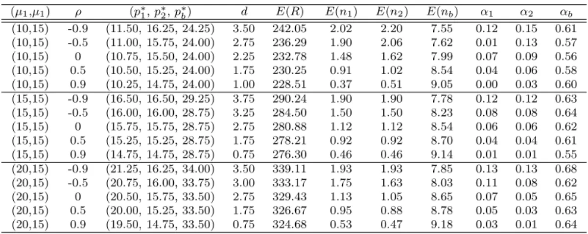
4.2 Optimization of p1, p2 and pb . . . 55
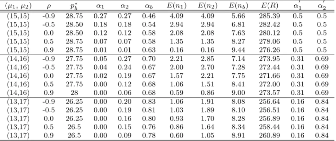
4.2.1 The Impact of Mean Reservation Prices . . . 57
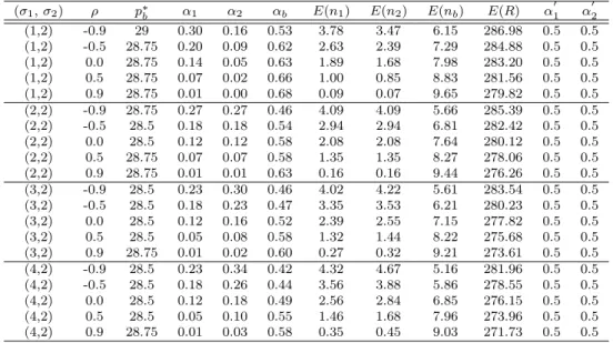
4.2.2 The Impact of Standard Deviation . . . 59
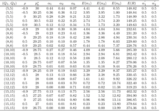
4.2.3 The Impact of Initial Inventory Levels . . . 59
4.2.4 The Impact of Customer Arrival Rate . . . 61
4.3 Other Strategies . . . 62
4.3.1 Pure Bundling . . . 62
4.3.2 Unbundled sales . . . 64
4.4 Comparison of the Bundling Strategies . . . 65
3.1 Purchasing Probabilities in Mixed Bundling Strategy . . . 28
3.2 No Stockout in both Products . . . 31
3.3 No Stockout in Product 1 and Stockout in Product 2 . . . 32
3.4 No Stockout in Product 2 and Stockout in Product 1 . . . 34
3.5 Product 1 is Depleted Before Product 2 . . . 36
3.6 Product 2 is Depleted Before Product 1 . . . 36
3.7 Both Products are Depleted Together . . . 37
4.1 Optimal Bundle Price when Individual Products are Fixed . . . . 47
4.2 Revenue vs. Bundle Price, p1=p2 . . . 49
A.1 Fixed p1 and p2: Equal individual product prices . . . 79
A.2 Fixed p1 and p2: Different individual product prices . . . 79
A.3 Fixed p1and p2: Different means for reservation price distributions,
p1=p2=15 . . . 80
A.4 Fixed p1 and p2: Means of reservation price distributions add up
to 30, p1=15, p2=15 . . . 80
A.5 Fixed p1 and p2: Different standard deviations for reservation price
distributions, p1=15, p2=15 . . . 81
A.6 Fixed p1 and p2: Equal standard deviations for reservation price
distributions, p1=15, p2=15 . . . 81
A.7 Fixed p1 and p2: Impact of starting inventory levels, p1=15, p2=15 82
A.8 Fixed p1 and p2: Impact of the arrival rate . . . 83
A.9 Optimization of p1, p2 and pb: Base case . . . 83
A.10 Optimization of p1, p2and pb: Different means for reservation price
distributions . . . 84 A.11 Optimization of p1, p2 and pb: Means of reservation price
distribu-tions add up to 30 . . . 84 x
A.12 Optimization of p1, p2 and pb: Different standard deviations for
reservation price distributions . . . 85
A.13 Optimization of p1, p2 and pb: Equal standard deviations for reser-vation price distributions . . . 85
A.14 Optimization of p1, p2 and pb: Different starting inventory levels . 86 A.15 Optimization of p1, p2 and pb: Equal starting inventory levels . . . 86
A.16 Optimization of p1, p2 and pb: Impact of the arrival rate . . . 87
A.17 Pure bundling: Base case . . . 87
A.18 Pure bundling: Impact of the arrival rate . . . 87
A.19 Pure bundling: Different means for reservation price distributions 88 A.20 Pure bundling: Means of reservation price distributions add up to 30 . . . 88
A.21 Pure bundling: Different standard deviations for reservation price distributions . . . 89
A.22 Pure bundling: Impact of starting inventory levels . . . 90
A.23 Unbundling: Base case . . . 90
A.24 Unbundling: Impact of the arrival rate . . . 91
A.25 Unbundling: Different means for reservation price distributions . . 91
A.26 Unbundling: Means of reservation price distributions add up to 30 92 A.27 Unbundling: Different standard deviations for reservation price distributions . . . 92
A.29 Comparison: Base cases . . . 93 A.30 Comparison: Percentage deviations for base cases . . . 94 A.31 Comparison: Different means for reservation price distributions . . 94 A.32 Comparison: Means of reservation price distributions add up to 30 95 A.33 Comparison: Different standard deviations for reservation price
distributions . . . 95 A.34 Comparison: Impact of the standard deviation . . . 96 A.35 Comparison: Impact of starting inventory levels . . . 96 A.36 Comparison: The impact of different starting inventory levels on
the performances of mixed and pure bundling . . . 97 A.37 Comparison: Impact of the arrival rate . . . 97
INTRODUCTION AND
DEFINITIONS
1.1
Introduction
Each organization involved in a production activity or providing services aims to do its best in terms of a performance criteria. Firms may have different objectives such as increasing their profits, their market shares, service levels or reducing operating costs. In order to achieve these goals, companies can follow different strategies. More efficient transportation, marketing and advertisement strategies, more profitable manufacturing methods may be employed to this end.
Most of the firms aim to maximize their profits by either increasing their rev-enues or cutting their costs down. Although all parties in a supply chain reduce their costs with improved inventory management, lost sales and excess invento-ries are still unavoidable. This is why, many companies are now looking into the demand side of the supply-demand relation. Retailers are the last party of supply chains. Most of the time, it is easier for retailers to improve profitability by efficient demand management instead of cost reduction. Better demand man-agement via efficient pricing policies becomes an important goal. Temporal price changes are becoming an industry practice to control revenue. However, the price
of the product cannot be increased or decreased arbitrarily. There should be some strategy that will dynamically adjust prices. Determining the strategy to use is a very complicated and difficult decision. Another way to achieve high revenues is to sell products to each customer at the best price that the customer is willing to pay, i.e., perfect price discrimination. However, it is almost impossible for a firm to know each individual’s valuation for products. Even if it is known, it will be unfair to charge each customer differently. Therefore, to improve revenues, a right price should be set for each product. Determining the right price to charge a customer for a product is a complex task. The company should know not only its supply and operating costs, but also how much the customers value the product and what the future demand will be. The retailer faces a trade-off when setting prices. If the retailer sets the prices too low, he will lose customers’ surplus; if he sets the prices too high he will lose the customer and risk having a surplus of goods at the end of the season.
Retail managers always face rapid changes in fashion and customer prefer-ences. Also, products may deteriorate with a rate depending on the age and/or amount of the products. Some items, on the other hand, may display negligible or no loss in quality and value during a fixed lifetime, after which they become useless or obsolete. Such products are called perishable. The ”perishability” of the products leads to short selling periods, during which inventory management and pricing strategies are central to success ([2]). Perishable inventories have re-ceived considerable attention in recent years. This is a realistic trend since most products such as medicine, dairy products and chemicals start to deteriorate once they are produced. Perishability also applies to services. The inventory of seats on a particular flight, the inventory of rooms at a hotel at a particular night all perish at certain times. Retailers and service providers have the opportunity to enhance their revenues through optimal pricing of their perishable products that must be sold within a fixed period of time. For fashion goods, the selling horizon is usually very short and production/delivery lead times prevent replenishment of inventory. Therefore, the seller has a fixed inventory on hand and must decide on how to price the product over remaining selling horizon.
of perishable products. The main idea behind revenue management is to divide the market into multiple customer classes and to provide different types of prod-ucts with different prices to each class. Success of yield management practices is closely related with advances in information technologies.
As stated before, determining the right price to charge is a complex task. There are different factors that influence the pricing decision of retailers. Some of these factors are reservation prices of customers, supply availability, intensity of customer arrivals, the length of the planning horizon, the behavior of the competitors and the prices of complementary and substitutable products. In the following paragraphs we explain how each factor affects pricing decisions. The findings provided below are supplemented from the following references: [6], [21] and [22].
Reservation price is defined as the maximum amount that the customer is willing to pay for a product. If the product’s price is lower than the reservation price of the customer, the customer buys the product, otherwise she does not. In marketing literature, ”value analysis” is used to explain how customers decide whether to buy the product or not by considering ”the perceived relative economic value” of the product. Accordingly, the maximum price that can be set is that at which customer disregards the difference between the product and the next best economic alternative. The difference between the maximum amount customers are willing to pay for the product and the amount they actually pay is called customers’ surplus (perceived acquisition value). This difference represents the customers’ gain from making the purchase (customers’ net gain from trade). It is usually assumed that the reservation price is a random variable with a continuous distribution over a population of customers and this distribution may change in time. The reasons for the variance in the reservation prices can be stated as the heterogeneity in the market (difference in income, age etc.) and a lack of information about the customer’s tastes and needs. The goal of the seller should be to adjust the prices so that the total expected profit is maximized over the planning horizon, while taking into consideration the heterogeneity of the population of customers in their willingness to pay for the product.
Almost all of the studies in the literature conclude that the profit increases with the level of the initial inventory. In some cases, the initial inventory is taken to be fixed due to some kind of commitments between the supplier and the retailer. The retailer should have an accurate forecasting strategy to determine the amount to order at the beginning of the planning horizon and an efficient strategy for pricing his initial inventory. Even in the case when the demand is not known in advance (and cannot be forecasted accurately) and the retailer has excess initial inventory, the prices should be set low (compared with valuation of customers) to increase the probability that all of the goods on hand will be sold. On the other hand, if the initial inventory is low and demand is known to be higher than the on hand inventory, the prices should be set high (again, compared with valuation of customers). In that case, the products will be sold to those customers with high reservation prices. Low prices with low initial inventory lead to the loss of the customer surplus. The retailer will then experience lost sales, loss of goodwill and decrease in market share since the inventory will be depleted before the horizon ends.
The arrival process of customers is another factor that affects the retailers’ pricing decisions. The arrival rate is often a response to their regular purchasing patterns during the selling season rather than a function of individual prices ([3]). The arrival pattern of the customers can be affected by advertisement campaigns. If the arrival intensity is dense, the prices are set high. Due to the high arrival rate, the probability of having customers with high reservation prices increases and high-price products are sold. However, when the arrival rate is small, it is more convenient to set the prices low. Otherwise, the small number of arriving customers will not purchase the product, resulting in increased holding cost, excess inventory on-hand and loss of the customer to the competitors.
Purchasing behavior of the customers also affects the retailer’s pricing deci-sions over time. Customers are divided as myopic and strategic according to their purchasing behavior. The first one makes a purchase immediately if the price is below his valuation, without considering future prices. The second type considers possible future prices of the product when making purchasing decision. There-fore, the seller should consider carefully the effects of his price over customers’
current and future decisions.
Another factor that affects the pricing decision of the seller is the length of the planning horizon. With short planning horizon, the initial price should be set low. Low prices will trigger the demand up and the possibility of selling all the units in this short period will increase. On the other hand, if we have a long planning horizon, we can set the initial price high. By setting the initial price high, we can get the customer surplus.
Pricing of a product in a competitive market is more difficult than in a mo-nopolistic one. In the absence of direct competition, one can estimate how a price change will affect sales simply by analyzing buyers’ price sensitivity. When, however, there is competition, the competitors can make sales estimates useless by changing their prices. In doing so, competitors change buyers’ alternatives and thus manipulate what they are willing to pay for it. For example, a com-pany might reasonably estimate that it could double sales by pricing 20 percent below the competitors. But a 20 percent price cut would not necessarily generate such a result. The competitors may respond with price cuts in their products to eliminate, narrow or even reverse the gain that the company hoped to achieve. The greater the potential for price competition, the more important it is for man-agement to evaluate how competitors are likely to use price in their marketing decisions.
Another factor that affects retailers’ pricing decisions is the prices of com-plementary and substitutable products. Most firms sell multiple products. For example, supermarkets sell products as diverse as meats, packaged goods, fur-niture, toys and clothing. If one product’s sales do not affect the sales of the firm’s other products, then it can be priced in isolation. Most often, however, the sales of the different products in the firm are interdependent. To maximize the profit, prices must reflect that interaction. The effect of one product’s sales on another’s can be either adverse or favorable. If adverse, then the products are ”substitutes”. Most substitutes are different brands in the same product class. Sometimes, however, substitutes appear in completely different product classes.
For example, the sales of macaroni products may rise whenever price increases re-duce the sales of beef. If one product’s sales favorably affect the sales of another, then the products are ”complements”. Complementarity can arise for either of two reasons: (1) the products are consumed together in producing satisfaction. For example, tickets to a movie and popcorn are complements; (2) the prod-ucts are most efficiently purchased together. Buyers often seek to conserve time and money by purchasing a set of products from a single seller. For example, consumers may get accustomed to a particular supermarket and buy all of their needs from there. Substitutes and complements call for adjustments in pricing when the products are sold by the same company as a part of a product line. To correctly evaluate the effect of a price change, management must examine the changes in revenues and costs not only for the product whose price is changed, but also for the other products affected by the price change.
In addition to the main characteristics discussed above, numerous other fac-tors can influence a dynamic pricing policy, such as business rules, cost of imple-menting price changes, seasonality of and external shocks to demand.
The common objective of almost all retailers is to maximize profits. There are different ways of achieving profit maximization. As explained in detail above, price adjustments are among the most useful ones. Another common strategy is to make promotions by selling two or more products in a bundle and charge a price less than the total amount that will be paid if products are bought individually. Bundling is a prevalent marketing strategy that takes considerable attention recently. Despite the increased interest on bundling, there are many questions that are left unanswered. For example, reasons for the profitability of bundling, conditions under which the retailers gain from bundling, customers perspective, legality of bundling are some of the subjects that seek further consideration.
Among many studies in the literature, Stremersch and Tellis [27] provides the clearest definitions of bundling terms and principles. They define bundling as the sale of two or more separate products in one package. Here, separate products refer to products for which separate markets exist. Seasonal tickets of sporting and cultural organizations, fixed-price menus, Internet services are
examples of bundling. Bundling can take one of two forms: price bundling or product bundling. In price bundling, the retailer sells two or more separate products in a package, without any physical integration of the products. Here bundling does not create added value to customers. Therefore, a discount must be offered to motivate at least some customers to buy the bundle. Selling tickets for different football matches at a price less than the sum of separate games’ ticket prices is an example for price bundling. On the other hand, product bundling is the integration and sale of two or more separate products or services at any price. A multimedia PC is an example for product bundling. The different functions of the individual parts are combined in a single product bundle. The multimedia PC has an integral architecture, in that it integrates functions such as connection, data storage, etc. By this integration, a complete PC can do more than the parts that are combined in can do. As a result, price bundling is a pricing and promotional tool, while product bundling is more strategic in that it creates added value. Price bundling is easier to implement compared with product bundling. The latter requires new design, new manufacturing plan, etc. All departments of a manufacturing company are involved in creation of product bundles. On the contrary, marketing departments are usually the only single decision makers for price bundling.
In order to clarify the concepts of price and product bundling, Stremersch and Tellis [27] give the following example: ”Consider strategic options of Dell, which markets to consumers who want to buy a portable computer system consisting of a basic laptop, a modem, and a CD burner. First, it can sell these products as separate items, such that the price of each item is independent of consumers’ purchase of the other item. In this case, consumers could easily give up purchasing a modem or CD burner, or they could purchase it from a competitor. Second, Dell can sell the products as a price bundle. For example, it could, without physically changing any of the products, give a discount to consumers if they buy all three products together. This offer would probably motivate at least some consumers to buy all three products from Dell. Third, Dell can sell the three items as a product bundle. To meet the latter classification, Dell must design some integration of the three separate products. For example, it could create an
enhanced laptop. Not only could this trigger some consumers to buy all products from Dell, but through the value added they might even do so at a premium price.”
Retailers most of the time use price bundling, which is the focus of this study. Therefore, from this point on, bundling refers to price bundling. This strategy can further be divided into two different types: pure and mixed. When retailers prefer pure bundling, they sell only the bundle but not the individual products. Mixed bundling is a strategy in which firm sells both the bundle and the separate products that constitute the bundle. Unbundling is a strategy in which products are sold separately, not as a bundle. Which strategy performs the best depends on many factors. Extensive literature concludes that there does not exist a single strategy that always dominates the other two.
The difficulty of making pricing decisions is mentioned above. Pricing becomes even more difficult when bundling is under consideration. Different customer seg-ments attach different values to each of the products that constitute the bundle. Some customers will want to purchase the bundle while others are interested in a specific product. Retailers should carefully decide on a pricing strategy for the individual products and for the bundle. Prices may encourage customers to select a wide range of offerings, including products that they do not value highly, or prices may encourage purchasing at increased prices. Each individual prod-uct as well as the bundle should be priced in a such a way that customers who value individual products highly are still willing to buy individual products and customers who do not want a component of the bundle become willing to buy a bundle.
In this study, pricing policy of a retailer selling two types of products is inves-tigated. He sells both the individual products and a bundle composed of them. Retailer’s aim is to maximize the revenue from the sales; cost of bundle forma-tion, cost of pricing software and other costs are ignored. Products are assumed to be perishable. There is a fixed planning horizon, during which replenishment is not possible. Therefore, the retailer has a fixed inventory of both products at the start of the season. He sets the prices at the beginning of the period and
these prices remains unchanged until the end of the period. The use of mixed bundling strategy is assumed, but the performances of other two strategies are investigated to form a benchmark for comparison.
1.2
Definitions
Reservation Price: The maximum amount that a customer is willing to pay
for a product.
Customer Surplus: The difference between the maximum amount customers
are willing to pay for the product and the amount they actually pay. This differ-ence represents the customers’ gain from making the purchase.
Complementary Products: If the sale of one product favorably affects the
sale of another product, these are called complementary products.
Substitutable Products: If the sale of one product adversely affects the sale of another product, these are called complementary products.
Myopic Customers: A customer who makes a purchase immediately if the
price is below her reservation price, without considering future prices.
Strategic Customers: A customer who takes into account the future path of
prices when making purchasing decision.
The rest of the thesis is organized as follows. In Chapter 2, an extensive literature review about pricing, bundling and bundle pricing is provided. In Chapter 3, the problem under consideration is defined, the model is introduced and possible realizations during the planning horizon are investigated. Depending on the numbers of individual products and bundles sold, the expected revenue function is obtained. Similar expressions are also obtained for pure bundling and unbundling cases. The performance of three strategies under different conditions, such as reservation price distribution of customers, the intensity of customer arrivals is explained via an intensive numerical study in Chapter 4. Finally, in
LITERATURE REVIEW
In literature, pricing problems have been studied extensively. There are a large number of research papers dealing separately with dynamic pricing or fixed num-ber of price changes of perishable products, timing and optimal duration of price changes, bundling of two or more products and pricing of bundles. Below, we present the literature about the theoretical background of these topics.
We will start with pricing of perishable products in the following section. Then, we will provide the literature on bundling, in which we will focus again on pricing studies. Finally, we will mention the shortcomings of the literature that motivated our study.
2.1
Pricing of Perishable Products
In recent years, pricing of perishable inventories has received considerable at-tention. Before providing a literature review about the pricing strategies for perishable products, we would like to emphasize the classification of general pric-ing strategies provided by Noble and Gruca [23]. Noble and Gruca divide the pricing strategies encountered in the industry into four broad categories: New Product Pricing Situation, Competitive Pricing Situation, Product Line Pricing
Situation and Cost-Based Pricing Situation. The conditions that determine when a given strategy should be used are referred to as determinants. Examples of de-terminants are product differentiation, economies of scale, capacity utilization, demand elasticity and product age.
New product pricing is appropriate in the early life of the product. This category has been divided into three strategies;
1. Price Skimming: In this strategy, the price is set high initially and then it is reduced over time gradually. The main objective is to attract customers who are insensitive to the initial high price. As this segment is saturated, the price is lowered to increase the appeal of the product.
2. Penetration Pricing: In this strategy, the price of the product is set low. The aim is to make customers accustomed to the product initially.
3. Experience Curve Pricing: In this strategy again the initial price is set low. However, the aim is to adopt the producer to this new product by building cumulative volume quickly and driving the unit cost down.
Competitive pricing is appropriate when the price of the product is deter-mined relative to the price of one or more competitors’ prices. This situation is categorized into three pricing strategies as follows;
1. Leader Pricing: The price leaders initiate price changes and they expect that others in the industry will follow their way in price adjustments. Generally, the price of an identical product is higher if it is sold by the leader company. 2. Parity Pricing: Firms that follow this strategy either tries to maintain a constant relative price between competitors or it imitates prevailing prices in the market.
3. Low Price Supplier: In this strategy, the firm sets the price lower than its competitors and it aims to have higher demand than the others.
Product line pricing situation corresponds to the situation where the price of the main product is affected by the other related products or services from the same company. There are three pricing strategies that are mentioned under this heading;
1. Complementary Product Pricing: The price of the main product is set low then the other complementary products. This strategy is well illustrated by Gillette’s strategy of selling razors cheaply and blades dearly.
2. Price Bundling: The product is offered as a component of a bundle of products. The total price of the bundle is set lower than the total price of the products bundled.
3. Customer Value Pricing: In this strategy one version of the product is offered at a very competitive price level, however the product involves fewer features than the other versions.
The fourth situation is cost-based pricing. The firm decides on how much to charge based on the cost incurred in obtaining the product.
This broad classification is valid for all kinds of products. Depending on the product type and on the market it is sold, a firm may need to use two or more of these strategies at the same time. This complicates the pricing decisions.
In the rest of this section, we will review the most frequently referred studies related with pricing of perishable products in the context of revenue management. One of the first studies related to dynamic pricing of perishable goods is by Rajan, Rakesh and Steinberg [24]. They investigate the relationship between pricing and ordering decisions for a monopolist retailer facing a known demand function where, over the inventory cycle, the product may exhibit physical decay or decrease in market value. The authors study the linear and nonlinear demand cases and exhibit propositions on the optimal price changes and optimal cycle length.
given stock of items that must be sold by a deadline. The demand is stochastic and price sensitive and the objective is revenue maximization. For exponential demand functions, the authors derive an optimal pricing policy in closed form. However, only the deterministic version of the problem is analyzed for general demand functions and an upper bound is obtained for the revenue. With this upper bound, the authors develop a single price policy, which is asymptotically optimal when either remaining shelflife or inventory volume is large. Gallego and van Ryzin [12] report that their policy provides a revenue that is only 5% to 12% below the optimal revenue when the number of items is fewer than 10 and it is nearly optimal for more than 20 items. This work is criticized by Feng and Xiao [11]. They suggest that for short remaining lives and small inventory volumes, the strategy of Gallego and van Ryzin would not work.
Yildirim, Gurler and Berk [34] consider the dynamic pricing of perishables in an inventory system where items have random lifetimes which follow a general distribution and the unit demands come from a Poisson Process with a price-dependent rate. The objective of their study is to determine the optimal pricing policy and the optimal initial stocking level to maximize the discounted expected profit. They consider the instances at which an item is withdrawn as a decision epoch for setting the sales price. Authors determine the optimal price paths for the discounted expected profit for various combinations of remaining lifetimes. Their study indicates that a single price policy results in significantly lower profits when compared with their formulation.
A dynamic pricing model for selling a given stock of a perishable product over a finite time horizon is considered by Zhao and Zheng [35]. They identify a sufficient condition under which the optimal price decreases over time for a given inventory level. They also illustrate that the optimal price decreases with inventory. According to their numerical analysis, their policy achieves 2.4-7.3% revenue improvement over the optimal single price policy.
Feng and Gallego [9] address the problem of deciding the optimal timing of a single price change from a given initial price to either a given lower or higher sec-ond price. It is shown that it is optimal to decrease (resp., to increase) the initial
price as soon as the time-to-go falls below (resp., above) a time threshold that de-pends on the number of yet unsold items. Later, the same authors study a similar problem [10]. They aim to decide again on the optimal timing of price changes within a given menu of allowable price paths each of which is associated with a general Poisson process with Markovian, time dependent, predictable intensities. Feng and Gallego [9] show that a set of variational inequalities characterizes the value functions and the optimal time changes. They develop an algorithm to compute the optimal value functions and the optimal pricing policy.
Bitran and Mondschein [3] study a problem similar to Gallego and van Ryzin [12] but the price is allowed to change only periodically. The price is never allowed to rise. Although, the authors present some empirical analysis for their study, no theoretical results are provided. Similarly, Chatwin [4] analyzes the pricing of perishable products where the set of available prices is finite. He indicates that for this problem as well as the problem in which the price is selected from an interval, the maximum expected revenue function is nondecreasing and concave in the remaining inventory and in the time-to-go. In addition, he shows that the optimal price is nondecreasing in the remaining inventory and nondecreasing in the time-to-go. He concludes that these results hold when prices and correspond-ing demand rates are functions of time-to-go but not when the demand rates are functions of inventory level.
There exist many studies in the literature that reveals the fact that the pric-ing decisions must be given in coordination with other managerial decisions. The overall objective of the firm can only be achieved by considering all the impor-tant decisions at once. Federgruen and Heching [8]’s address the simultaneous determination of pricing and inventory replenishment strategies under demand uncertainty. They show that a base stock list price policy is optimal for the finite horizon with bi-directional price changes. In a base stock list price policy; if the inventory level is below the base stock level, it is raised to the base stock level and the list price is charged. If inventory level is above the base stock level, then nothing is ordered and price discount is offered. Similarly, Wee and Law [33] develop a replenishment and pricing policy by taking into account the time value of money. The inventory system under consideration is deterministic and
demand is price-dependent. They derive a near optimal heuristic to maximize the total net present-value profit. Subrahmanyan and Shoemaker [30] study a pric-ing model that allows replenishments and incorporates learnpric-ing about demand through Bayesian updates. The model they use is a dynamic programming model which is solved numerically using backward recursion.
Chun [5] also considers the problem of determining the price for several units of a perishable or seasonal product to be sold over a limited period of time. He assumes that the customer’s demand can be represented as a negative binomial distribution and determines the optimal product price based on the demand rate, buyers’ preferences and the length of the sales period. Since the seller’s average revenue decreases as the number of items for sale increases, Chun [5] also considers the optimal-order-quantity that maximizes the seller’s expected profit. He also develops a multi-period pricing model, for the cases where the seller can divide the sales period into several short periods.
Bitran, Caldentey and Mondschein [2] examine the coordination of clearance markdown sales of seasonal products in retailer chains. The authors propose a methodology to set prices of perishable items in the context of a retail chain with coordinated prices among its stores and compare its performance with actual practice in a case study. A stochastic dynamic programming problem is formu-lated and heuristic solutions that approximate optimal solutions satisfactorily are developed.
Elmaghraby and Keskinocak [7] provide a review of the literature and current practices in dynamic pricing. Their focus is on dynamic (intertemporal) pricing in the presence of inventory considerations. This paper constitutes a good summary for dynamic pricing policies.
In this section we reviewed a limited number of papers related with pricing of perishable products.
2.2
Bundle Pricing
Bundling is a prevalent marketing strategy. Despite its importance, little is known about how to find optimal bundle prices and only a few studies are available in the literature. In this section, we will review the most influential studies about bundling and bundle pricing.
Most of the bundling papers are built on the early study of Stigler [28],where the author represents the demand information by reservation prices for the prod-ucts. Additivity of reservation prices and production costs is assumed. He con-cludes that bundling is profitable when reservation prices are negatively corre-lated.
Adams and Yellen [1] develop a two-product, monopoly bundling model by assuming that the reservation prices for products are additive and negatively cor-related. They show that the profitability of commodity bundling can stem from its ability to sort customers into groups with different reservation price charac-teristics, extracting consumer surplus. They consider a monopolist producing two goods with constant unit costs and facing buyers with diverse tastes. The authors assume a discrete number of customers. The reservation prices for the components of the bundle are negatively correlated. This feature makes it appear that bundling serves much the same purpose as third-degree price discrimination. Authors consider three different sales strategies: unbundling, pure bundling and mixed bundling and compare these strategies in terms of seller profit. Adams and Yellen [1] argue that mixed bundling at least weakly dominates pure bundling. The reason is that, customers with negatively correlated reservation prices prefer individual products, while the others prefer the bundle. The low bundle valuation of the demanders make mixed bundling a more profitable strategy compared to pure bundling. The authors’ argument presume that bundling does not lead to any cost savings.
Schmalensee [26] also developes a two-product monopoly bundling model in which he relaxes the assumption that the reservation prices of the individual prod-ucts are negatively correlated. However, he retained the additivity assumption.
By assuming that reservation prices (for firm’s two products) are distributed ac-cording to bivariate normal probability law, Schmanlensee constructs a class of examples within which the profitability of bundling can be analyzed as a func-tion of producfunc-tion costs, the mean and variance of the reservafunc-tion price for each commodity, and the correlation between the two commodities’ reservation prices. The author obtains some general results for mixed bundling case and compares them with pure bundling and unbundled sales. After comparing pure bundling with unbundled sales, Schmalensee [26] shows explicitly that pure bundling oper-ates by reducing the effective dispersion in buyers’ tastes. This happens simply because as long as reservation prices are not perfectly correlated, the standard deviation of reservation prices for the bundle is less than the sum of the standard deviations for the two components. The greater is the average willingness to pay, measured as the normalized difference between mean reservation price and cost, the more likely it is that such a reduction in diversity will enhance profits by per-mitting more efficient capture of consumers’ surplus. If the average willingness to pay is large enough, the increase in profit caused by pure bundling is apparently larger than the fall in consumers’ surplus, so that pure bundling increases net welfare. Besides, Schmalensee [26] provides a comparison of the profitability of mixed bundling and unbundled sales. It is shown that mixed bundling combines the advantages of pure bundling and unbundling sales. This policy enables the seller to reduce effective heterogeneity among those buyers with high reservation prices for both goods, while still selling at a high markup to those buyers willing to pay a high price for only one of the goods. At least in the Guassian case, this makes mixed bundling a very powerful price discrimination device. One of the surprising findings of this paper is that bundling can be profitable when de-mands are uncorrelated or even positively correlated. To summarize, two major results of his work are a confirmation of the profitability of bundling when there is negative correlation, and the benefits of mixed bundling over a restriction to unbundling or pure bundling. Two comments are written to this paper by Long [18] and Jeuland [17].
Long [18] states that heterogeneity in consumer tastes (especially in rela-tive valuations of the firm’s two products) is a necessary condition for profitable
bundling. Unfortunately, more specific principles to describe concisely the nec-essary and/or sufficient conditions for profitable bundling are not so obvious. Different from Schmalensee [26], the author assumes that the distribution of con-sumer reservation prices has a continuous density without restricting it to any particular form. He states that, if an increase in prices (above the monopoly level) increases the number of consumers who buy only one of the two commodities, the bundling will increase profit. Besides, if the reservation prices for the two commodities are not positively correlated, then bundling increases profit. When bundling does not increase profit, a form of promotional couponing does increase the profit. Long [18] concludes that the most favorable case for bundling as a price discrimination device is the case where the bundle components are substitutes in demand.
Jeuland [17] also comments on the paper of Schmalensee [26]. The author states that, depending on the distribution of reservation price, any ranking- in terms of profitability for the seller- of these three strategies is possible.
Salinger [25] focuses on the graphical analysis of bundling and he deals with two-product case. He assumes additive reservation prices. Salinger explores the implications of the relationship between the bundle and aggregated components demand curves for the profitability and welfare effects of bundling. If it does not lower costs, bundling tends to be profitable when reservation values are negatively correlated and high relative to costs. If bundling lowers costs and costs are high relative to reservation values, positively correlated reservation values increase the incentive to bundle.
None of these papers show how to calculate optimal bundle prices. One impor-tant study that draw attention to this topic is the study of Hanson and Martin [14] in which they provide a practical method for calculating optimal bundle prices. The basis of the approach is to formulate the model as a mixed integer linear program using disjunctive programming. The theoretical rationale for this ap-proach is given along with computational results for a set of test problems based on actual survey data. An added benefit of the bundle pricing model solution is stated to be the selection of products to include in a firm’s product line. Authors
also consider one of the most serious problems facing a product line manager addressing the bundling issue: the exponential growth in possible products which results from increasing the number of components considered. An algorithm for finding optimal solutions is given along with computational results.
The published studies are fuzzy about some basic terms and principles, do not discuss the legality of bundling, and do not provide a comprehensive framework on the economic optimality of bundling. Stremersch and Tellis [29] provide a new synthesis of the field of bundling based on a critical review and extension of the marketing, economics and law literature. This paper clearly and consis-tently defines bundling terms and principles. Authors identify two key underly-ing dimensions of bundlunderly-ing that enable a comprehensive classification of bundlunderly-ing strategies and formulate clear rules to evaluate the legality of each strategy. In addition, authors propose a framework of twelve propositions that prescribe the optimal bundling strategy in various contexts. The propositions incorporate all the important factors that influence bundling optimality.
As reviewed before, bundling has received considerable attention in economics and marketing literature. Most research in this area studies the conditions un-der which bundling is profitable for the seller and/or the customer. The general result is that the profitability of bundling depends on the distribution of reser-vation prices. The previous research also compares the performance of different strategies such as mixed bundling, pure bundling and unbundling and concludes that no unique strategy dominates the others in all circumstances.
We note that bundling studies in economics and marketing literature make an implicit assumption that there is an ample supply of products that could be acquired at a certain cost. In this thesis, however, we assume that there is a fixed amount of inventory for each product to be sold over a finite horizon, and we study how individual and bundle products should be priced to maximize revenue from this limited inventory. In this respect, our study follows the line of yield management or revenue management research. We should also note that while the existing research in marketing and economics literature study the performance of different bundling strategies, they do not consider optimizing the bundle and
the individual product prices explicitly. In this thesis, our focus is on optimizing the bundle price individually or bundle and individual prices jointly. We assess the performance of different bundling strategies given that pricing decisions are optimally taken.
MODEL and THE ANALYSIS
Based on the studies related with bundle pricing in literature, it is observed that very few researchers consider the determination of prices that maximize the revenue in mixed bundling strategy. In this study, we focus on the expected revenue maximization for the mixed bundling strategy with two products and stochastic demand. Given an initial inventory of two products and a finite selling season, we are concerned with the problem of determining prices of the bundle and the individual products so that the expected revenue over the selling season is maximized. To form a basis of comparison, we also study pure bundling and unbundling strategies.
Before defining the problem under consideration, we elaborate on some of the fundamental assumptions used in our model. We first note that we use reservation prices to predict purchasing behavior of customers arriving to the store. Consumer reservation price is a fundamental concept in understanding consumer purchasing decisions and developing pricing strategies. We refer the reader to Jedidi and Zhang [16] for estimating individual consumer reservation prices and to Jedidi et. al [15] for capturing consumer heterogeneity in the joint distribution of reservation prices in the case of bundling. Other ways to model consumer behavior in the case of differentiated products include multinomial logit (MNL) random utility model; see van Ryzin and Mahajan [31] and Mahajan and van Ryzin [19].
We assume that the reservation price for the bundle is equal to the sum of the individual reservation prices. This reflects the assumption that the products are individually valued. Many of the bundling studies in literature (e.g., Adams and Yellen [1], Schmalensee [26], McAfee [20]) use the same assumption. Guiltinan [13] refers to this assumption as the assumption of strict additivity. Venkatesh and Kamakura [32] relax the strict additivity assumption and allow for substi-tutability and complementarity. If the products are substitutable, customers want to buy only one of them at a time. Then, a customer’s reservation price for the bundle would be subadditive (less than the sum of the reservation prices). Alternatively, customers may tend to consume the two products together. These kind of products are called complementary. When products are complements, a customer’s reservation price for the bundle is superadditive (more than the sum of the reservation prices).
We also assume that customers’ reservation price pairs follow a bivariate nor-mal distribution. According to Schnor-malensee [26], the frequency with which nornor-mal distributions arise in the social sciences makes the Gaussian family a plausible choice to describe the distribution of tastes in a population of buyers. The bivari-ate normal has a small number of easily interpreted parameters. Because the sum of two normal distributions is also normal, the distributions of reservation prices for the bundle and the components have the same form, when strict additivity is assumed. In addition, handling correlations between demands for the components is simple when normal distributions are used. A problem with normal is that it entails negative valuations. Salinger [25] states that, while there may be cases where customers would pay not to receive a good, the assumption of negative valuations is not appropriate whenever an undesirable component of a bundle can be disposed of freely. Therefore, we select appropriate parameters for the normal distributions in our numerical study to ensure non-negative valuations.
3.1
Problem Definition
We consider a retailer who sells two perishable products, Product 1 and Product 2. Initially, Q1 units of Product 1 and Q2 units of Product 2 are available. There
is a fixed planning horizon of length T over which the sales are allowed and the retailer aims to maximize his profit.
It is assumed that the retailer forms a monopoly for the two products. At the beginning of the planning horizon, the retailer sets the price p1 for
Product 1, and p2 for Product 2. He also provides a bundle option which implies
charging the customers less than the sum of the individual products’ prices if they buy both. The individual product prices and the bundle price, pb are determined
so that pb ≤ p1 + p2. We assume that the initial prices remain unchanged until
the end of the season. It is assumed that, the retailer incurs fixed costs before the selling season. We therefore consider maximizing the revenue.
Customers arrive at the store according to a Poisson Process with a fixed arrival rate of λ customers/period. A customer is allowed to purchase a single product or a bundle, not both. She may also choose to leave without any purchase. Customers’ preferences are reflected by their reservation prices. The reservation price is defined as the maximum amount that a customer is willing to pay to purchase a product. If the product prices are lower than the reservation prices, she prefers the product which brings her maximum surplus (the reservation price for the product - the price of the product).
Customers’ reservation prices are assumed to be random variables with con-tinuous distributions. Specifically, we assume that the reservation prices for the two products, referred to as R1 and R2, respectively are normally distributed
with parameters (µ1, σ1) and (µ1, σ1), respectively. The reservation price for the
bundle is assumed to be the sum of the individual products’ reservation prices, i.e., Rb = R1 + R2. Therefore, we assume products are independent. We define
the correlation coefficient of the joint reservation price distribution as ρ.
products and the bundle with their corresponding prices. She decides to leave without any purchase, buy Product 1, Product 2 or a bundle, with probabilities, α0, α1, α2 and αb, respectively. In calculation of these probabilities, it is assumed
that at least one unit exists from each product. If at any point during the planning horizon, one of the products is depleted, these probabilities change. Let, α10 be the probability of buying Product 1, after depletion of Product 2. Similarly, α0
2 is
defined as the probability that a customer buys Product 2 when Product 1 is not available. A customer may leave without a purchase with probability α0
01=1-α
0
1
, when Product 2 is depleted and with probability α0
02=1-α
0
2, when Product 1 is
depleted. Note that no bundle can be purchased when either of Product 1 or Product 2 is depleted.
We assume that the retailer knows the reservation price distributions and that he follows a mixed bundling strategy.
In the following sections we derive expressions to calculate the expected rev-enue for a given set of bundle and individual product prices. Then, these expres-sions are used to find the bundle and individual product prices that will maximize the expected revenue.
3.2
Problem Formulation
3.2.1
Preliminaries
Before deriving the purchasing probabilities,we introduce some preliminary con-cepts. Let R1 and R2 denote the reservation prices of the two products and
fR1,R2(r1, r2) denote their joint probability density function, with corresponding marginals fR1(x) and fR2(x). Assuming bivariate normal distribution for the joint probability, we have fR1,R2(r1, r2) = e−θ(r1,r2)/2 2πσ1σ2p1 − ρ2 , , where θ(r1, r2) = 1 1 − ρ2[( r1− µ1 σ1 )2− 2ρ(r1− µ1 σ1 )(r2− µ2 σ2 ) + (r1− µ1 σ1 )2].
where ρ is the correlation between the reservation prices. Then, for i = 1, 2 we have the following marginal distributions for the reservation prices Ri, with mean
µi and standard deviation σi:
fRi(r) =
e−(r−µi)2/2σ2i σi
√ 2π
Under bivariate normality, it is straightforward to show that the distribution of reservation price, Rb=R1+R2 for the bundle (consisting of one unit of each good)
is normal with mean µb = µ1+ µ2. The standard deviation of Rb is calculated as:
σb = (σ1+ σ2)δ,
where δ = [1 − 2(1 − ρ)θ(1 − θ)]1/2, and θ = σ1/(σ1+ σ2).
3.2.2
Purchasing Probabilities
3.2.2.1 Purchasing probabilities when there is no stockout
Suppose first that both products are available at the store so that the customer buys either a single product, or a bundle or leaves without any purchase. The probabilities of these events are given below:
Probability of No Purchase:
A customer will purchase nothing when her reservation prices for the indi-vidual products and the bundle are lower then their corresponding sales prices. Thus the probability of no purchase is given by,
α0 = P (R1 < p1, R2 < p2, Rb < pb) = P (R1 < p1, R2 < p2, R1+ R2 < pb) = P (R1 < p1, R2 < min {p2, pb− R1}) = Z p1 −∞ Z a1 −∞ fR1,R2(r1, r2)dr1dr2 where a1=min{p2, pb− r1}.
Probability of Purchasing Product 1:
A customer will purchase Product 1 if her surplus (the difference between the reservation price and sales price) is positive and larger than her surplus from Product 2 and the bundle. Thus the probability of purchasing Product 1 is given by, α1 = P (R1 > p1, R1 − p1 > R2− p2, R1− p1 > Rb − pb) = P (R1 > p1, R1 − p1 > R2− p2, R1− p1 > R1+ R2 − pb) = P (R1 > p1, R2 < min {R1− p1+ p2, pb− p1}) = Z ∞ p1 Z a2 −∞ fR1,R2(r1, r2)dr1dr2 where a2=min {r1 − p1+ p2, pb− p1} .
Probability of Purchasing Product 2:
A customer will purchase Product 2 if her surplus is positive and larger than her surplus from Product 1 and the bundle. Thus the probability of purchasing Product 2 is given by,
α2 = P (R2 > p2, R2 − p2 > R1− p1, R2− p2 > Rb − pb) = P (R2 > p2, R2 − p2 > R1− p1, R2− p2 > R1+ R2 − pb) = P (R2 > p2, R1 < min {R2− p2+ p1, pb− p2}) = Z ∞ p2 Z a3 −∞ fR1,R2(r1, r2)dr2dr1 where a3=min {r2 − p2+ p1, pb− p2} .
Probability of Purchasing a Bundle:
A customer will purchase the bundle if her surplus is positive and larger than the surplus from Product 1 and Product 2. Thus the probability of the bundle purchase is given by,
Product 2 Product 1 Bundle r1 r2 p1 p2 pb pb pb-p2 pb-p1 No purchase
Figure 3.1: Purchasing Probabilities in Mixed Bundling Strategy
αb = P (Rb > pb, Rb− pb > R1− p1, Rb− pb > R2− p2) = P (Rb > pb, R1+ R2− p2 > R1− p1, R1+ R2− pb > R2− p2) = P (R1 > pb − p2, R2 > max {pb− R1, pb− p1}) = Z ∞ pb−p2 Z ∞ a4 fR1,R2(r1, r2)dr1dr2 where a4=max {pb− r1, pb− p1}
Purchasing probabilities are depicted in Figure 3.1.
3.2.2.2 Probabilities when there is a stockout
The above probabilities are valid when both products are available. At any point during the planning horizon one of the products can be depleted. Then, an ar-riving customer can no longer purchase the bundle. She can either buy one unit from the remaining product or leave the store buying nothing. The probabilities for these cases are found as follows.
Product 1 is depleted before Product 2
Suppose that Product 1 has been depleted. An arriving customer either pur-chases Product 2 or leave the store without a purchase. If customer’s reservation price for Product 2 is less than its price, she buys nothing. The probability for this case is given by,
α002 = P (R2 < p2)
= Z p2
−∞
fR2(r2)dr2.
If customer’s reservation price for Product 2 is larger than its price, she buys Product 2. The probability for this case is given by,
α02 = P (R2 > p2) = Z ∞ p2 fR2(r2)dr2 = 1 − α002.
Product 2 is depleted before Product 1:
Suppose that Product 2 has been depleted. An arriving customer either pur-chases Product 1 or leave the store without a purchase. If customer’s reservation price for Product 1 is less than its price, she buys nothing. The probability for this case is given by,
α001 = P (R1 < p1)
= Z p1
−∞
fR1(r1)dr1.
If customer’s reservation price for Product 1 is larger than its price, she buys Product 1. The probability for this case is given by,
α01 = P (R1 > p1) = Z ∞ p1 fR1(r1)dr1 = 1 − α001
It has already been stated that customers arrive to the store according to a Poisson Process with an arrival rate of λ customers/period. When both products
are available, sales of Product 1 (Product 2, bundle) follows a Poisson Process with the sale rate of λα1 (λα2, λαb) products/period. Similarly, when Product 1
(Product 2) is depleted the sales of Product 2 (Product 1) sold follows Poisson Process with rate of λα02 (λα01) products/period.
Having calculated the purchasing probabilities, in the following section, we derive expressions to calculate the probabilities for different sale realizations dur-ing the planndur-ing horizon. Before proceeddur-ing with that, note that by assumdur-ing p1+ p2 > pb, we justify our assumption that in the mixed bundling case the
cus-tomer buys either Product 1 or Product 2 or bundle since she does not prefer to buy Product 1 and Product 2 together for a price equal to or larger than p1+ p2.
3.3
Sales Probabilities and the Objective
Func-tion
3.3.1
Sales Probabilities for Different Realizations
In order to find the expected revenue at the end of the planning horizon, we need to know how many units of Product 1, Product 2 and bundle are sold. Let N1, N2 and Nb be the number of Product 1, Product 2 and the bundle that are
sold during the planning horizon and let
P (n1, n2, nb) = P (N1 = n1, N2 = n2, Nb = nb)
be the joint probability function for the sales, where the period starts with Q1 of
Product 1 and Q2 of Product 2.
Before we write the the objective function we first derive the expressions for P (n1, n2, nb) for different realizations. The derivation of the joint probability
function, P (n1, n2, nb), needs some careful consideration. Clearly, there are four
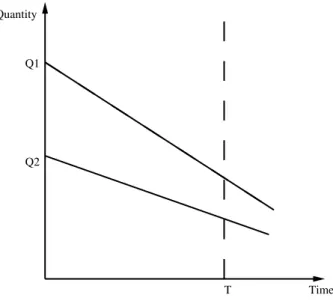
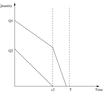
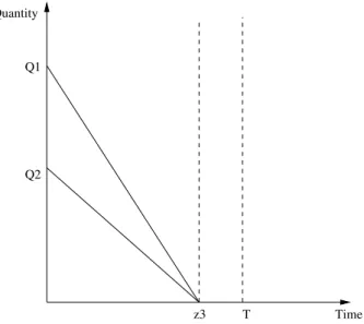
possible structures for the period realizations: 1) No stockout in any products (Figure 3.2), 2) Stockout only in Product 2 (Figure 3.3), 3) Stockout only in Product 1 (Figure 3.4), and 4) Stockout in both products (Figure 3.5, Figure 3.6
Time Quantity
Q1
Q2
T
Figure 3.2: No Stockout in both Products
and Figure 3.7). When there is stockout in both products, one should also keep track of the order of the stockout times since the order changes the dynamics of the purchasing behavior of the customers.
Next, the calculation of P (n1, n2, nb) for each of the above cases is illustrated.
3.3.1.1 Case 1: No stockout in both products
No stockout occurs during the planning horizon. Hence, we have both Product 1 and Product 2 left. That is;
N1+ Nb < Q1
N2+ Nb < Q2.
The probability of a particular realization N1 = n1, N2 = n2, Nb = nb in this
case can be calculated as,
P (n1, n2, nb) = P n1 Product 1 purchases in [0, T ] n2 Product 2 purchases in [0, T ] nb bundle purchases in [0, T ]
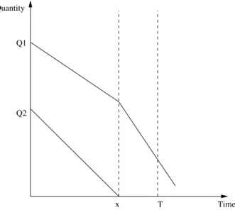
Time Quantity Q1 Q2 T x
Figure 3.3: No Stockout in Product 1 and Stockout in Product 2
P (n1, n2, nb) = e−λα1T(λα 1T )n1 n1! e−λα2T(λα 2T )n2 n2! e−λαbT(λα bT )nb nb!
The first (second, third) expression is the probability that n1 (n2, nb) units of
Product 1 (Product 2, bundle) is sold in the interval [0,T ].
Case 2: No Stockout in Product 1 and Stockout in Product 2 Product 2 is depleted during the planning horizon but at the end, there is at least one unit of Product 1 on hand. That is;
N1+ Nb < Q1
N2+ Nb = Q2.
In order to calculate the probability of a particular realization, N1 = n1, N2 = n2,
Nb = nb, we need to condition on the time at which the inventory of Product
2 is depleted. Let x be this time and let N11(x) be the number of Product 1
that is sold in the interval [0, x]. The last purchase that depletes the inventory of Product 2 can be either an individual purchase of Product 2 or a bundle purchase. If the last purchase is an individual purchase, nth
2 individual purchase of Product
2 is realized at time x and there are nb bundle purchases in the interval [0, x).
If the last purchase is a bundle purchase, then nth
b bundle purchase is realized at
either case, if N11(x) = n11, there are n11Product 1 purchases in the interval [0, x]
and n1− n11 Product 1 purchases in the interval (x, T ]. Thus, for this stockout
situation, the probability of a particular realization n1, n2, nb can be expressed
as: P (n1, n2, nb) = I(n2 ≥ 1) Z T 0 n1 X n11=0 P n11 Product 1 purchases in [0, x] n1− n11 Product 1 purchases in (x, T ] nb bundle purchases in [0, x) fn2,α2λ(x) dx + I(nb ≥ 1) Z T 0 n1 X n11=0 P n11 Product 1 purchases in [0, x] n1 − n11 Product 1 purchases in (x, T ] n2 Product 2 purchases in [0, x) fnb,αbλ(x) dx
where fn2,α2λ is the density of an Erlang n2 random variable with rate α2λ and fnb,αbλ is the density of an Erlang nb random variable with rate αbλ. Thus, we have P (n1, n2, nb) = I(n2≥1) ZT 0 n1 X n11=0 e−λα1x(λα 1x)n11 n11! e−λα0 1(T −x)(λα0 1(T − x))n1 −n11 (n1−n11)! e−λαbx(λα bx)nb nb! fn2,α2λ(x)dx + I(nb≥1) ZT 0 n1 X n11=0 e−λα1x(λα1x)n11 n11! e−λα0 1(T −x)(λα0 1(T − x))n1 −n11 (n1−n11)! e−λα2x(λα2x)n2 n2! fnb,αbλ(x)dx where fn2,α2λ(x) = (λα2)n2xn2−1e−λα2x (n2− 1)! fnb,αbλ(x) = (λαb)nbxnb−1e−λαbx (nb− 1)! .
In the above expression, the first integral corresponds to the probability of a particular realization n1, n2, nb where the last purchase that depletes the inventory
of Product 2 is an individual purchase. In order for this to happen, we should have at least one individual Product 2 sold. This is why an indicator function appears before the integral and it equals to 1 if we have at least one Product 2 purchase. The sum inside the integral is over all possible realizations of number of individual Product 1 sold up to x. Note that the time of the nth
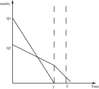
Time Quantity Q1 Q2 T y
Figure 3.4: No Stockout in Product 2 and Stockout in Product 1
purchase is an n2 Erlang random variable, since it corresponds to the waiting
time until the nth
2 Poisson event with rate of α2λ.
The second integral corresponds to the probability of a realization where the last purchase that depletes the inventory of Product 2 is a bundle purchase. Note that we need to have at least one bundle purchase for this case to happen. Ww have I(nb ≥ 1)=1, if the number of bundles sold is greater than one. On the
other hand, if nb=0, we have I(nb ≥ 1)=0 and the second integral is not added
to the sale probability.
Case 3: No Stockout in Product 2 and Stockout in Product 1 Product 1 is depleted during the planning horizon but at the end, there is at least one unit of Product 2 on hand. That is;
N1+ Nb = Q1
N2+ Nb < Q2.
Similar to the previous case, let y be the time at which inventory of Product 1 is depleted and N21(y) be the number of Product 2 that is sold in the interval
[0,y]. The last purchase that depletes the inventory of Product 1 can be either an individual purchase of Product 1 or a bundle purchase. If the first event happens,