C om mun.Fac.Sci.U niv.A nk.Series A 1 Volum e 66, N umb er 2, Pages 349–361 (2017) D O I: 10.1501/C om mua1_ 0000000825 ISSN 1303–5991
http://com munications.science.ankara.edu.tr/index.php?series= A 1
NUMERICAL SOLUTIONS OF THE MRLW EQUATION USING MOVING LEAST SQUARE COLLOCATION METHOD
AY¸SE GÜL KAPLAN AND YILMAZ DEREL·I
Abstract. In this paper, the Modi…ed Regularized Long Wave (MRLW) equation is solved by using moving least square collocation (MLSC) method. To show the accuracy of the used method several numerical test examples are given. The motion of single solitary waves, the interaction of two soli-tary waves and the Maxwellian initial condition problems are chosen as test problems. For the single solitary wave motion whose analytical solution is known L2, L1error norms are calculated. Also mass, energy and momentum
invariants are calculated for every test problem. Obtained numerical results are compared with some earlier works. According to the obtained results, the method is very e¢ cient and reliable.
1. Introduction
The regularized long wave (RLW) equation was de…ned for the …rst time by Peregrine [1] to introduce the behavior of the bore development. Later Benjamin et al. used as model for a larger class of physical phenomena. The modi…ed regularized long wave equation (MRLW) is a special form of RLW equation. This equation plays a very important role at the modelling of the nonlinear, dispersive media being modeled feature small-amplitude, long-wave length disturbances. The MRLW equation has the following form
Ut+ Ux+ "U2Ux Uxxt= 0 (1)
where " and are positive integers and subscripts x and t denote space and time derivatives, respectively.
The exact solution of the MRLW equation was found by as follows [3] U (x; t) =
r 6c
" sech (k (x (c + 1)t x0]) (2) Received by the editors: July. 29, 2016; Accepted: February 03, 2017.
2010 Mathematics Subject Classi…cation. 65M70 .
Key words and phrases. Moving least square collocation method, MRLW equation.
c 2 0 1 7 A n ka ra U n ive rsity C o m m u n ic a tio n s d e la Fa c u lté d e s S c ie n c e s d e l’U n ive rs ité d ’A n ka ra . S é rie s A 1 . M a th e m a t ic s a n d S t a tis t ic s .
where k =q (c+1)c , x0 and c are arbitrary constants. For the single solitary wave
6c=" is the amplitude of solitary wave and its width is represented by k, also x0 is
the peak position of the wave. This solitary wave propagates to the right side by keeping its original shape at a steady velocity c + 1 while time is increasing, [14]. In this study numerical experiments will be performed for the parameter " = 6, = 1, c = 1 and x0 = 40. In the present study, in order to …nd a numerical solution
of the MRLW equation on the …nite domain [a; b], boundary conditions and initial condition are chosen as follow, respectively:
U (a; t) = 0; U (b; t) = 0; a x b; t > 0
U (x; 0) = f (x): (3)
The MRLW equation has been solved numerically by using numerical techniques. These include …nite element, …nite di¤erence, Fourier method and meshless meth-ods. The MRLW equation was solved by various types of B-spline functions by using …nite element method such as the collocation method with quintic B-splines …nite element method in [3], the collocation method using cubic B-splines …nite element in [7], a numerical scheme based on quartic B-spline method in [17], based on collocation of quintic B-splines …nite elements in [18] was presented. Also the collocation method with quadratic, cubic, quartic and quintic B-splines [10], cubic B-spline lumped Galerkin …nite element method [11], a Petrov-Galerkin method [13] were used.
A …nite di¤erence scheme and Fourier stability analysis in [5], two …nite di¤er-ence approximations for the space dicretization and a multi-time step method for the time discretization for the MRLW equation in [15] and a fully implicit …nite di¤erence method in [19] were presented for the numerical solution of the MRLW equation. Also, the Adomian decomposition method was applied to solve numeri-cally the MRLW equation in [6].
The meshless methods were applied to the MRLW equation in the literature. The meshless kernel based method of lines was used in [8] where gaussian, multi-quadric and Wendland’s compactly supported radial basis functions were used as kernel functions in computations. The radial basis functions collocation method by using di¤erent shape functions which were multiquadric, gaussian, inverse mul-tiquadric and inversequadric radial basis functions was applied in [9]. A meshless method based on the moving least-squares approximation for the nonlinear gener-alized regularized long wave equation was used in [16]. In where the cubic spline function was used as weight function also convergence of the iterative process was presented.
In this study, the moving least square collocation method by using gaussian weight function will be applied to the MRLW equation and obtained results will be com-pared with other results in the literature.
2. The moving least square approximation
To solve the MRLW equation (1) numerically, the moving least square collocation (MLSC) approximation will be applied. Lancaster and Salkauskas [12] de…ned a local approximation for u(x) as follow
uh(x)=
m
X
i=1
pi(x)ai(x) = pT(x)a(x) (4)
where pi(x) is the given monomial basis function of order m, ai(x) are the
un-known coe¢ cients of basis functions at spatial coordinates x. uh(x) represents the
MLS approximation of u(x). The unknown coe¢ cients ai(x) will be determined by
minimizing the weighted discrete error norm given by
J (x) = N X i=1 !(x xi)[uh(x) u(xi)]2 = N X i=1 !(x xi) 2 4 m X j=0 pj(x)aj(x) u(xi) 3 5 2
where !(x xi) are weight functions, xi are nodes of spatial coordinates x: To …nd
the value of vector a(x) by minimizing the J we obtain @J
@a = A(x)a(x) B(x)u = 0 so this can be written in the equation system
A(x)a(x) = B(x)u, from this resulting equation a(x) is found as
a(x) = A 1(x)B(x)u
where the matrices A(x), B(x), u, W(x) and p(x) are de…ned as follow: A(x) = pT(x)W(x)p(x);
B(x) = pT(x)W(x); uT = (u1; u2; :::; uN);
W(x) = 2 6 6 6 4 !(x x1) 0 0 0 !(x x2) 0 .. . ... . .. ... 0 0 !(x xN) 3 7 7 7 5; p(x) = 2 6 6 6 4 p0(x1) p1(x1) pm(x1) p0(x2) p1(x2) pm(x2) .. . ... . .. ... p0(xN) p1(xN) pm(xN) 3 7 7 7 5:
Therefore, substituting a(x) into Eq. (4) approximation function of u(x) is obtained as
u(x) uh(x) = pT(x)A 1(x)B(x)u or u(x) uh(x) = N X i=1 i(x)ui= T(x)u: (5)
T(x) is a matrix of shape function and has the following form
(x) = ( 1(x); 2(x); :::; N(x)) (6)
= pT(x)A 1(x)B(x) where i(x) has the following form
i(x) = m
X
j=0
pj(x) (A 1(x)B(x)) ji: (7)
In the literature there are some weight functions and in our algorithms Gaussian weight function with compact supported is chosen. Gaussian weight function is de…ned as follows !(x xi) = 8 > < > : e (di=ci)2 e (ri=ci)2 1 e (ri=ci)2 ; 0 di ri 0; di> ri (8)
where ciis the shape parameter and di= jx xij is the distance between collocation
points x and xi. The support size rifor weight functions !(x xi) determines the
support of node xi. Derivatives of the approximate solution uh(x) can be obtained
as @k @xku h(x) = n X i=1 @k i(x) @xk ui: (9)
3. Discretization of the MRLW equation
In this section, the MRLW equation is discretized by using a Crank-Nicolson scheme for U and a forward di¤erence rule for Utin time as following:
Un+1 Un t + Un+1 x + Uxn 2 + 6 U2U x n+1 + U2U x n 2 Un+1 xx Uxxn t = 0: (10)
Eq. (10) can be rewritten as Un+1 Un+ t 2 U n+1 x + Uxn +3 t U2Ux n+1 + U2Ux n Uxxn+1 Uxxn = 0: (11) The nonlinear term (U2U
x)n+1in Eq. (11) may be linearized by using Taylor series
expansion as follows U2Ux
n+1
= (U2)nUxn+1+ 2UnUxnUn+1 2 U2 nUxn: (12) Substituting Eq. (12) in to the Eq. (11) time-discretized the MRLW equation can be written as Un+1+ t 2 U n+1 x Uxxn+1+ 3 t (U2)nUxn+1+ 2UnUxnUn+1 = Un t 2 U n x Uxxn + 3 t U2)nUxn : (13)
4. Implementation of the MLSC method
In this section, the MLSC method will be applied to the discretized form of the MRLW equation (13). To …nd the numerical value of U used approximation is given as follows Un = N X i=1 i(xk) ni; k = 1; 2; ; N (14)
where i(xk) are shape functions at each collocation points xk and i are the
unknown values. Eq. (14) can be written as the following matrix form
Un= ~A n (15) where ~ A = [ i(xk) : i; k = 1; N ]; n= [ n1; n 2; ; n N]T:
First and second derivatives of Eq. (14) given by Uxn= N X i=1 0 i(xk) ni; Uxxn = N X i=1 00 i(xk) ni; k = 1; 2; ; N (16)
respectively. We put our trial functions Eqs. (14) and (16) into the Eq. (13) and Eq. (3) at the collocation points xk; gives the following systems of algebraic
equations: N P i=1 i (xk) n+1i + t 2 N P i=1 0 i(xk) n+1i + 3 t N P i=1 2 i(xk) ni N P i=1 0 i(xk) n+1i +6 t N P i=1 i (xk) ni N P i=1 0 i(xk) ni N P i=1 i (xk) n+1i N P i=1 00 i(xk) n+1i = N P i=1 i (xk) ni t 2 N P i=1 0 i(xk) ni + 3 t N P i=1 2 i(xk) ni N P i=1 0 i(xk) ni N P i=1 00 i(xk) ni; k = 2; : : : ; N 1 N P i=1 i (xk) n+1i = ; k = 1 N P i=1 i (xk) n+1i = ; k = N (17)
Substituting Eq. (7) into Eq. (17) and simplifying we have obtain following linear equation system
M1 n+1= ; k = 1 5 P j=1 Mj n+1= 3 P j=1 Mj n M4 n ; k = 2; : : : ; N 1 M1 n+1= ; k = N (18)
where coe¢ cients Mj are de…ned as follows:
M1= N P i=1 m P j=0 pj(xk)[A 1(xk)B(xk)]ji M2= N P i=1 m P j=0 pj(xk)[A 1(xk)B(xk)] 00 ji M3= 3 t N P i=1 m P j=0 pj(xk)[A 1(xk)B(xk)]2ji n i N P i=1 m P j=0 pj(xk)[A 1(xk)B(xk)] 0 ji M4= 6 t N P i=1 m P j=0 pj(xk)[A 1(xk)B(xk)]ji ni N P i=1 m P j=0 pj(xk)[A 1(xk)B(xk)] 0 ji ni N P i=1 m P j=0 pj(xk)[A 1(xk)B(xk)]ji M5= N P i=1 m P j=0 pj(xk)[A 1(xk)B(xk)] 0 ji
By solving the equations system (18) numerical values of n+1are obtained at each nodal points. Substituting these values into the Eq. (14) numerical values of the MRLW equation at the each nodal points on solution interval is obtained.
5. Numerical examples and comparisons
In this section, MRLW equation are solved for three test problems to demonstrate accuracy and e¢ ciency of the method. Also, conserved quantities and error norms will be calculated for test problems.
The MRLW equation has three conservation laws which are [4] C1= b Z a U dx; C2= b Z a U2+ (Ux)2 dx; C3= b Z a (U4 (Ux)2)dx
and corresponding to conservation of mass, momentum and energy respectively. In our computations numerical values of invariants are computed by using rectangular rule.
The root mean square error L2 and maximum error L1will be used to measure
the error between the analytical and numerical solutions: L2= s h N P j=1 Uexact j Ujnum: 2 ; L1= max 1 j N U exact j Ujnum: :
5.1. Test 1: Single solitary wave motion. The single solitary wave solution of the MRLW equation is written as follow:
U (x; t) =pc sech (k [x (c + 1)t x0]) ; k =
r c (c + 1)
For numerical calculations, boundary conditions U (0; t) = U (100; t) = 0 and initial condition U (x; 0) = pc sech (k [x x0]) are used. Simulations are done over the
solution domain 0 x 100 in the time period 0 t 10 with parameters h = 0:2; t = 0:025, = 1, c = 1 and x0= 40. The analytical values of invariants
are given as [3] C1 = p c k = 4:44288 C2 = 2c k + 2 kc 3 = 3:29983 (19) C3 = 4c2 3k 2 kc 3 = 1:41421
At the time t = 10, calculated values of invariants C1, C2, C3 and error norms
L2, L1 are listed in Table 1. It is clear that, obtained results are all in very good
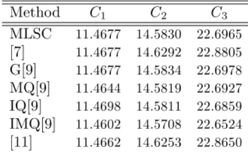
wave pro…le is depicted in Figure 1 at di¤erent times. From Figure 1, it is seen that solitary wave propagates to the right along the x-axis without changing its shape.
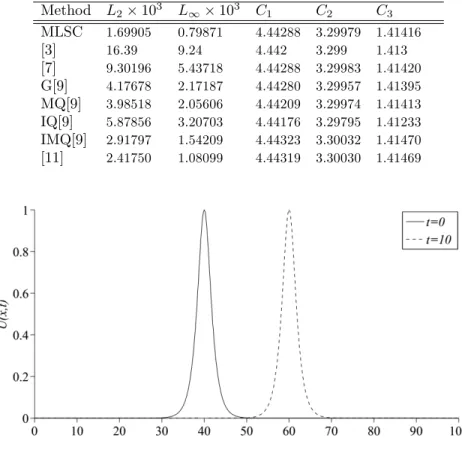
Table 1 : Comparison of invariants and error norms.
Method L2 103 L1 103 C1 C2 C3 MLSC 1.69905 0.79871 4.44288 3.29979 1.41416 [3] 16.39 9.24 4.442 3.299 1.413 [7] 9.30196 5.43718 4.44288 3.29983 1.41420 G[9] 4.17678 2.17187 4.44280 3.29957 1.41395 MQ[9] 3.98518 2.05606 4.44209 3.29974 1.41413 IQ[9] 5.87856 3.20703 4.44176 3.29795 1.41233 IMQ[9] 2.91797 1.54209 4.44323 3.30032 1.41470 [11] 2.41750 1.08099 4.44319 3.30030 1.41469
Figure 1. Motion of the single solitary wave.
5.2. Test 2: Interaction of Two Solitary Waves. Interaction of two positive solitary waves for MRLW equation is modelled by using the following initial condi-tions U (x; 0) = 2 X j=1 pc j sech (ki(x xj)) ; kj= r cj (cj+ 1) (19) where xj, cj are arbitrary constants, j = 1; 2. In this test problems, parameters are
chosen = 1, c1 = 4, c2 = 1, x1 = 25, x2 = 55 over the solution domain [0; 250]
analytical values of invariants are given as [3] C1= 2 P j=1 pc j kj = 11:4677; C2= 2 P j=1 (2cj kj + 2 kjcj 3 ) = 14:6292; C3= 2 P j=1 (4c 2 j 3kj 2 kjcj 3 ) = 22:8805: (20)
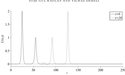
Calculated values of invariants are tabulated in Table 2. Obtained results are compared with analytical and other numerical results [7, 9, 11]. Two solitary waves pro…les are depicted in Figure 2 and 3 at di¤erent times. As seen from these …gures, the larger wave moves faster than the smaller one and it catches up and passes the smaller wave as time progresses. It is seen from …gures a small tail occurs after completed of interaction of waves because these waves are solitary waves not solitons. It is known that solitary waves don’t obey the principle of superposition. When the faster wave overtakes a slower wave, again solitary waves don’t combine and add together [15].
Table 2: Comparison of invariants.
Method C1 C2 C3 MLSC 11.4677 14.5830 22.6965 [7] 11.4677 14.6292 22.8805 G[9] 11.4677 14.5834 22.6978 MQ[9] 11.4644 14.5819 22.6927 IQ[9] 11.4698 14.5811 22.6859 IMQ[9] 11.4602 14.5708 22.6524 [11] 11.4662 14.6253 22.8650
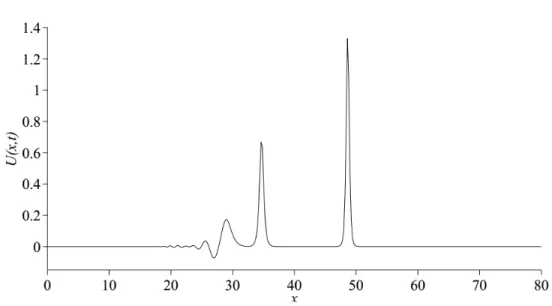
5.3. Test 3: The Maxwellian initial condition. Maxwellian initial condition for MRLW equation is de…ned as
U (x; 0) = exp( (x x0)2):
Boundary conditions are taken as U (0; t) = U (80; t) = 0 in the time period 0 t 10. The computed values of the invariants for = 0:1, = 0:05, = 0:025, x0 = 20, h = 0:2 and 4t = 0:01 are recorded in Table 3. Obtained results are
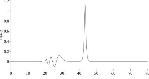
compared with numerical results in [13]. It is seen that from Figures 4, 5 and 6 the number of solitary wave is increased when is reduced. For instance, a single solitary wave is occurred in Figure 4 while a few solitary wave is occurred in Figure 5 and 6.
Figure 2. Interaction of two solitary waves at di¤erent times.
Figure 3. Interaction of two solitary waves at t = 10.
Table 3: Computed values of invariants.
Method C1 C2 C3 MLSC 0.1 1.77245 1.38255 0.75714 [13] 0.1 1.77245 1.3808 0.7618 MLSC 0.05 1.77245 1.32353 0.82520 [13] 0.05 1.77246 1.31898 0.825787 MLSC 0.025 1.77245 1.27829 0.894994 [13] 0.025 1.77245 1.28935 0.863683 Figure 4. Maxwellian initial condition at t = 10 for = 0:1.
Figure 4. Maxwellian initial condition at t = 10 for = 0:1.
Figure 6. Maxwellian initial condition at t = 10 for = 0:025.
6. Conclusion
The MRLW equation is solved numerically by using moving least square collo-cation method. The performance of the used numerical method with the di¤erent three test problems which are the single solitary wave motion, interaction of two solitary waves and the Maxwellian initial condition have been examined. The error norms L2 and L1 for the single solitary wave motion have been calculated. Also,
for the examined test problems numerical values of three conserved quantities have been evaluated. It has been seen that evaluated numerical results are in good agree-ment with the results obtained by previous studies. According to obtained results, the method satis…ed very highly acceptable results for the MRLW equation. This method is a meshless method hence has the simplicity of implementation and very high accuracy. The obtained results indicate that the present method is very e¤ective and reliable numerical technique for solving this type nonlinear equations. It should point that the used numerical technique can be applied to nonlinear prob-lems.
References
[1] D.H. Peregrine, Calculations of the development of an undular bore, J. Fluid Mech., 25(1966), 321-330.
[2] T.B. Benjamin, J.L. Bona and J.J. Mahony, Model equations for waves in nonlinear dispersive systems, Phil. Trans. Roy. Soc. London A, 227(1972), 47-78.
[3] L.R.T. Gardner, G.A. Gardner, F.A. Ayoub and N.K. Amein, Approximations of solitary waves of the MRLW equation by B-spline …nite elements, Arab. J. Sci. Eng., 22(1997), 183-193.
[4] P.J. Olver, Euler operators and conservation laws of the BBM equation, Math. Proc. Camb. Philos. Soc., 85(1979), 143-159.
[5] A.K. Khalifa, K.R. Raslan and H.M. Alzubaidi, A …nite di¤erence scheme for the MRLW and solitary wave interactions, Appl. Math. Comput., 189(2007), 346-354.
[6] A.K. Khalifa, K.R. Raslan and H.M. Alzubaidi, Numerical study using ADM for the modi…ed regularized long wave equation, Appl. Math. Model., 32(2008), 2962-2972.
[7] A.K. Khalifa, K.R. Raslan and H.M. Alzubaidi, A collocation method with cubic B-splines for solving the MRLW equation, J. Comput. Appl. Math., 212(2008), 406-418.
[8] Y. Dereli, Numerical solutions of the MRLW Equation Using Meshless Kernel Based Method of Lines, International Journal of Nonlinear Science, 13(2012), 28-38.
[9] Y. Dereli, Solitary wave solutions of the MRLW Equation Using Radial Basis Functions, Numerical Methods in Partial Di¤erential Equations, 28(2012), 235-247.
[10] K.R. Raslan and S.M. Hassan, Solitary Waves for the MRLW equation, Applied Mathematics Letters, 22(2009), 984-989.
[11] S.B.G. Karakoç, Y. Uçar and N.M. Ya¼gmurlu, Numerical solutions of the MRLW equation by cubic B-spline Galerkin …nite element method, Kuwait J. Sci., 42(2015), 141-159. [12] P. Lancaster and K. Salkauskas, Surfaces generated by moving least square methods,
Math-ematics of Computation, 87(1981), 141-158.
[13] T. Roshan, A Petrov-Galerkin method for solving the generalized regularized long wave (GRLW) equation, Computers and Mathematics with Applications, 63(2012), 943-956. [14] ·I. Da¼g, D. Irk, and M. Sar¬, The extended cubic B-spline algorithm for a modi…ed regularized
long wave equation, Chin. Phys. B, 22(2013), 040207.
[15] P. Keskin and D. Irk, Numerical solution of the MRLW equation using …nite di¤erence method, International Journal of Nonlinear Science, 14(2012), 355-361.
[16] W. Ju-Feng, B. Fu-Nong, and C. Yu-Min, A meshless method for the nonlinear generalized regularized long wave equation, Chinese Physics B, 20(2011), 030206.
[17] F. Haq, S. Islam, and I.A. Tirmizi, A numerical technique for solution of the MRLW equation using quartic B-splines, Applied Mathematical Modelling, 34(2010), 4151-4160.
[18] S.B.G. Karakoç, N.M. Ya¼gmurlu, and Y. Uçar, Numerical approximation to a solution of the modi…ed regularized long wave equation using quintic B-splines, Bundary Value Problems, 27(2013), 1-17.
[19] B. ·Inan, A.R. Bahad¬r, Numerical Solutions of MRLW Equation by a Fully Implicit Finite-Di¤erence Scheme, Journal of Mathematics and Computer Science, 15(2015), 228-239.
Current address : Ay¸se Gül Kaplan: Osmaniye Korkut Ata University, Mathematics Depart-ment, 80000, Osmaniye, Turkey
Current address : Y¬lmaz Dereli: Anadolu University, Mathematics Department, 26470, Es-ki¸sehir, Turkey