İSTANBUL BİLGİ UNIVERSITY INSTITUTE OF SOCIAL SCIENCES
FINANCIAL ECONOMICS MASTER’S DEGREE PROGRAM
OPTIMALITY ANALYSIS of FINANCIAL DERIVATIVE PRODUCTS in TURKISH MARKET
Cem Eminoğlu
116620027
Associate Professor Serda Selin Öztürk
İSTANBUL 2019
iii
FOREWORD
I would like to thank my wife Kübra Eminoğlu due to her patience, support and intellection on my thesis process.
iv TABLE OF CONTENTS FOREWORD ... İİİ ABBREVIATIONS ... Vİİİ LIST OF FIGURES ...İX LIST OF TABLES ...X ABSTRACT ...Xİ ÖZET ...Xİİ INTRODUCTION ... 1 LITERATURE SURVEY ... 3 METHODOLOGY ... 5 SECTION ONE ... 6
1. EXCHANGE TRADED MARKETS AND ITS HISTORICAL DEVELOPMENT ... 6
1.1. ANCIENT TIMES ... 6
1.2. MIDDLE AGES ... 6
1.3. RENAISSANCE ... 7
1.4. INDUSTRIAL REVOLUTION AND AFTER ... 7
1.5. ELECTRONIC MARKETS... 9
SECTION TWO ... 9
2. OVER THE COUNTER MARKETS ... 9
2.1. GENERAL INFORMATION ABOUT OTC MARKETS ... 9
2.2. MARKET SIZE ... 10
SECTION THREE ... 11
3. INSTRUMENTS OF RISK HEDGING ... 11
3.1. FORWARDS ... 11
3.1.1. FORWARD CONTRACTS ... 11
3.1.2. PAYOFFS FROM FORWARD CONTRACTS ... 13
3.1.3. GENERAL FEATURES OF FORWARD CONTRACTS ... 14
3.2. FUTURES ... 14
3.2.1. FUTURES CONTRACTS ... 14
3.2.2. GENERAL FEATURES OF FUTURES CONTRACTS ... 15
3.2.3. STANDARD ELEMENTS OF FUTURES CONTRACTS... 16
3.3. OPTIONS ... 17
3.3.1. OPTION CONTRACTS ... 17
v
3.3.3. BASIC ELEMENTS THAT DETERMINE OPTION PRICES ... 20
3.3.4. MAIN TWO DIFFERENCES OF OPTIONS FROM FORWARD-FUTURES: ... 21
3.4. COMPARISON OF FORWARD-FUTURES-OPTION ... 21
3.5. TYPES OF TRADERS WHICH MAKE TRANSACTIONS ON DERIVATIVE MARKET ... 22
3.5.1. HEDGERS ... 22
3.5.2. SPECULATORS ... 23
3.5.3. ARBITRAGEURS ... 25
3.6. SWAPS ... 25
3.6.1. INTEREST RATE SWAPS ... 26
3.6.1.1. FIXED-VARIABLE INTEREST RATE SWAPS ... 26
3.6.1.2. VARIABLE-VARIABLE INTEREST RATE SWAPS ... 26
3.6.1.3. FIXED-FIXED INTEREST RATE SWAPS ... 27
3.6.2. CURRENCY SWAPS ... 27
3.6.3. COMMODITY SWAPS ... 27
3.7. NEW GENERATION DERIVATIVES ... 28
3.7.1. WARRANTS ... 28
3.7.1.1. STOCK WARRANTS ... 28
3.7.2. EXOTIC OPTIONS ... 28
3.7.2.1. TYPES OF EXOTIC OPTIONS ... 29
3.7.3. FUTURES OPTIONS ... 29
SECTION FOUR ... 30
4. FINANCIAL DERIVATIVE PRICING MODELS ... 30
4.1. FORWARD PRICING MODEL ... 30
4.2. FUTURES PRICING MODELS ... 31
4.2.1. COST OF CARRY MODEL... 31
4.2.2. STOCK INDICES MODEL ... 33
4.3. OPTION PRICING MODELS ... 34
4.3.1. BLACK AND SCHOLES MODEL ... 34
4.3.2. ADDITION TO OPTION PRICING-FACTORS THAT AFFECT THE OPTION PREMIUM ... 36
4.3.2.1. REMAINING TIME TO MATURITY ... 37
4.3.2.2. VOLATILITY RATIO ... 38
4.3.2.3. RISK-FREE RATE ... 39
4.3.2.4. DIVIDEND ... 39
4.3.2.5. DELTA ... 40
vi 4.3.2.7. VEGA ... 41 4.3.2.8. THETA ... 41 4.3.2.9. RHO ... 41 4.3.3. BLACK MODEL ... 41 4.3.4. ROLL-GESKE-WHALEY MODEL ... 41 4.3.5. BJERKSUND-STENSLAND 2002 MODEL ... 42 4.3.6. GARMAN-KOHLHAGEN MODEL ... 42
4.4. SWAP PRICING MODELS ... 42
4.5. WARRANT PRICING MODELS ... 42
SECTION FIVE ... 43
5. DERIVATIVE MARKETS IN TURKEY ... 43
5.1. OTC MARKET ... 43
5.2. EXCHANGE TRADED MARKETS ... 45
5.3. ORGANIZATION STRUCTURE OF EXCHANGE TRADED MARKETS AND PARTIES ... 46
5.3.1. STOCK MARKET ... 47
5.3.2. CLEARING HOUSE ... 48
5.3.3. INTERMEDIARY INSTITUTIONS (MEMBERS) ... 48
5.3.4. SUPERVISORY INSTITUTIONS ... 49
SECTION SIX ... 49
6. BORSA İSTANBUL A.Ş (BİST) ... 49
6.1. MARKETS ... 49
6.1.1. MECHANISM OF VİOP ... 50
6.1.1.1. INSTRUMENTS TRADING IN VİOP ... 50
6.1.1.2. ACCOUNT TYPES OF VİOP ... 50
6.1.1.3. TRANSACTION HOURS OF VİOP ... 50
6.1.1.4. SIZE OF CONTRACT ... 51
6.1.1.5. PRICE TRICK ... 51
6.1.1.6. LAST TRANSACTION DAY ... 51
6.1.1.7. ORDER METHODS ... 51
6.1.1.8. CONTRACT CODES ... 52
6.1.1.9. UNDERLYING ASSETS ... 52
6.1.2. PRICING APPLICATIONS IN VİOP AND ITS OPTIMALITY ... 53
6.1.2.1. FUTURES PRICING APPLICATION IN VİOP ... 53
6.1.2.2. OPTION PRICING APPLICATION IN VİOP ... 53
vii
REFERENCES ... 67
APPENDIX ... 69
APPENDIX 1: DETAILED AND UPDATED INFORMATION ABOUT THE SIZE OF OTC DERIVATIVE MARKET ... 69
APPENDIX 2: DETAILED AND UPDATED INFORMATION ABOUT THE SIZE OF EXCHANGE TRADED DERIVATIVE MARKET ... 72
APPENDIX 3: TYPES OF UNDERLYING ASSETS AT VİOP ... 73
APPENDIX 4: CALL EQUITY OPTIONS TEST RESULTS ... 76
APPENDIX 5: CALL INDEX OPTIONS TEST RESULTS ... 78
APPENDIX 6: CALL CURRENCY OPTIONS TEST RESULTS ... 79
APPENDIX 7: PUT EQUITY OPTIONS TEST RESULTS ... 81
APPENDIX 8: PUT INDEX OPTIONS TEST RESULTS ... 82
APPENDIX 9: PUT CURRENCY OPTIONS TEST RESULTS ... 83
APPENDIX 10: MATLAB CODES FOR MODELS ... 84
viii
ABBREVIATIONS
CBOT: Chicago Board of Trade
CBOE: Chicago Board Options Exchange
CME: Chicago Mercantile Exchange
BIST: Borsa Istanbul
DTB : German Exchange Traded Market
SOFEX: Switzerland Stock
VIOP: Derivative Market of Turkey
OTC: Over-the-Counter
GDP: Gross Domestic Product
CAPM: Capital Asset Pricing Model
ix
LIST of FIGURES
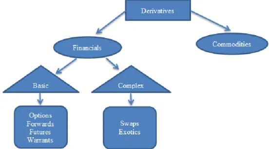
Figure 1: Classification of derivative products according to Gupta (2017) ... 1
Figure 2:Payoffs from forward contracts; (a) long position, (b) short position. Delivery price=K; price of asset at contract maturity=ST ... 13
Figure 3: Net profit per share from (a) purchasing a contract consisting of 100 Google December call options with a strike price of $520 and (b) selling a contract consisting of 100 Google September put options with a strike of $480. ... 20
Figure 4: Value of Microsoft holding in 2 months with hedging and without hedging. ... 23
Figure 5: Profit or loss from two alternative strategies for speculating on a stock currently worth $20 ... 24
Figure 6: Time Value of Option Graph ... 37
Figure 7: Implied Volatility Rate ... 39
Figure 8: Foreign Exchange and Gold Contracts OTC Market (in millions of USD) ... 44
Figure 9: Equity, Commodity, Credit and "Other" Derivatives OTC Market (in millions of USD) ... 44
Figure 10: Volume of Options, Futures and Their Total Values ... 45
Figure 11: Role of Clearing House at the Delivery Process ... 48
Figure 12: Underlying Asset Sample from Excel ... 54
Figure 13: Annual Compound Base Interest Rate Per Day... 55
Figure 14: MATLAB Output Example for Black and Scholes Model ... 56
Figure 15: MATLAB Output Example for Garman-Kohlhagen Model ... 56
Figure 16: MATLAB Output Example for Roll-Geske-Whaley Model ... 57
Figure 17: MATLAB Output Example for Bjersund-Stensland 2002 Model ... 58
Figure 18: Call Equity Option Test Output from Excel ... 59
Figure 19: Call Index Option Test Output from Excel ... 60
Figure 20: Call Currency Option Test Output from Excel ... 61
Figure 21: Put Equity Option Test Output from Excel ... 62
Figure 22: Put Index Option Test Output from Excel ... 63
x
LIST OF TABLES
Table 1: Size and Market Value of OTC markets ... 10
Table 2: Forward and spot quotes for the GBP/USD exchange rate, May 24, 2010 (GBP=British pound; USD= US dollar; quote is number of USD per GBP) ... 12
Table 3: Prices of Call Options on Google, June 15, 2010; stock price: bid $497.07; offer $497.25 (Source: CBOE) ... 18
Table 4: Prices of Put Options on Google, June 15, 2010; stock price: bid $497.07; offer $497.25 (Source: CBOE) ... 19
Table 5: The Effect of Basic Elements That Determines Option Prices to Option Premium ... 20
Table 6: Comparison of Forward-Futures-Option ... 21
Table 7: Comparison of profits from two alternative strategies for using $2000 to speculate on a stock worth $20 in October. ... 24
Table 8:Transaction Hours ... 50
Table 9: Options Contracts ... 52
xi
ABSTRACT
Optimality Analysis of Financial Derivative Products in Turkish Market
Financial derivative applications are purchased from abroad by Turkish institutions. However, critical point is whether these programmes are optimal in Turkish market.
Firstly, common types of derivatives and their applications are going to be stated in global market. After that different financial derivative applications are going to be considered and analyzed. In conclusion, optimality test of financial derivatives in Turkish market is going to be conducted at Matlab progmamme.
Keywords: Derivatives, Financial Derivatives, OTC and Exchange Traded
xii
ÖZET
Türkiye Piyasasında Finansal Türev Ürünlere İlişkin Uygulamaların Optimalite Analizi
Türkiye’de finansal türev uygulamaları bankalar tarafından yurtdışından hazır olarak alınmaktadır. Buradaki en kritik nokta hazır alınan program uygulamalarının Türk finansal türev piyasası için optimal olup olmadığıdır.
Öncelikle dünyadaki genel türevler ve farklı finansal türevler uygulamalarından bahsedilecek ve sonra dünyadaki farklı finansal türev uygulamaları araştırılıp, analiz edilecektir. Daha sonra Türk piyasasındaki finansal türev uygulamaları farklı senaryolarla Matlab programında kod yazılarak optimalite testi yapılacaktır.
Anahtar Kelimeler: Türev Ürünler, Finansal Türevler, Organize Olan ve
1
INTRODUCTION
There had been an intensive globalization wave in the world from beginnings of 1990’s to 2016, when Trump was elected in the United States and Britain decided to leave the European Union. International commerce and business volume had increased rapidly in this period. Consequently, demand for money had surged and some financial instruments had rallied. Financial risks had gone up due to changes in prices of stock markets and exchange rates. Financial engineering instruments or financial derivatives were come to exist to mitigate increased financial risks.
There are four types of financial derivatives; forward at over the counter markets, futures at exchange traded markets, options and swaps at both of markets. Furthermore, derivatives are not only financial products, there are many non-financial derivatives such as cotton, wheat, corn, soy bean, oil, natural gas, gold, silver, copper, nickel and so on.
2
When fund managers, financial institutions and treasury managers trading at over the counter markets evaluate investment opportunities or issue bonds/bills, they benefit many types of financial and non-financial derivatives.
Hull (2012) states “you could like of hate derivatives, but you cannot ignore them”.
The stock market is much smaller than derivative market according to comparison of value of their underlying assets. Moreover, value of derivative market is much bigger than world Gross Domestic Product (GDP). However, derivative products were criticized as one of vital reasons for mortgage crisis in US, 2007, because derivative products were formed with using risky mortgages as underlying asset in that period. Value of derivative products was decreased because of fall in house prices and it caused a big problem. Today, regulations on derivative products have bolstered.
Exchange traded and over the counter markets and their historical developments and size is going to be stated in next chapters. Financial derivative products are also going to be analyzed at this thesis project.
3
LITERATURE SURVEY
Black and Scholes (1971) option valuation model was tested by estimation of equity variances. Black and Scholes (1973) it was stated that theoretical and market prices of options are different, also option buyers buy at higher costs according to theoretical prices. Sterk (1983) it was considered that dividend payment is ignored at Black and Scholes European type option pricing model, although it is reckoned at Roll-Geske-Whaley option pricing model. Riskmetrics-Technical Document (1996) it was demonstrated that decay factor for EWMA model is 0.94. Galati and Tsatsaronis (1996) it was stated that neither implied nor historical volatility is better in long term while implied volatility is better in short term for anticipation periods of instability to predict volatility of underlying assets of currency options. Derosa (1998) Garman-Kohlhagen Option Pricing Model was stated. Chen (1998) implied volatility in foreign currency options was stated. Bjerksund and Stensland (2002) pricing model of American call and put options was explained. Zumbach (2006) it was considered that decay factor for exponential weighted moving average is 0.94 according to widen empirical studies. Qin and Li (2008) European call and put options were formulized at uncertain financial markets. Also, some pricing models were stated by coding with Matlab program. Suleimenov (2009) it was stated that theoretical and Turkish market prices may be different by using Binomial and Black and Scholes models. Jacque (2010) history of derivatives and malpractices of financial derivatives were demonstrated. Jabbour and Budwick (2010) financial derivatives and strategies regarding them were considered. Jaresova (2010) EWMA style estimators were compared with GARCH estimators and it was stated that EWMA style estimators were better. Chenchen (2011) Monte Carlo simulation model for call options and Binomial model for put option were used to explain differences between theoretical and market prices. Akmehmet (2012) six sub models were created with changing volatility and interest rates and their theoretical prices were compared by using Black and Scholes model. Bennet (2012) different measures of historical
4
volatility were stated and briefed. Akyapı (2014) it was stated that usage of Black-Scholes-Merton option pricing model is not efficient at Turkish derivative market. SPL Registry and Training Notes (2018) historical development and main differences of derivatives such as forward, futures and options were stated. Moreover, option pricing with Black and Scholes model was stated.
5
METHODOLOGY
There are 3 main types of options contracts, which are single stock, equity index and currency contracts, traded in Borsa İstanbul Futures and Options Market. Furthermore, single stock options have 30, index options have 3 and currency options have 6 types of underlying equities. The underlying asset prices for the related options and Turkey one month swap, USA one month swap and indicator interest rate data will be provided from the Bloomberg terminal.
Firstly, daily returns of listed underlying assets of options will be calculated. After that their daily variances and standard deviations will be reckoned. Then, annual volatility, which equals to daily standard deviation product by square root of 252 days, will be estimated by using of daily standard deviations. Later, estimated and enabled data will be run by Matlab application. Consequently, theoretical prices with regard to Black and Scholes, Roll-Geske-Whaley, Garman-Kohlhagen and Bjersund and Stensland models will be measured. In conclusion, it will be determined and interpreted whether there is difference between theoretical and market prices.
6
SECTION ONE
1. EXCHANGE TRADED MARKETS AND ITS HISTORICAL DEVELOPMENT
Traders always want to solve some difficulties such as financing shipping of products, insuring cargo of them and how to hedge price variations at the cargo process. History of derivate products is classified according to SPL Registry and Training Notes and Jacque below.
1.1. Ancient Times
History of trade is as old as humanity. It has been a resource of economic and political wealth for people focused on trade. So, it can be said that international trade has been a pioneer for development of humanity. For instance, Phoenicians, Greeks, and Romans were one of best traders that have regular places and time periods for exchanging goods at their markets. Some historians consider that primitive form of contracts with future delivery was conducted at early periods of BC. Traders borrowed with a higher cost in comparison with regular loans because of additional cost for cargo loss etc. at Babylonia trading system.
1.2. Middle Ages
Economic recovery started in twelfth century at two points in Europe, Holland, Belgium and Italy after extinction of Roman Empire. However, some disputes between traders began. Consequently, commerce law was improved. An innovation appeared at medieval fairs like “lettre de faire” which means a forward contract, delivery of goods were not spot, at later time. For example, insurance of transportation and option to default costs were reckoned at some of transactions in Europe. So, spot and forward prices were not same due to additional risks.
7
1.3. Renaissance
Deficiency of medieval fairs was not organized and centralized. Initial centralized market was Dojima rice market in Osaka, Japan, continued to develop from beginnings of 1700s to World War II.
It was important for income of landlords, because price of rice crops was volatile. Landlords could get more cash or exchange for other goods with bringing their surplus rice inventory receipts to Osaka. There were problems for merchants and landlords due to instant increase or decrease of rice prices. So, Futures trading market was established to hedge against variations in rice prices in 1730. Moreover, all of up-to-date futures contracts were found in rice futures market of Dojima. All of trades were saved in book transaction system in which names of contracting parties, amount of exchanged rice, futures price, and terms of delivery were entered. Transactions were cash based at the close of the trading term and delivery of physical rice was unnecessary.
1.4. Industrial Revolution and After
In 1700s, the city, Chicago in USA had a special place. Because, it had a strategic importance due to its location like easy transportation facility to anywhere in USA. So, it became commerce center after some time. Agricultural products that grows near Chicago transfer and stock to there and they are traded in Chicago.
Prices were fluctuating too much because of waves in the supply and demand. For instance, producers got less profit when demand is more than supply, but goods could not be found in reverse situation. Warehouses are not sufficient and transportation were difficult and high costly at that time.
8
Consequently, producers and traders began to make commercial contracts for forward. First recorded modern forward contract was done with delivering 3000 kg corns in Chicago 13th March 1851.
Forward contracts did not compensate completely the needs. Because, the side who is disadvantageous at contract did not fulfill the obligation on contract. After that 82 traders leagued together and found the Chicago Board of Trade (CBOT) in 1848 to provide buyers and sellers making transactions on a central place and developing the trade. Parties did not fulfill the obligations again .Then it is decided that contracts will be standardized and the stock market will be guarantor.
The major mission of CBOT was to standardize the qualities and quantities of grains. First futures type contract also was improved. In a brief, the quality, quantity, price, maturity and delivery place are determined freely by parties; but in futures contracts they are not freely, standardized.
Furthermore, Chicago Mercantile Exchange (CME), which is rival futures exchange of CBOT, was found in 1919. Then CBOT and CME have combined to CME Group that also involves the New York Mercantile Exchange.
Moreover, first futures contracts about exchange currencies were formed in 1973 and at the same year CBOE (Chicago Board Options Exchange) began to trade call option contracts on 16 stocks. Put option contracts started in 1977. Standardized option contracts are formed in 1980s. Today, CBOE trades on more 2500 stocks and a lot of various stock indices.
Finally many assets, which futures and options are embedded in, are varied. For example, the contracts that are adjusted on weather situation, energy, risk of insurance, live cattle and so on. New generations of contracts are continued due to every risk in the economic system.
9
1.5. Electronic Markets
Traders made their transactions on derivative exchanges with open outcry system at before. Traders physically meets on the floor of exchange, shouts and uses a complicated hand of signals to show trades they would like to implement in open outcry system. After some time this system has replaced by electronic trading when exchanges are done. This electronic system matches buyers and sellers on computers. Today, traders that use open outcry system are little and its usage continues to decrease.
Furthermore, algorithmic trading, which is also called black box trading, automated trading, high frequency trading or robo-trading, growth is enabled by electronic trading. Algorithmic trading means beginning trades, often without human intervention with usage of computer software.
SECTION TWO
2. OVER THE COUNTER MARKETS 2.1.General Information about OTC Markets
Over-the-counter (OTC) market is a significant choice to exchanges traded markets according to trading’s total volume. OTC market, where dealers have links on computer and telephone network, is larger than exchange traded market. For instance, financial institution and its clients such as corporate treasurer or fund manager trade on telephone. Trades are also done on phone among financial institutions. A bid price (price dealers prepare to purchase) and offer price (price dealers prepare to sell) are quoted by financial institutions.
10
Moreover, dealers tape their telephone interviews in over-the-counter market. Dealers replay tapes to solve the problem when there is a disagreement between them.
It is stated before that OTC markets is much larger than exchange traded markets. The most beneficial thing of OTC markets is that contracts do not have to be standardized like exchange markets. Market participants can deal on good looking contract for both of them freely. However, the worst thing for OTC markets is that there is always a credit risk. For instance, the main reason of Lehman Brothers’ bankruptcy is being very active on OTC market, in 2008 global economic crisis.
2.2. Market Size
It is stated before that over-the-counter markets and exchange traded markets are too large and OTC markets are larger than exchange traded markets; although two markets are not completely comparable according to statistics, that were began to collect on markets by Bank for International Settlements1in 1998.
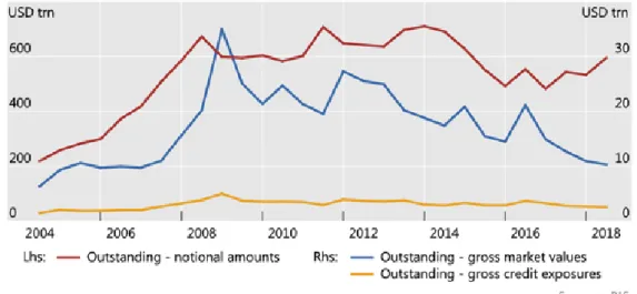
Table 1: Size and Market Value of OTC markets
1 The Bank for International Settlements (BIS) is an intergovernmental organization of central banks which "fosters international monetary and financial cooperation and serves as a bank for central banks." It is not accountable to any national government.
11
According to Table 1, there is a leverage effect. For instance, an agreement to buy 200 million USD with British pounds at a predetermined exchange rate in 1 year in OTC market. The total principal amount in this transaction is $200 million, but value of contract ought to be just $2 million.
According to Table 1, there is no an exponential shift on the OTC market like before the crisis. However, there is decrease in market size and value of global OTC market. This shows the effect of crisis and regulations to OTC market. The last detailed and updated information that is about the size of OTC derivative market is at Appendix 1. Furthermore, value of open interest of exchange traded markets is about USD 95.5 trillion. The last updated information about the size of exchange traded derivative market is at Appendix 2.
SECTION THREE
3. INSTRUMENTS OF RISK HEDGING 3.1.Forwards
3.1.1. Forward Contracts
Forward contract means a deal to purchase or sell an asset at a certain price for future time. It is opposite of spot contract that is an agreement to buy or sell an asset today. Financial institutions or a financial institution and its client use forward contracts and this shows that they are traded in the over-the-counter market.
If a dealer agrees to buy an asset at a specified certain price for a special future date, this is called “long position”. And if other dealer agrees to sell an asset at a same specified certain price for a same special future date, this is called “short position”.
12
Forward contracts on foreign exchange are well liked. Forward and spot foreign exchange traders are employed by many large banks. A foreign currency for sudden delivery is traded by spot traders. Delivery for a future time is traded by forward traders.
Table 2 enables quotes, which are for number of USD per GBP, on exchange rate between US dollar (USD) and British pound (GBP). It is ought to be made by a big international bank on May, 2010.
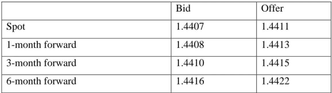
Table 2: Forward and spot quotes for the GBP/USD exchange rate, May 24, 2010 (GBP=British pound; USD= US dollar; quote is number of USD per GBP)
Bid Offer
Spot 1.4407 1.4411
1-month forward 1.4408 1.4413
3-month forward 1.4410 1.4415
6-month forward 1.4416 1.4422
First row demonstrates that at rate of $1.4407 bank is prepared to purchase GBP and it is prepared to sell GBP at a rate of $1.4411 in the spot market. Second row shows that bank is prepared to buy GBP in 1 month at a rate of $1.4408 and it is prepared to sell GBP at a rate of $1.4413. Third row points that bank is prepared to purchase GBP in 3 months at a rate of $1.4410 and it is prepared to sell GBP at a rate of $1.4415. Fourth row determines that bank is prepared to buy GBP in 6 months at a rate of $1.4416 and it is prepared to sell GBP at a rate of $1.4422.
Hedging foreign currency risk could be provided by using of forward contracts. An example of Hull (2012); on May 24, 2010, treasurer of a US corporation has information that is company will pay £1 million pounds in 6 months (i.e. on November 24, 2010) and wants to hedge against exchange rate moves. Using the quotes in Table 2 the treasurer can agree to buy £1 million 6 months forward at an exchange rate of 1.4422. The company then has a long forward contract on GBP.
13
It has agreed that on November 24, 2010, it will buy £1 million from bank for $1.4422 million. The bank has a short forward contract on GBP. It has agreed that on November 24, 2010, it will sell buy £1 million for $1.4422 million. Both sides have a deal.
3.1.2. Payoffs from Forward Contracts
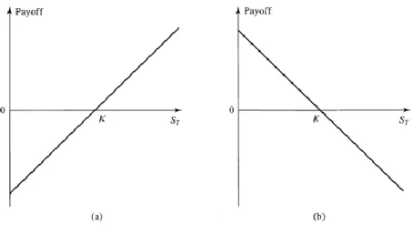
Figure 2:Payoffs from forward contracts; (a) long position, (b) short position. Delivery price=K; price of asset at contract maturity=ST
Before it is stated that company is obligated to buy £1 million for $1,442,200 due to forward contract. And there can be 2 different scenarios. For example, the spot exchange rate increased to 1.500 at end of 6 months and value of the forward contract is ($1,500,000-$1,442,200) = $57,800 to company. It would provide £1 million to be bought at an exchange rate of 1.4422 rather than 1.500. Or it is assumed that spot exchange rate decreased to 1.3500 at end of 6 months. Now, forward contract value is negative. ($1,350,000-$1,442,200)= -$92,200. Because, the contract would lead the company pay extra $92,200.
Basically, payoff from a long position in a forward contract on one unit of an asset is
14
Basically, payoff from a short position in a forward contract on one unit of an asset is
= K – ST
Where K is delivery price and St is spot price of an asset at maturity of contract. This payoffs or profit can be negative or positive. It can be easily seen at Figure 2. In the forward example, K=1.4422 and company has a long contract. When St=1.500, payoff is $0.0578 per £1; when St=1.3500, payoff is -$0.0922 per £1.
In a brief, people that think prices will go up takes a long position; people which thinks prices will go down, takes a short position
3.1.3. General Features of Forward Contracts
Forward transactions are done not on exchange traded markets, on OTC markets and they are done between financial institutions or a financial institution and its client.
Forward transactions can be done by helping different connection tools such as telephone, face to face.
Prices can change according to credibility of dealers. Forward transactions are not standardized.
Forward transactions cannot be assigned to third people.
Dealers must fulfill the obligations of contracts when maturity of contract is due date.
Forward transactions are usually divided two such as exchange rate forwards and interest rate forwards.
3.2.Futures
3.2.1. Futures Contracts
A future contract that is an agreement between two dealers to purchase or sell an asset at a certain price for a certain time in future is similar to a forward contract. However, future contracts are traded on exchange traded markets, not on OTC
15
markets. Dealers do not have to know each other, exchange traded market enables a guarantee that obligations in contract will be confirmed. Furthermore, one of most important things of a well working futures market is exchange center that is named “Clearing House”. Brokers fulfill the customers’ orders in this center.
It is stated before that futures contracts were traded are Chicago Board of Trade (CBOT) and Chicago Mercantile Exchange (CME), today emerged form of them is CME Group.
There are very kinds of commodities, which involve live cattle, sugar, wool, pork bellies, lumber, copper, aluminum, gold, tin etc., and financial assets, that include stock indices, currencies and Treasury bonds, form underlying assets in the various contracts.
Futures prices are also routinely reported in financial press. For instance, on October 1, January futures prices of copper are quoted as $3.5835. That is the price, exclusive of commissions, at which traders could agree to purchase or sell copper for January delivery. It is demonstrated same as other prices that are determined by the rule of supply and demand. Prices increase when more traders want to take long position, prices decrease when more traders want to take short position.
3.2.2. General Features of Futures Contracts
In a brief, the general features of futures contracts:
Future contracts are traded on exchange traded markets.
Parties on the contract are not responsible to each other, they are responsible to exchange center. So, there is no credit risk for two sides. Future contracts are standardized and they can be bought or sold until
16
The goods on the futures contracts must be homogenous, have raw material ability, prices of them should be determined in response to supply and demand, they can be stored, and the quality test of them could be easy. Moreover, the liquidity of goods on the futures contracts ought to be high.
In practice, futures contracts are done on agricultural products, natural resources, foreign exchanges, fixed interest rate debt tools and stock indices.
Moreover, futures contracts which are done on foreign exchanges, fixed interest rate debt tools and stock indices are called “financial futures contracts” in practice.
3.2.3. Standard Elements of Futures Contracts
Product, Security or Financial Indicator on The Contract Delivery Months
Delivery month is the date for cash agreement or physical exchange. Generally standard dates are determined like March, May, June, September and December periods. There can be different periods for different countries.
Contract Size
Contract size is minimum transaction amount of product in the contract. Delivery Arrangements
Delivery arrangement shows which way will be used on the due date, cash agreement or physical delivery.
Settlement Price
Settlement price is the price that is used in calculation of daily gain or loss and margin liabilities.
Maturity Date
Maturity Date is the last day for transaction on the contract. Margin Rates
Margin rate is the ratio that must be kept available at account for initial and continuous margins.
17 Tick Size / Minimum Price Movements
Tick size or minimum price movements are the minimum price movements. Daily Price Movement Limits
Daily price movement limits are the lower and upper limit for price of a future contract in a day.
Position Limits
Position limits are the maximum number of positions that are owned by a firm or an account.
3.3.Options
3.3.1. Option Contracts
Options can be traded both on over-the-counter and in exchange traded markets. An option generally includes the information below:
Type of Option: European or American Option
In European options, investor that buys the option has a right to sell or purchase only at the maturity date. In American options, investor that buys the option has a right to sell or purchase at any time (maturity date also can be possible). Moreover, European options do not mean they are sold in Europe or American options do not mean they are sold in USA. Today, two types of options are traded both on Europe and America.
Type of Contract: Call or Put Option
There are two kinds of options that are “call option” and “put option”. If investor that has the right to buy underlying asset at a certain price for a certain date in future, this situation is called “call option”. Moreover, if an investor that has the right to sell underlying asset at a certain price for a certain date in future, this situation is called “put option”.
Commodity or Security in the Option Contract: Stock, Bond etc. Premium of Option: Price of an Option
Price of option in the contract is the amount per share that an option buyer pays to the seller. Furthermore, most of options that are traded on exchanges are American. There are 100 shares to buy or sell in the contract in the exchange
18
traded equity option market. The analysis of European options is also easier than American options.
Option contracts are very similar to payment of insurance premiums. For example, houses and materials in the home are insured due to risks of theft or fire and so insurance premium is paid. If house is fired or materials in house are stolen, insurance company pays the loss of person who paid premium before. Now, a portfolio manager buys a put option to make loss at minimum due to negative changes or price declines in the spot market. This shows that house insurance is too similar to buying a put option.
Moreover, when a portfolio manager buys a put option, this transaction is called “portfolio insurance” in the literature of finance.
3.3.2. Payoffs from Options Contracts
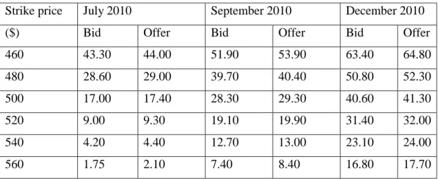
Table 3: Prices of Call Options on Google, June 15, 2010; stock price: bid $497.07; offer $497.25 (Source: CBOE)
Strike price July 2010 September 2010 December 2010
($) Bid Offer Bid Offer Bid Offer
460 43.30 44.00 51.90 53.90 63.40 64.80 480 28.60 29.00 39.70 40.40 50.80 52.30 500 17.00 17.40 28.30 29.30 40.60 41.30 520 9.00 9.30 19.10 19.90 31.40 32.00 540 4.20 4.40 12.70 13.00 23.10 24.00 560 1.75 2.10 7.40 8.40 16.80 17.70
Table 3 considers bid and offer quotes for a few of call options trading on Google. This table also demonstrates that the price of call option goes down when strike price goes up. There is a reverse proportion between them.
19
For example, it is assumed that an investor decides to buy a December call option contract on Google with an exercise price 520$. According to Table 3, offer price is $32, but this is a price for a share of option. It is also stated that options contracts are done with 100 shares in the USA. So, investor will have a cost $3200 and a right to purchase 100 Google shares for $520 each one. If the price does not increase above the $520 by 18th December, 2010, investor will have a
negative profit - $3200. Because, option is not exercised.
Or it is assumed that bid price of stock is $600. Consequently, investor will buy 100 shares at $520 and suddenly sell at $600 then profit is $8000, but when the initial cost of option is calculated, net profit is $4800.
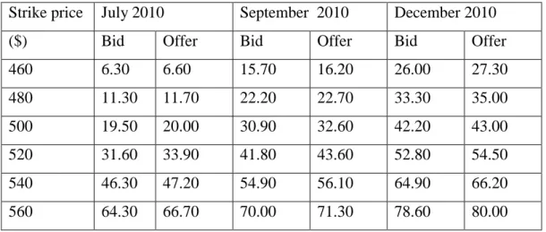
Table 4: Prices of Put Options on Google, June 15, 2010; stock price: bid $497.07; offer $497.25 (Source: CBOE)
Strike price July 2010 September 2010 December 2010
($) Bid Offer Bid Offer Bid Offer
460 6.30 6.60 15.70 16.20 26.00 27.30 480 11.30 11.70 22.20 22.70 33.30 35.00 500 19.50 20.00 30.90 32.60 42.20 43.00 520 31.60 33.90 41.80 43.60 52.80 54.50 540 46.30 47.20 54.90 56.10 64.90 66.20 560 64.30 66.70 70.00 71.30 78.60 80.00
Table 4 considers bid and offer quotes for a few of put options trading on Google. Moreover, this table determines that price of a put option increases when strike price rises. There is a directly proportional between them.
For example, it is assumed that an investor decides to sell a September put option contract on Google with an exercise price 480$. According to Table 4, bid price is $22.20 and with 100 shares on the contract, cash inflow is 100*$22.20= $2220. If the stock price of Google remains above $480, option is not exercised and
20
investor will have a profit $2220 at the end. However, when stock price of Google decreases to $420, then investor will have a negative profit ($420-$480)*100= $6000, but if initial profit is taken account, total loss or negative profit is $3780 (= -$6000+$2220)
Figure 3: Net profit per share from (a) purchasing a contract consisting of 100 Google December call options with a strike price of $520 and (b) selling a contract consisting of 100 Google September put options with a strike of $480.
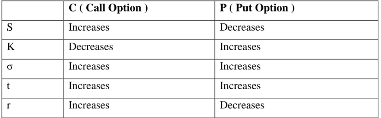
3.3.3. Basic Elements That Determine Option Prices
Cash Market Price of the Product on the Contract ( S ) Price of Option Usage ( K )
Volatility ( σ )
Remaining Time to Use the Option ( t ) Risk Free Rate ( r )
Table 5: The Effect of Basic Elements That Determines Option Prices to Option Premium
C ( Call Option ) P ( Put Option )
S Increases Decreases
K Decreases Increases
σ Increases Increases
t Increases Increases
21
3.3.4. Main Two Differences of Options from Forward-Futures:
There are two very important things to distinguish options from forwards and futures; an investor has a right to do something on option. But, investor does not have to exercise the right. Second one is that there is no cost to enter a forwards or futures contracts. However, there is a cost of getting an option.
3.4.Comparison of Forward-Futures-Option
Table 6: Comparison of Forward-Futures-Option
Basic Features Forward Futures Option
1) Tool for Hedging Risk Yes Yes Yes
2) Standard Contracts No Yes Yes
3) Exchange Traded / OTC OTC Exchange Traded
Exchange Traded and OTC
4) Physical Delivery Yes Generally No If right is used, Yes 5) Obligation for Margin Generally
No
Yes Yes for Seller
6) Cash Flow until Maturity Date
No Yes Yes for Seller
7) Credit Risk Yes No No
8) Leverage Effect There is no Importance
Yes Yes
9) Combination of Rights and Obligations
22
3.5.Types of Traders Which Make Transactions on Derivative Market
Traders are categorized to three such as hedgers, speculators and arbitrageurs.
3.5.1. Hedgers
Derivatives are used by hedgers to decrease the risk due to negative changes in the future. Investors take long position futures contracts to avoid price increments in the future. When investors have expectations of price decrements in future, they take short position of futures contracts.
Hedging transactions are used by portfolio managers, bankers in financial markets and they are also used by firms that use some goods like raw materials in goods markets. For instance, a portfolio manager can sell futures contracts on stock indices instead of selling portfolio stocks in the spot market to increase the performance of portfolio, to decrease the risks that are owned and to diversify portfolio. So, company cannot be affected by possible price decrements in the spot market. Moreover, especially foreign traders sometimes use futures markets products to hedge the risks that are originated by spot markets in developing countries.
Example: Hedging Using Options
It is assumed that a trader has 1000 Microsoft shares in May of 2004 and the share price is $28 for one share. Trader has a negative expectation for share prices in next 2 months and wants to be protected. Trader buys 10 July put option contracts at $27.5 strike price on CBOE. Now, trader has a right to sell 1000 shares with the price $27.5. Quoted option price is $1 and then each option contract will cost $100 (=100*$1), then total cost will be $1000 (=10*$100).
The cost of this hedging strategy is $1000, however it is guarantee that shares could be sold at minimum $27.5 for each share until maturity date of option. When market price of Microsoft shares go down of $27.50, option will be used
23
and $27500 will be gained. But, if initial cost is taken account, at total $26500 ($27500-$1000) will be gained.
But, when market price is above the $27.5, options will not be used. Net value of portfolio that is relevant with stock price of Microsoft is considered at Figure 4.
Figure 4: Value of Microsoft holding in 2 months with hedging and without hedging.
3.5.2. Speculators
Derivatives are used by speculators to bet the future market variables. Speculators have significant advantages in the futures markets due to leverage effect. Furthermore, transactions of speculators increase the liquidity of the market and volume of transactions, although they sometimes cause immediate price movements.
Example: Speculation Using Options
It is assumed that a speculator demonstrates that a stock will increase in 2 months, now in October. Current stock price is $20 and strike price $22.50 of a 2 month call option is sold now for $1. Two choices are showed in Table 8. Speculator also plans to invest $2000. First alternative is buying 100 shares and second one is buying 2000 call options that mean 20 call option contracts. It is assumed that
24
speculator is right and stock price increased to $27 in December. Profit of the first choice is 100*($27-$20) = $700. Second one’s gross profit is 2000*($27-$22.5) = $9000. But, if options premium is included net profit is $9000-$2000= $7000. In here, options are 10 times more profitable according to directly buying the stock. However, options can be cause more loss according to directly buying the stock. For example, stock price decreases to $15 in December. Profit of first choice is 100*($20-$15) = $500. If second choice is considered, option will not be exercised; this will cause a loss of $2000. Figure 5 demonstrates profit or loss of strategies.
These results show that options enable leverage like in futures. In options, good results become very good, but bad outcomes cause loss of all initial investment.
Table 7: Comparison of profits from two alternative strategies for using $2000 to speculate on a stock worth $20 in October.
December stock price
Investor’s strategy $15 $27
Buy 100 shares -$500 $700
Buy 2000 call options -$2000 $7000
Figure 5: Profit or loss from two alternative strategies for speculating on a stock currently worth $20
25
3.5.3. Arbitrageurs
Positions in two or more instruments are equalized by arbitrageurs to lock in a profit. Arbitrageurs aim to gain risk free profit with benefiting from price inequalities between markets. For example, if a good is traded in different regions, arbitrageur purchases good from the cheap place and sells good to expensive region and so risk free profit is gained. Similarly, when there is a different price from the price that should be included the transportation cost between spot and futures markets, arbitrageurs start to buy cheap region and to sell the expensive region, then markets are equalized. These transactions make the market to be real price. However, there is no way to get risk free profit with arbitrages in efficient markets.
3.6.Swaps
Swap means exchange. Swaps are financial transactions in which 2 parties change their payments with each other at a certain time period. The basic purpose of swaps is decrease the risk and uncertainty due to changes in interest rates and exchange rates with benefiting from different advantages of different markets of parties.
Generally, swaps provide financial managers to decrease risk and increase their revenue.
General reasons for swaps transactions:
Difficulties or easiness of reaching exchange rate funds.
Difficulties to obtain fixed interest rated funds versus easiness of getting variable interest rate funds.
Existence of different corporate and structural at different financial markets.
26
Counterparties in swap transactions are generally categorized into two groups that are fund users and brokers. Fund users make swap transactions because of decreasing the interest rate and exchange rate risk that are caused by economic and fiscal reasons. Brokers make swap transactions due to gaining commission and profit. Counterparties of swap transactions:
Enterprises
Financial companies International companies Agents that give loan credits Governments agents
3.6.1. Interest Rate Swaps
Two parties, that have different credit ratings, exchanges their interest rate payments which have different interest rate conditions, but at same amount. In interest rate swaps just interest rate payments due to debts are changed, capitals are not altered. Maturity is differs from 1 year to 15 years. General interest rate swap types are fixed-variable interest rate swaps, variable-variable interest rate swaps and variable-variable interest rate swaps.
3.6.1.1.Fixed-Variable Interest Rate Swaps
Counterparties have different credit ratings and they make the swap transaction with changing debts’ interest rates at same maturity and amount. With this transaction, one of counterparty gives up variable interest debts and it obtains a fixed interest debt structure. This protects itself to possible risks in future. Other counterpart, who has an expectation of decrease in interest rates in future, gives up fixed interest debts and it obtains a variable interest debt structure.
3.6.1.2.Variable-Variable Interest Rate Swaps
These types of swap are also known as “basis swap”. The aim is to benefit from differences in different variable interest rate markets. These swaps are used to
27
hedge or make arbitrage. For instance they are applied in between LIBOR and TIBOR, or in between USD PRIME RATE and LIBOR.
3.6.1.3.Fixed-Fixed Interest Rate Swaps
Fixed interest rate debts that are at different currencies are exchanged. The basic purpose is to decrease uncertainty and risk due to changes in foreign exchange rates.
3.6.2. Currency Swaps
This means the two money movements, which are in same amounts and are different currencies, are exchanged with a predetermined rate until maturity date, money are paid back to original owners after maturity date.
Main reasons for usage of currency swaps:
A corporation cannot find a loan with desired currency.
A corporation can find a lower cost loan with a different currency A currency swap could be implemented like:
a) Exchange of money
b) Changing and paying interest rates
c) Paying back capital money at maturity date.
3.6.3. Commodity Swaps
Reasons of companies for commodity swaps:
Protecting themselves due to price fluctuations Closing the open positions related to commodities.
Commodity swaps are especially used in petroleum futures contracts to 5 years. This method means counterparties change fixed and variable price of a commodity, which is determined amount and quality, with a contract in a determined period. Furthermore, both producers and consumers protect themselves due to price movements with this application.
28
3.7.New Generation Derivatives 3.7.1. Warrants
Warrants, which are organized after bond issues, are a kind of call options. Maturity long of warrants is usually a year.
After warrants are organized, they can be bought or sold apart from bonds in some situations.
3.7.1.1.Stock Warrants
A corporation, that has N stocks on circulation, issues M warrants. Each warrant includes a right to buy Y stocks.
This buying right is given at time T and at price X.
If the net asset value of company is V and if warrant owner uses right of buying, cash inflow to the company will be equal to MYX.
The net asset value of company goes to V + MYX
The net asset value of company will be divided to (N + MY) stocks. After usage of warrant, immediately stock price will be (V + MYX) / (N +
MY)
The amount that will go to warrant owner: Y [(V + MYX) / (N + MY) – X]
If this amount positive (+), warrant is used; reverse warrant is not used.
3.7.2. Exotic Options
Exotic options are organized to compensate the specific needs of companies.
They have more complex structure than classical European and American option types.
29
3.7.2.1.Types of Exotic Options
They are not transacted in stock market exchange. They come to forefront with creative attributes.
Types of Exotic Options: Equity collars Equity warrant
Chooser option-as you like it Compound options on options Installments options Pay-later options Asian options Barrier options Lookback options Rainbow options Basket options Quantos
Forward start options etc.
3.7.3. Futures Options
The asset, which is subject of the option, is futures contracts in these types of options. The most popular examples are options organized on treasury bills futures contracts in CBOT and options organized on Eurodollar futures contracts.
30
SECTION FOUR
4. FINANCIAL DERIVATIVE PRICING MODELS
4.1.Forward Pricing Model
The formula of a forward pricing is like:
It is assumed that a forward contract on an investment asset at price S0 that
enables no income. r= risk free rate T= time to maturity F0= forward price
Example: It is assumed that a long forward contract to buy a non-dividend paying
stock in 3 months. Current stock price is $80 and risk free rate is 5% is per year. Situation 1:
If forward price is too high at $90. An arbitrageur could borrow $80 and r= 5 % per year, buy a share and short a forward contract to sell a share in three months. Arbitrageur gets $90 from selling the share after 3 months. Sum of money required to pay the debt:
80*e^ (0.05*3/12) = $81
So, arbitrageur gets $90-$81 = $9 profit.
Situation 2:
If forward price is too low at $70. An arbitrageur can short a share, makes a short sale at 5% risk free rate per year, for 3 months and gets a long position in a 3 months forward contract. The cost of short sale is 80*e^ (0.05*3/12) = $81 in 3 months. However, arbitrageur pays $70 and then net profit is $81-$70= $9 at end of 3 months.
31
4.2.Futures Pricing Models 4.2.1. Cost of Carry Model
Pricing of futures contracts is based on Cost of Carry Model. This model is used to determine value of futures contracts on products that are not financial. It also used in determining value of future contracts on financial products.
The model measures the relationship level between price of products or financial assets and futures price. Futures price should be higher than cash price at any time period before delivery time. Because, there is a cost of carry. Cost of carry includes:
Cost of financing to purchase (interest rate cost) Stock cost
Insurance cost Freight cost
Potential other costs when carrying period The model is formulized like:
Futures Price = Cash Price + Unit Financing Cost + Unit Stock Cost Fct = St +(St * Rt,T*(T-t)) / 365 + Gt,T
Fct =Futures price at time t , that will be delivery at T.
St = Cash price at time t
Rt,T = Risk free rate that can be loaned at time t for T-t period
Gt,T = Stock cost of the product at period T-t
This model is valid when some assumptions are applied. They are:
There should not be the cost of information or transaction that can affect buying or selling the quantity of product or futures contract.
There should not be any restriction on the amount of lending or borrowing. Lending or borrowing rate should be done on same risk free rate.
There should not be any margin risk.
There should not be a change in features of products until maturity date. There should not be taken any tax.
32
Relationship between cash price and futures price can be formulized in Cost of Carry Model as:
Cost of Carry = Futures Price – Cash Price
In developed futures markets, there is no difference between futures price that is occurred and futures price that is calculated theoretically. First reason of that is the efficiency level of market is too high. Second reason is that arbitrage facility prevents this difference.
Consequently, arbitrage relationship between cash and futures market is very important to price future contracts.
Example:
Purpose: buying a C. gold after a month. How can it be bought?
An agreement now and buy the gold at F price at end of month.
Loan can be taken now, can be purchased the gold and loan can be paid at end of month.
Situation is same for two choices. These two alternatives mean different portfolios, but the result is same and so costs should be same.
Spot price = TL 300
Interest rate per month = 1% Expiration date = 1 month
2nd choice: A loan is taken at TL 300 and gold is bought for TL 300… Loan is paid at end of month. 300*1.01 = 303 TL After transactions a gold is bought and TL 303 is paid.
Two portfolios have same results; this means gold price after a month is TL 303. Arbitrage facility with different price:
Situation 1:
33
A futures contract is sold (short position). TL 300 is loaned from bank and a gold is boght at TL 300. Then futures contract is sold at TL 305 after a month and the loan TL 303 is paid and then profit is TL 2 (= TL 305 - TL 303)
Situation 2:
If price is not TL 303, it is TL 300:
Gold is short sold and futures contract is bought to close it. TL 300 is deposited at bank. Value of money is TL 303 after a month. TL 300 is paid for future contract. Net profit is TL 3 (= TL303 – TL 300)
Two situations show the arbitrage. So, futures price should be at TL 303 not to be an arbitrage.
4.2.2. Stock Indices Model
A significant feature is taken account in determination the value of stock indices futures contracts in developed country stock markets. The important feature is that two different portfolio investments are equivalent. First portfolio is consisted with buying assets that forms the indices. Second portfolio is consisted with purchasing stock indices futures contracts and stocking treasury bills whose value is equal to initial value of indices.
1st way: Value of indices at the end of period + Dividend payment
2nd way: (Value of indices at the end of period – Value of indices that is considered in contract) + Value of T bill at the end of period.
Et : Value of indices at initial date of period
Et+1 : Value of indices at end of period
Es : Futures price of indices in contract
T : Dividend payment
HBt+1 : Value of T bill at end of period.
r : Effective interest rate d : Dividend Yield
34
Derivation of futures price of indices is showed below step by step:
1. Et+1 + T = Et+1 - Es + HBt+1 (Value of 1st portfolio at end of period =
Value of 2nd portfolio at end of period)
2. T = - Es + HBt+1 3. HBt+1 = (1+r)* Et 4. T = - Es + (1+r)* Et 5. Es = (1+r)* Et – T 6. d= T / Et => T= Et * d 7. Es = (1+r)* Et - Et * d
8. Es = Et + (r-d)* Et (General Formula of Futures price of indices)
Example:
Et = TL 23000
r= 80 % (with simple interest rate 20 % for 3 months) d= 16 % (4 % for 3 months)
Date= 3 months
Es = Et + (r-d)* Et => Es = 23000 + (0.20-0.04) * 23000
Es = TL 26680
The proof of stock indices futures pricing method is below: Cost of Debt for 3 months = 80% * 23000 * (90/360) = TL 4600 Dividend Yield for 3 months = 16% * 23000 * (90/360) = TL 920 Balance Contract Price is = 23000 + 4600 – 920 = TL 26680
In addition to above explanations and example, formula of theoretical exchange rate futures pricing is like
4.3.Option Pricing Models 4.3.1. Black and Scholes Model
In the world, Black and Scholes Model, is developed by Fischer Black and Myron Scholes in 1973, consists the basic of most of derivative pricing models. The Black-Scholes model is one of the most commonly used models to price European
35
calls and puts. It serves as a basis for many closed-form solutions used for pricing options. The standard Black-Scholes model is based on the following assumptions:
There are no dividends paid during the life of the option. The option can only be exercised at maturity.
The markets operate under a Markov process in continuous time. No commissions are paid.
The risk-free interest rate is known and constant.
Returns on the underlying stocks are log-normally distributed.
The basis of the model is to make a portfolio that has a return of risk free rate with taking a long position at call option account and taking a short position at put option account. It is arbitrage theorem with a different point of view.
The value of call option, C, is calculated like: C = SN * d1 – K * (e^ (-rt)) * Nd2 =>>
d1 = ln(S/Ke^ (-rt)) / σ (t^1/2) + 0.5 σ(t^1/2)
d2 = d1 - σ (t^1/2)
ln = natural logarithm
N (.) = cumulative probability distribution function for standard normal variables S= Cash Market Price of the Product on the Contract
K= Price of Option Usage σ= Volatility
t= Remaining Time to Use the Option r= Risk Free Rate
All the variables are expressed above. Four factors that are desired for model can be easily gathered. However, only volatility (σ) cannot be calculated exactly.
The value of put option, P can be calculated with using the pricing relationship between call option and put option (put-call parity).
36
If relationship between values of call and put options remove, then there will be an arbitrage opportunity.
When pricing relationship between call-put options and value of call options are combined, the value of put option is calculated like:
P= Ke^ (-rt) * (1 – Nd2) – S * (-Nd1 + 1)
Moreover, Morton developed the Back and Scholes Model. Morton did not use capital asset pricing model (CAPM) in his technique while Black and Scholes had used CAPM model to price options.
4.3.2. Addition to Option Pricing-Factors that affect the Option Premium
Black Scholes Model is demonstrated in previous parts. It is not easy to understand the model and to calculate without a calculator. So, knowing how to comment factors affecting the option premium will be beneficial, instead of knowing details of how model works. Because, there are many calculators that calculates option premiums according to this model on internet or stock market websites.
Basic elements that affect the option premium are stated before, but not in detail. Now, direct factors affecting option premium, possible changes with these factors will be considered.
Firstly, main content of an option premium is intrinsic value and time value. Factors of Intrinsic Value: Factors of Time Value:
Type of option (Call/Put) Time to maturity Underlying Asset Price Volatility rate
Strike Price of Option Risk free interest rate
Dividend ( valid for just equities and equity indexes)
37
For instance, at maturity date, a call option with an underlying asset price of TL10 and strike price of TL9, so intrinsic value is TL1. Another example is a put option with a strike price of TL11 and an underlying asset price of TL10, so intrinsic value is TL1.
In addition to intrinsic value, more important thing in option pricing is to know option has how much time value. Moreover, with maturity date, options have no time value and their premium is calculated according to just their intrinsic value.
Now, factors of option’s time value that affect the option premium are below to understand premium of options before maturity date.
4.3.2.1.Remaining Time to Maturity
If maturity of an option is long, then volatility probability of underlying asset and movement probability of option with a profit way to beneficiary increase. This also raises the value of option. Because, said probabilities increase the probability loss of seller investor. Consequently, seller investor demands extra premium and then price of option raise.
Moreover, when maturity of option closes, said risks decline and so they prefer to sell more and they decrease price of options. So, with this logic when maturity of option closes, time value of option decreases fast.
38
Furthermore, time value of intrinsic value, non-intrinsic value and breakeven options have different contributions to their premiums. Much of high intrinsic value option premiums are covered by intrinsic value, so time value is little in premium of these types of options. In addition, very non-intrinsic value options are very far from their intrinsic value, so probability of being intrinsic value is nearly zero, so time value of options is little due to very low premium. Moreover, many probabilities can be occurred in breakeven options. So, options are sometimes intrinsic value and sometimes non-intrinsic value options and their probability to be intrinsic or non-intrinsic contributes positively to their premium. Time to maturity mostly affects premium of breakeven options.
4.3.2.2.Volatility Ratio
Volatility means that price of underlying asset goes up or down from its price level in a specified time. For instance, volatility rate is stated like 10%; it can be understood that price of underlying asset can go up or down to 10% from its level.
When volatility increases, premium of options raises in which it is not important call or put options. When it volatility decreases, it declines.
There are two types of volatility such as historical volatility, which is calculated according to historical price movements, and implied volatility, in which future volatilities are reflected in it. Implied volatility is used in options market.
Implied volatility of high intrinsic value options or low intrinsic value options are much than implied volatility of breakeven options. For instance, in the Figure 6, there is call option in graph. Strike price increases to right and when strike price of call option raise, it becomes more non-intrinsic value options.
Call option is high intrinsic value and high non-intrinsic value when strike price is very low or very high. Consequently, implied volatility is high. Implied volatility is very low in breakeven point. Same situation is valid for put options.
39 Figure 7: Implied Volatility Rate
4.3.2.3.Risk-free Rate
Increase in risk free rate decreases the present value of option strike price. So, it increases call option premium. This also means lower strike price.
Increase in risk free rate decreases the premium of put option and strike price declines. So, premium price of put option decreases.
4.3.2.4.Dividend
Dividend is a variable that is just accounted in index options and equity options. Dividend causes decrease in price of equity. So, a call option premium that is occurred by an index including dividend payer companies is lower than a call option premium that is occurred by an index involving no-dividend payer companies. Consequently, dividend decreases the call option premium.
However, dividend payment increases the value of put option premium. Because, when company pays dividend, value of equity (underlying asset) decreases and this also increases put option premium.