Potential information and target variables for UK monetary policy

(1)

Full Terms & Conditions of access and use can be found at

http://www.tandfonline.com/action/journalInformation?journalCode=raec20

Download by: [Bilkent University] Date: 27 October 2017, At: 01:32

Applied Economics

ISSN: 0003-6846 (Print) 1466-4283 (Online) Journal homepage: http://www.tandfonline.com/loi/raec20

Potential information and target variables for UK

monetary policy

Hakan Berument & Richard T. Froyen

To cite this article: Hakan Berument & Richard T. Froyen (1998) Potential information and target variables for UK monetary policy, Applied Economics, 30:4, 449-463, DOI: 10.1080/000368498325723

To link to this article: http://dx.doi.org/10.1080/000368498325723

Published online: 04 Oct 2010.

Submit your article to this journal

Article views: 21

View related articles

(2)

1_{Chrystal and MacDonald (1994) study the relationship between income and two monetary aggregates for the United Kingdom. Sims} (1992) studies the money± income relationship for the G7 countries.

Potential information and target

v

ariables

for UK monetary policy

H AKAN BE RU MEN T and RIC HARD T. FR OY EN³

Bilkent University, Ankara, Turkeyand³_{Department of Economics, CB}_# _{3305, Gardner}

Hall, University of North Carolina, Chapel Hill, NC 27599-3305, USA

The relationship between traditional monetary policy goal variables (nominal GDP, real GPD and the in¯ ation rate) and a number of ® nancial market variables is investigated. The question examined is which if any of these ® nancial market variables (monetary aggregates, interest rates and interest rate spreads) are potentially useful as either information variables or intermediate targets. While the implications concern-ing the usefulness of the ® nancial variables considered are pessimistic concernconcern-ing nominal GDP, more robust relationships are found for real GDP and in¯ ation. The latter ® nding is of interest given the current UK monetary policy strategy of in¯ ation targeting. Our results are, however, more supportive of the usefulness of several ® nancial variables as information variables than as intermediate targets.

I. INTRO DU CTIO N

Monetary authorities in industrialized countries have em-ployed a number of ® nancial variables as either intermedi-ate targets or information variables. This study investigintermedi-ates the relationship in the United Kingdom between nominal GDP, real GDP, in¯ ation and a number of possible mone-tary policy target or information variables. In particular, we are interested in ® nding out which relationships remained stable over the years since 1979, a period of rapid innova-tion in ® nancial markets. The quesinnova-tion is of interest because only variables which have stable relationships with income and/or in¯ ation are capable of playing important roles in monetary policy formation, a point on which we elaborate below.

There have been numerous studies of the money± income relationship in the United States and United Kingdom (as well as in other countries). Friedman and Schwartz (1982) is a noteworthy study of relationships among money, income and interest rates in the two countries over the past century. In recent years there have been a number of studies for the United States using vector autoregression and/or cointegra-tion techniques to study the relacointegra-tionship between income (both nominal and real) and a number of ® nancial variables: Bernanke and Blinder (1992), Feldstein and Stock (1994),

Friedman and Kuttner (1992), (1993), Ramey (1993) and Stock and Watson (1989).1 _{The results from these studies}

di er in signi® cant respects. A ® nding of several recent studies (Friedman and Kuttner, 1992; 1993) is that the relationships between income (both real and nominal) and

all the monetary aggregates break down in the 1980s.

Fried-man and Kuttner (1992) also ® nd that monetary aggregates lose predictive power with respect to in¯ ation in the post-1979 period.

These studies ® nd that the income± interest rate relation-ship does not deteriorate, but rather becomes stronger in the 1980s. They also ® nd that a measure of the public± private interest rate spread has signi® cant predictive power with respect to nominal and real GDP. With respect to in¯ ation, Friedman and Kuttner (1992) ® nd that interest rates lose their predictive power in the post-1979 period, while the interest rate spread generally has no predictive power.

With respect to the money-income relationship Ramey (1993) and Feldstein and Stock (1994) come to a di erent conclusion. They ® nd that for the M2 aggregate the money± income relationship remains robust with inclusion of data from the post-1979 period.

Our research examines whether there is evidence of any stable relationships between income and/or in¯ ation and a number of ® nancial variables in the United Kingdom. We

0003± 6846 Ó 1998 Routledge 449

(3)

2_{Variance decompositions, of course, have there own drawbacks including dependence on the ordering of the variables.}

3_{As noted in the introduction, Bernanke and Blinder (1992) and Friedman and Kuttner (1992) ® nd that the public± private spread,} measured for the United States by the treasury bill± commercial paper rate spread has predictive power with respect to income. Movements in this spread are interpreted as measures of a risk premium or of credit rationing. Other research has focused on the spread between the federal funds rate and treasury bill rate as a measure of monetary policy stance. Moersch (1996) shows that this spread has predictive power with respect to industrial production in both the United States and United Kingdom (where the overnight interbank rate replaces the federal funds rate). We use the base bank lending rate minus the bill rate as a measure of the public± private spread and the call (overnight) rate minus the bill rate as a spread that measures the stance of monetary policy.

4_{The monetary base is used only in a limited number of our tests due to several breaks in this data series.}

look to see if there have been shifts in these relationships of the same type as in the United States. As noted above, relationships between income (or in¯ ation) and various potential monetary policy targets or information variables are of importance in the design of an optimal monetary policy strategy. As Friedman and Kuttner (1992, p. 473) point out concerning monetary aggregates

From an information-variabl e perspective there is no point to the central bank reacting to ¯ uctuations in money if those ¯ uctuations bear no implications for sub-sequent movements in income and prices. From an inter-mediate-target perspective, there is even less point to making monetary policy as if controlling money were stochastically equivalent to controlling income and prices if in fact there is no relationship between them.

Which variables then, if any, are good candidates as mone-tary policy targets or information variables in the United Kingdom?

Our answer to this question is, in brief, that a number of ® nancial variables do appear to have relationships with ultimate monetary policy goals that make these ® nancial variables useful in policy formation. Our results indicate, however, that the role of these ® nancial variables might more usefully be as information variables rather than as intermediate targets, for reasons that will be explained.

The paper is organized as follows. Section II explains the procedures we employ and examines the time series proper-ties of the data. Section III presents the results of tests based on vector autoregressions. Section IV summarizes these results and further examines their implications for policy. Section V contains concluding comments.

II . STATI STICAL PRO CEDU RES AN D TIM E SERIES PRO PERTIES O F THE DA TA

Procedures

Granger causality is one criterion that has been widely employed in tests of money± income and money± in¯ ation relationships. It is an appropriate methodology with regard to the choice of an information variable because there the concern is whether or not a given ® nancial magnitude has predictive power with respect to a target variable. As Fried-man and Kuttner (1992, p. 474) observe, this is the relevant

criterion `regardless of whether the information it contains re¯ ects true causation, reverse causation based on antici-pations, or mutual causation by some independent but unobserved in¯ uence’.

With regard to the choice of an intermediate target, however, the distinction made by Bernanke (1993) between the structural question and the forecastingquestion is

rel-evant. Granger causality analysis is useful in answering the forecasting question. If, however, a ® nancial variable is Granger causal with respect to a goal variable due, for example, to mutual causation by a third variable it would not be a desirable intermediate target. Once the central bank began to control the variable, its relationship with the third variable, and thus with the goal variable would break down; Goodhart’s law would come into play.

Further information on whether the relationship between a given ® nancial variable and income or in¯ ation is struc-tural, in the sense that it is important in the transmission mechanism of monetary policy actions, can be gained from variance decompositions. These are constructed from or-thogonalized residuals and at least avoid `third variable causality e ects’ for variables included in the VAR. By changing the set of included variables one can check for other `third variable’ e ects.2

A third type of relationship that we explore between income or in¯ ation and several ® nancial variables is that of cointegration. There may exist long-run equilibrium rela-tionships between ® nancial variables and income and/or in¯ ation which have important policy implications as dis-cussed in Friedman and Kuttner (1992). Cointegration be-tween a given monetary aggregate and nominal income would, for example, imply that `base drift’ should be avoided in targeting the aggregate because velocity disturbances are transitory. Moreover, the existence of cointegration among the variables in our system has implications for the proper speci® cation of tests for short-run relationships among them.

Time series properties of the data

The ® nancial variables we include in our VARs and cointe-gration tests are a monetary aggregate, chosen amongM0

(the monetary base),M2andM4; an interest rate, either the treasury bill rate (RB) or call money rate (RC); or an interest

rate spread, either the call rate minus the bill rate or the base bank lending rate (RL) minus the bill rate.3 , 4 Additionally, in

some of our VARS we include a measure of government

(4)

5_{The Appendix containing additional Tables is available from the authors on request.}

6_{The UK in¯ ation rate does appear to be highly autocorrelated. In a regression of in¯ ation on its ® rst ® ve lagged values the sum of the} coe cients is 0.85 and the value of the Ljung± Box Q-statistic is 185.2 (p value

=

0.00).

7_{Both tables report results of cointegration tests performed without the inclusion of a deterministic time trend. We have computed the} same statistics with a trend included, with no substantive e ect on the results. (These test results are given in Table A2 and A3, available from authors on request.)

expenditures (G). As goal variables we consider nominal GDP and then, separately, real GDP (RGDP) and consumer price in¯ ation (Pd). Data are quarterly for 1957 : 1± 1993 : 4, though sometimes a shorter period is considered due to data unavailability; details are given in footnotea_{to Table 1. In}

addition to considering this whole period we consider two subperiods: 1957 : 1± 1979 : 2 and 1979 : 3± 1993 : 4. The breakpoint in 1979 is chosen because it marks the shift in policy with the election of Margaret Thatcher which a ected monetary and bank regulatory policy.

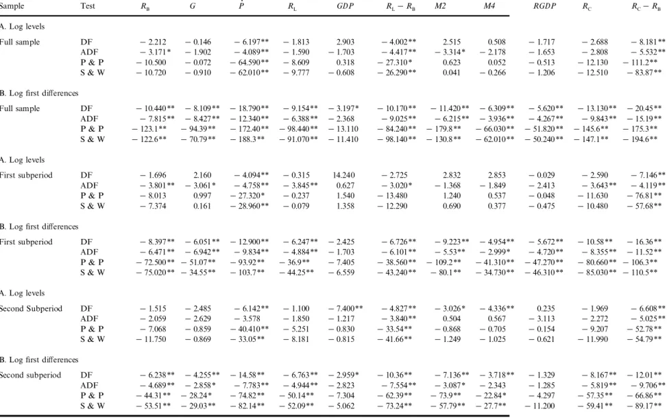
We begin by testing the series for the presence of unit roots. We use four tests: the Dickey± Fuller test (DF), the augmented Dickey± Fuller (ADF) test and the tests pro-posed by Phillips and Perron (1988) (P and P) and Stock and Watson (1988) (S and W). Table 1 reports results from these tests. Panels labelled A show test results where all series are expressed in log levels except for interest rates and interest rate spreads which are levels and the in¯ ation vari-able which is the log ® rst di erence of the price level. A trend was not included in these tests. (Results including a deter-ministic time trend are given in Table A.1 of the appendix.5₎

With the exception of the in¯ ation rate and interest rate spreads, these tests do not consistently reject the hypothesis of a unit root in the series using the four respective methods. Each panel labelled B shows the results of the same unit root tests after di erencing the logs (the level in the case of the interest rate) of the variables (therefore second di erenc-ing of the price level). The hypothesis of a second unit root is decisively rejected for almost all the series. An exception is the nominal GDP series where only the Dickey± Fuller test rejects the presence of a unit root and only for the whole period and second subperiod. The presence of a second unit root in the in¯ ation rate and log ® rst di erence of real GDP, the components of the log ® rst di erence of GDP, is rejected in all cases except the second subperiod for real GDP. Thus the evidence seems most consistent with stationarity of the ® rst di erence of GDP.

The results in Table 1 indicate that the log levels (or levels in the case of interest rates) of all the series we examine with the exception of interest rate spreads and the in¯ ation rate are nonstationary. There may, however, be stationary rela-tionships among those that are nonstationary; cointegrating vectors may exist.

Cointegration requires the stationarity of a linear combi-nation of nonstationary series. For example, if the logarithm of money (M), income (Y) and an interest rate (R) are individually nonstationary but they follow a simple linear relation such as

Y

-

a

-

b M

-

g R (1)

and this relationship is stationary for nonzero values of

b andg jointly, then these three variables are cointegrated. If the equation is stationary, this suggests that following dis-turbances to M, Y or R there will be an adjustment to restore the equilibrium relationship among these variables. We investigate the presence of cointegration among the nonstationary variables in our system using the Johansen procedure. The variables included in the ® rst system we consider are nominal GPD, a monetary aggregate (M2 or

M4), a short-term interest rate (R_C) or, alternatively, one of the two interest rate spreads. The second system is a four-variable system where nominal GDP is replaced by separate real GDP and in¯ ation (Pd) measures.

The inclusion of the GDP measures and monetary ag-gregates in tests for cointegration requires no explanation. Inclusion of the other time series does. Consider ® rst the inclusion of the in¯ ation rate which from Table 1 appears to be a stationary variable. Hansen and Juselius (1995), how-ever, suggest that there are cases when it is useful to include stationary variables in applying the Johansen procedure. As they explain, `Often, a stationary variable might a priori play an important role in a hypothetical cointegration relation, for instance, an in¯ ation rate. In particular, variables with a high degree of autocorrelation, also called near-integrated variables, are often very important in establishing a sensible long-run relation.’6

Next consider the nominal interest rate (RC)[or

alterna-tively RB, (see footnote 5)]. The test statistics in Table 1 do

not reject the presence of a unit root in any of our interest rate measures. But if, as indicated by Table 1 in¯ ation is I(0), then if the nominal interest rate is I(1), the real interest rate must be I(1) which is inconsistent with many conventional macroeconomic models. King et al. (1991), ® nd evidence that for US data the real interest rate is nonstationary and give a real business cycle interpretation to this result. An alternative possibility is that although we cannot reject the possibility of a unit root in the interest rate series, they are in fact stationary though near-integrated. If the nominal inter-est rate is I(1), it should clearly be included in applying the Johansen procedure; if it is instead a near integrated vari-able the rationale for its inclusion would parallel that for in¯ ation. The latter rationale also applies to the inclusion of interest rate spreads.

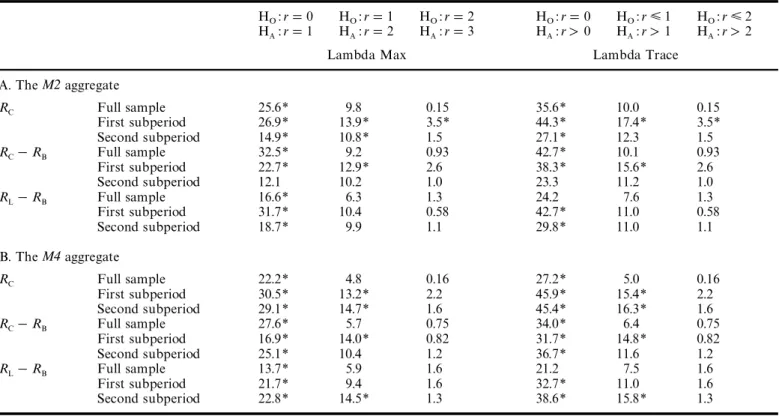
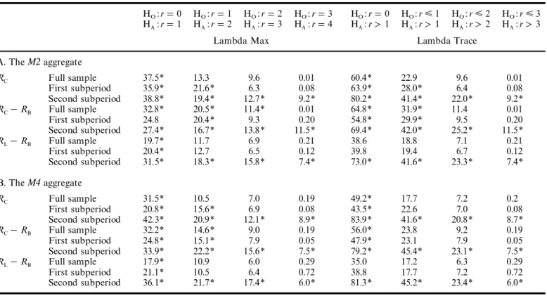
Table 2 reports values of Johansen’s lambda max and trace statistics for a number of three variable systems. Table 3 presents the same statistics for systems where nominal GDP is replaced by real GDP and the in¯ ation rate is added.7 _{The lambda max statistic tests the null hypothesis}

of r cointegrating vectors against the alternative hypothesis

(5)

Table 1. Stationarity tests for selected variablesa,b Sample Test R_B G Pd R_L GDP R_L- R_B M2 M4 RGDP R_C R_C- R_B A. Log levels Full sample DF - 2.212 - 0.146 - 6.197** - 1.813 2.903 - 4.002** 2.515 0.508 - 1.717 - 2.688 - 8.181** ADF - 3.171* - 1.902 - 4.089** - 1.590 - 1.703 - 4.417** - 3.314* - 2.178 - 1.653 - 2.808 - 5.532** P & P - 10.500 - 0.072 - 64.590** - 8.609 0.318 - 27.310* 0.623 0.052 - 0.513 - 12.130 - 111.2** S & W - 10.720 - 0.910 - 62.010** - 9.777 - 0.608 - 26.290** 0.041 - 0.266 - 1.206 - 12.510 - 83.87** B. Log ® rst di erences

Full sample DF - 10.440** - 8.109** - 18.790** - 9.154** - 3.197* - 10.170** - 11.420** - 6.309** - 5.620** - 13.130** - 20.45** ADF - 7.815** - 8.427** - 12.340** - 6.388** - 2.368 - 9.025** - 6.215** - 3.936** - 4.267** - 9.843** - 15.19** P & P - 123.1** - 94.39** - 172.40** - 98.440** - 13.110 - 84.240** - 179.8** - 66.030** - 51.820** - 145.6** - 175.3** S & W - 122.6** - 70.79** - 188.3** - 91.070** - 11.410 - 98.140** - 130.8** - 62.010** - 50.240** - 147.1** - 194.6** A. Log levels First subperiod DF - 1.696 2.160 - 4.094** - 0.315 14.240 - 2.725 2.832 2.853 - 0.029 - 2.590 - 7.146** ADF - 3.801** - 3.061* - 4.758** - 3.845** 0.627 - 3.020* - 1.368 - 1.849 - 2.413 - 3.643** - 4.119** P & P - 8.013 0.997 - 27.320* - 0.237 1.540 - 13.480 1.240 0.537 - 0.048 - 11.630 - 76.81** S & W - 7.374 0.161 - 28.960** - 0.079 1.358 - 12.290 0.690 0.377 - 0.475 - 10.480 - 57.68** B. Log ® rst di erences

First subperiod DF - 8.397** - 6.051** - 12.900** - 6.247** - 2.425 - 6.726** - 9.223** - 4.954** - 5.672** - 10.58** - 16.36** ADF - 6.471** - 6.942** - 9.834** - 4.884** - 1.703 - 6.101** - 5.53** - 2.999* - 4.720** - 8.355** - 11.52** P & P - 72.500** - 51.07** - 93.92** - 36.9** - 7.405 - 38.560** - 109.2** - 41.310** - 47.270** - 80.660** - 106.3** S & W - 75.020** - 34.55** - 103.7** - 44.25** - 6.559 - 43.240** - 80.1** - 34.730** - 46.310** - 85.030** - 110.5** A. Log levels Second Subperiod DF - 1.515 - 2.485 - 6.142** - 1.100 - 7.400** - 4.827** - 3.026* - 4.336** 0.235 - 1.969 - 6.608** ADF - 2.059 - 2.629 - 3.578 - 1.850 - 1.217 - 3.840** 0.504 0.567 - 3.113 - 2.272 - 5.025** P & P - 7.068 - 0.859 - 40.410** - 5.251 - 0.830 - 33.54** - 0.868 - 0.705 - 0.154 - 9.207 - 52.78** S & W - 11.750 - 0.869 - 33.05** - 8.181 - 0.815 - 41.66** - 1.249 - 1.025 - 0.621 - 11.990 - 54.79** B. Log ® rst di erences

Second subperiod DF - 6.238** - 4.255** - 14.58** - 6.763** - 2.959* - 10.36** - 7.136** - 3.718** - 1.329 - 8.167** - 12.01** ADF - 4.689** - 2.858* - 7.783** - 4.944** - 2.823 - 7.554** - 3.087* - 2.343 - 1.285 - 5.819** - 9.706** P & P - 44.31** - 28.24* - 74.82** - 50.14** - 7.304 - 62.39** - 73.9** - 22.84* - 4.297 - 57.35** - 66.86** S & W - 53.51** - 29.03** - 82.14** - 52.09** - 5.062 - 73.24** - 57.79** - 27.7** - 11.200 - 59.41** - 89.17**

a_{The longest sample period is 1957 : 1± 1993 : 4 but many of the series are only available for shorter periods as noted below. The source for all the data is either the OECD Main Economic Indicators}

data tapes or the IMF-IFS tape. All data are quarterly values except for M4 which is the ® rst month’s value for each quarter. Series available for less than the full period and dates of availability and data source are as follows: The treasury bill rate (RB), 1957 : 1± 1992 : 4, IMF; loan rate (RL), 1966 : 3± 1993 : 4, IMF; call money rate (RC), 1960 : 1± 1994 : 1, OECD; M2, 1957 : 2± 1993 : 4, IMF; M4,

1963 : 3± 1994 : 3, OECD; nominal GDP, 1963 : 1± 1993 : 4, IMF; real GDP (RGDP), 1957 : 1± 1992 : 2, IMF; change in the log of the consumer price index (P), IMF; 1957 : 2± 1992 : 4. The breakpoint between the ® rst and second subperiods is 1979 : 2.

b_{The critical values for both DF and ADF tests are} - _{2.89 for n}=_{100 and} - _{2.93 for n}=_{50 for 5% and} - _{3.51 for n}=_{100 and} - _{3.58 for n}=_{50 for 1%, where n is sample size.The critical values}

for the P&P tests are - 20.49 for 5% and - 28.32 for 1%. The critical values for S and W tests are - 14.1 for 5% and - 20.6 for 1% level of signi® cance. The critical values for the DF and ADF tests are from Harvey (1990), for the S and W test from Stock and Watson (1988), and for the P&P test from Phillips and Ouliars (1990).

2 H

.B

er

um

en

t

an

d

R

.

T

.F

ro

ye

n

(6)

Table 2. Johansen’s cointegration tests among3variables: GDP,M2or M4, and RC, RC

-

RB, or RL

-

RB(without trend)

RB Full sample 13.7* 5.9 1.6 21.2 7.5 1.6 First subperiod 21.7* 9.4 1.6 32.7* 11.0 1.6 Second subperiod 22.8* 14.5* 1.3 38.6* 15.8* 1.3

*Indicates signi® cance at 10% level.

8_{We have also tested for cointegration when components of each interest rate spread are included as separate variables. Relative to the} results given in Tables 2 and 3, results where the interest rates enter separately provide stronger support for the hypothesis of multiple cointegrating vectors. This is consistent with the existence of cointegration between the interest rates.

9_{We have also estimated both the three and four variable systems with eight lags. The results were quite similar to those in Tables 4, 5} and 6.

of (r

+

1) cointegrating vectors. The trace statistic is for a test of the null hypothesis that the number of cointegrating vectors is less than or equal to r against the general alterna-tive that there are more than r vectors. In almost all cases, we can reject the null hypothesis of zero cointegrating vec-tors. For some systems, for some time periods, there is evidence of more than one cointegrating vector.8

II I. V ECTOR AU TO REGRESS IO N TESTS The results in Tables 2 and 3 indicate cointegration among the nonstationary variables we consider. This argues for estimation of VARs in log levels with possible inclusion of a deterministic trend (see Sims et al. 1990), the approach we adopt.

Tests of Granger causality

We ® rst present the results of Granger causality tests for the e ects of various ® nancial variables on nominal GDP. We

then turn to speci® cations which include real GNP and the in¯ ation rate as separate variables. We ® rst discuss results using theM2andM4aggregates. Results using the monetary base (MO) are discussed below.

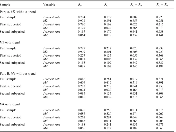
Granger causality tests with respect to nominal GDP. Table

4 reports p-values of Granger causality tests for nominal GDP, where the p-value is the marginal signi® cance level of the predictive value of a particular variable. Part A focuses on theM2aggregate and Part B onM4. Results are given for the whole period and two subperiods where the exact dates of these samples are given in footnotea_{to Table 1. Results}

are presented for estimates with and without the inclusion of a deterministic trend. The results in the table are for a three-variable unrestricted VAR containing a monetary aggre-gate, one interest rate or interest rate spread and nominal GDP, with four lags.9 _{We have also estimated a}

four-vari-able system where, following Friedman and Kuttner (1992) and several other studies, a measure of government expendi-tures is also included. These results are given in Table A.4 of

(7)

Table 3. Johansen’s cointegration tests among4variables: RGDP,Pd, M2or M4, and RC, RC

-

RB, or RL

-

RB(without trend)

RB Full sample 17.9* 10.9 6.0 0.29 35.0 17.2 6.3 0.29 First subperiod 21.1* 10.5 6.4 0.72 38.8 17.7 7.2 0.72 Second subperiod 36.1* 21.7* 17.4* 6.0* 81.3* 45.2* 23.4* 6.0*

1 0_{Alternative speci® cations include tax revenues as an additional variable or use the government de® cit as a ® scal policy measure. These} alternative ® scal policy variables appeared to have little causal e ect on nominal GDP, real GDP or in¯ ation. The government expenditure variable, while its inclusion did not signi® cantly change our conclusions about the predictive value of the ® nancial variables, did in a number of speci® cations have a signi® cant e ect.

1 1_{In Tables 5 and 6 we also do not show p values for the own lags of the variables. Again those are always signi® cant but not of interest.}

the Appendix and do not di er signi® cantly from the results in Table 4.1 0

The numbers in the row marked `interest rate’ refer to each of the four interest rates or spreads, as indicated in the column headings (RB, RC, RC

-

RBand RL

-

RB). The

num-bers in theM2orM4row refer to the marginal signi® cance level of that aggregate in a VAR including the interest rate (or spread) in the respective column. A row giving p-values for the lags of GDP itself is not included because these values are always highly signi® cant ± zero to the three decimal places reported in the table ± and therefore uninfor-mative.

The results in the table have somewhat pessimistic im-plications concerning the usefulness of any of the ® nancial variables we consider as robust information variables or intermediate targets for monetary policy. With either mon-etary aggregate included, the spread between the call money rate and treasury bill rate is informative with respect to GDP, with or without the inclusion of a time trend, in estimates for the whole sample and ® rst-subperiod. This relationship, however, breaks down in the post-1979

sub-period. Depending on the interest rate or interest rate spread and on the time period,M2 andM4 in some cases have predictive value. This is more often the case in esti-mates for separate subperiods than for the whole period. Unlike the Friedman and Kuttner (1992) results for the United States, the money-income relationship, though not particularly robust in Table 4, does not appear to weaken in the post-1979 period.

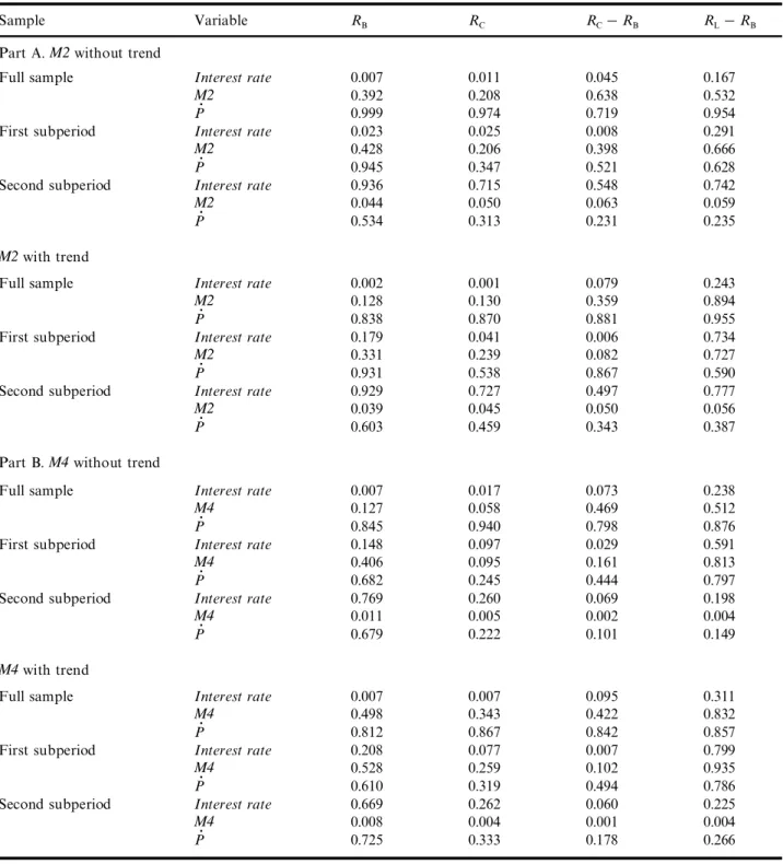
Granger causality tests with respect to real GDP and in¯

a-tion. In Tables 5 and 6 we present results for VARs where

nominal GDP is replaced by real GDP (RGDP) and the in¯ ation rate (Pd). The tables are otherwise parallel to Table 4. Part A again focuses on the M2 aggregate; Part B on

M4.1 1

Real GDP

Table 5 shows a pattern quite di erent from that found by Friedman and Kuttner (1992) and Bernanke and Blinder (1992) for US data. The interest rate, whether measured by

(8)

Table 4. Granger causality tests with respect to nominal GDP(loglevels)

Sample Variable RB RC RC

-

RB RL

-

RB

Part A.M2without trend

Full sample Interest rate 0.794 0.179 0.007 0.923

M2 0.972 0.891 0.753 0.951

First subperiod Interest rate 0.780 0.168 0.027 0.216

M2 0.127 0.022 0.385 0.013

Second subperiod Interest rate 0.197 0.170 0.641 0.938

M2 0.064 0.078 0.332 0.141

M2with trend

M2 0.979 0.801 0.608 0.920

M2 0.001 0.005 0.132 0.065

M2 0.087 0.102 0.345 0.184

Part B.M4without trend

M4 0.606 0.619 0.716 0.891

M4 0.024 0.022 0.466 0.013

M4 0.016 0.039 0.216 0.065

M4with trend

M4 0.687 0.520 0.274 0.909

M4 0.045 0.071 0.568 0.206

M4 0.056 0.122 0.187 0.068

1 2_{Results analogous to those in Tables 5 and 6 for the case where government spending is included as an additional variable are given in} Tables A5 and A6 of the Appendix, available from the authors on request.

the Treasury bill rate or call rate, as well as the call rate-bill rate spread (RC

-

RB) have signi® cant predictive power with

respect to RGDP for the whole period and ® rst subperiod in most speci® cations in the table. This relationship, however, is not present in the second subperiod. The only exception being the call rate± bill rate spread when the M4 is the aggregate. The two monetary aggregates, on the other hand, show little sign of predictive power for the whole period or ® rst subperiod, but are highly signi® cant in the second subperiod. The monetary aggregate (M2orM4) is signi® cant at the 10% level in all 16 speci® cations in the table for the second subperiod and at the 1% level for all eight whereM4

is the aggregate.

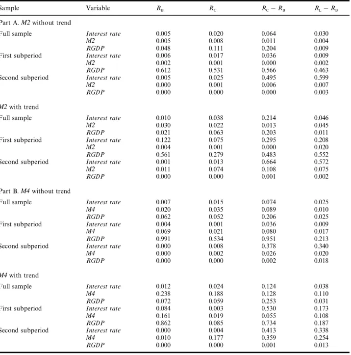
In¯ ation

Table 6 provides results of Granger causality tests with respect to in¯ ation. A very robust relationship is that

tween the interest rate measures, with little to choose be-tween RB and RC, and in¯ ation. This is true for the whole

period and, unlike the result in Tables 4 and 5, for both subperiods. The interest rate spreads are sometimes signi® -cant, but their e ect is less robust, depending on whether a trend is included and on which monetary aggregate is in the VAR.

TheM2aggregate also has robust predictive value with respect to in¯ ation. TheM4aggregate is signi® cant across all time periods, but its signi® cance declines markedly in many speci® cations when a trend is included in the VAR.1 2

Results where the monetary base is the aggregate. As noted

previously, we have also conducted Granger causality tests where money is measured by the monetary base. A di culty for this analysis is that there are several breaks in the quarterly UK series for the base. The longest consistent series available runs from 1963 : 4 to 1986 : 3. This cuts o

(9)

Table 5. Granger causality tests with respect to real GDP (loglevels)

-

RB RL

-

RB

M2 0.392 0.208 0.638 0.532

Pd 0.999 0.974 0.719 0.954

M2 0.428 0.206 0.398 0.666

Pd 0.945 0.347 0.521 0.628

M2 0.044 0.050 0.063 0.059

Pd 0.534 0.313 0.231 0.235

M2with trend

M2 0.128 0.130 0.359 0.894

Pd 0.838 0.870 0.881 0.955

M2 0.331 0.239 0.082 0.727

Pd 0.931 0.538 0.867 0.590

M2 0.039 0.045 0.050 0.056

Pd 0.603 0.459 0.343 0.387

M4 0.127 0.058 0.469 0.512

Pd 0.845 0.940 0.798 0.876

M4 0.406 0.095 0.161 0.813

Pd 0.682 0.245 0.444 0.797

M4 0.011 0.005 0.002 0.004

Pd 0.679 0.222 0.101 0.149

M4with trend

M4 0.498 0.343 0.422 0.832

Pd 0.812 0.867 0.842 0.857

M4 0.528 0.259 0.102 0.935

Pd 0.610 0.319 0.494 0.786

M4 0.008 0.004 0.001 0.004

Pd 0.725 0.333 0.178 0.266

half of the post-1979 period, which is important to our study of the robustness of money± income relationships.

We therefore restrict discussion to the following two comments. (Results from Granger tests using three and four variable VARs analogous to those in Tables 4± 6 are given in Tables A7± A9 of the Appendix.)

1. The base does not have robust predictive power with respect to nominal GDP, real GDP or the in¯ ation rate. This result follows for the whole period and both sub-periods.

2. Inferences about the predictive power of interest rates or interest rate spreads drawn on the basis of VARs where

(10)

Table 6. Granger causality tests with respect to in¯ ation (loglevels)

-

RB RL

-

RB

M2 0.005 0.008 0.011 0.004

RGDP 0.048 0.111 0.204 0.009

M2 0.002 0.001 0.000 0.002

RGDP 0.612 0.531 0.566 0.463

M2 0.000 0.001 0.006 0.007

RGDP 0.000 0.000 0.000 0.003

M2with trend

M2 0.030 0.022 0.013 0.045

RGDP 0.021 0.063 0.203 0.011

M2 0.004 0.001 0.000 0.020

RGDP 0.561 0.279 0.483 0.552

M2 0.011 0.074 0.108 0.075

RGDP 0.000 0.000 0.001 0.002

M4 0.020 0.035 0.089 0.010

RGDP 0.062 0.052 0.206 0.025

M4 0.069 0.021 0.080 0.017

RGDP 0.991 0.534 0.951 0.213

M4 0.000 0.002 0.026 0.020

RGDP 0.000 0.000 0.002 0.018

M4with trend

M4 0.238 0.188 0.128 0.110

RGDP 0.072 0.059 0.253 0.031

M4 0.161 0.019 0.055 0.108

RGDP 0.862 0.085 0.734 0.187

M4 0.010 0.177 0.359 0.254

RGDP 0.000 0.000 0.001 0.013

money is measured by theM2orM4aggregate are not changed substantially when the monetary base is sub-stituted as the monetary aggregate.

Implications of variance decompositions

As explained in Section II, another metric we use to examine the relationship between income and a number of ® nancial variables is a variance decomposition. As noted there, vari-ance decompositions have the advantage that they measure

the predictive power of orthogonalized residuals. They also, of course, have some well-known disadvantage s (see foot note2_).

Tables 7, 8 and 9 show variance decompositions of nom-inal GDP, real GDP and in¯ ation. These variance de-compositions are based on a subset of the VARs used for the Granger tests in Tables 4± 6. The results shown include the

M4aggregate. (Variance decompositions for the same sys-tems using theM2aggregate are shown in Tables A10± A12 of the Appendix, available from authors on request.) The

(11)

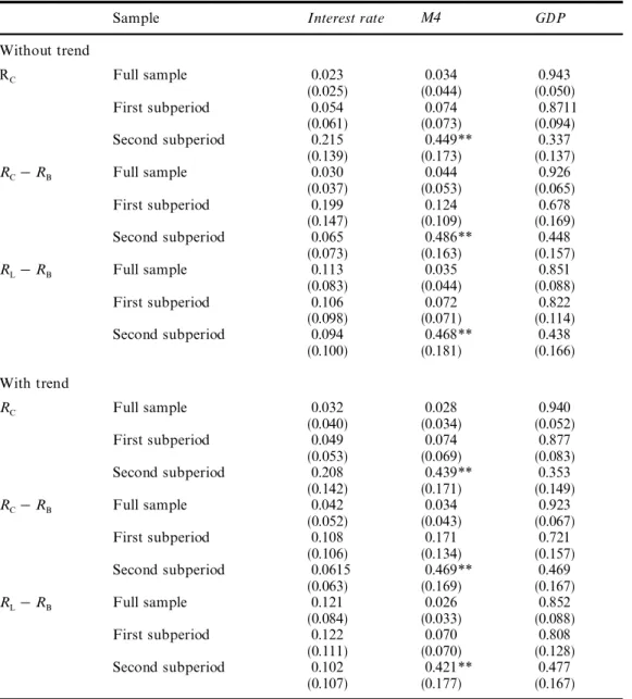
Table 7. Variance decompositions for nominal GDP

Sample Interest rate M4 GDP

Without trend RC Full sample 0.023 0.034 0.943 (0.025) (0.044) (0.050) First subperiod 0.054 0.074 0.8711 (0.061) (0.073) (0.094) Second subperiod 0.215 0.449** 0.337 (0.139) (0.173) (0.137) RC

-

RB Full sample 0.030 0.044 0.926 (0.037) (0.053) (0.065) First subperiod 0.199 0.124 0.678 (0.147) (0.109) (0.169) Second subperiod 0.065 0.486** 0.448 (0.073) (0.163) (0.157) RL

-

(12)

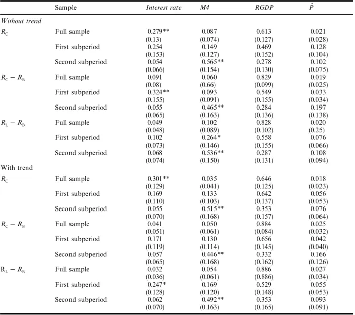
Table 8. Variance decompositions for real GDP

Sample Interest rate M4 RGDP Pd

Without trend RC Full sample 0.279** 0.087 0.613 0.021 (0.13) (0.074) (0.127) (0.028) First subperiod 0.254 0.149 0.469 0.128 (0.153) (0.127) (0.152) (0.104) Second subperiod 0.054 0.565** 0.278 0.102 (0.066) (0.154) (0.130) (0.075) RC

-

RB Full sample 0.091 0.060 0.829 0.019 (0.08) (0.66) (0.099) (0.025) First subperiod 0.324** 0.093 0.549 0.033 (0.155) (0.091) (0.155) (0.034) Second subperiod 0.055 0.465** 0.284 0.197 (0.065) (0.163) (0.136) (0.138) RL

-

RB Full sample 0.049 0.102 0.828 0.020 (0.048) (0.089) (0.102) (0.25) First subperiod 0.102 0.264* 0.558 0.076 (0.073) (0.146) (0.155) (0.066) Second subperiod 0.068 0.536** 0.287 0.108 (0.074) (0.150) (0.131) (0.094) With trend RC Full sample 0.301** 0.035 0.646 0.018 (0.129) (0.041) (0.125) (0.023) First subperiod 0.169 0.133 0.642 0.056 (0.110) (0.103) (0.137) (0.053) Second subperiod 0.055 0.515** 0.353 0.076 (0.070) (0.168) (0.157) (0.064) RC

-

RB Full sample 0.041 0.050 0.884 0.025 (0.051) (0.061) (0.084) (0.032) First subperiod 0.171 0.130 0.656 0.042 (0.119) (0.114) (0.145) (0.040) Second subperiod 0.057 0.446** 0.332 0.166 (0.065) (0.168) (0.162) (0.126) RL

-

RB Full sample 0.032 0.054 0.886 0.027 (0.036) (0.061) (0.886) (0.034) First subperiod 0.247* 0.169 0.529 0.055 (0.128) (0.120) (0.148) (0.053) Second subperiod 0.062 0.492** 0.353 0.093 (0.070) (0.163) (0.165) (0.091)

**Indicates signi® cance at 5% level. Stars are shown only for money and interest rate variables not for income or in¯ ation.

1 3_{The same holds true for the M2 aggregate.}

1 4_{The M2 aggregate is signi® cant in all 18 speci® cations.}

interest rate spreads included explains a statistically signi® -cant portion of GDP forecast variance for the whole period or either subperiod.

Real GDP. In Table 8, the most striking result is that the

M4aggregate explains a large fraction of the forecast vari-ance of real GDP, in the second subperiod. Again this result is statistically signi® cant at the 5% level in all speci® ca-tions.1 3 _{In some speci® cations an interest rate (or interest}

rate spread) measure explains a statistically signi® cant por-tion of real GDP variance, but in each case this is for the whole period or ® rst subperiod.

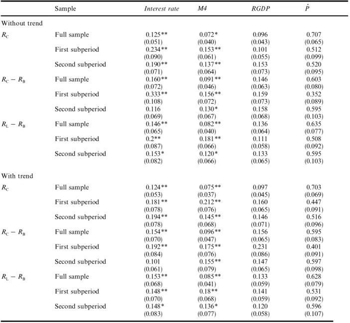
In¯ ation. From the results in Table 9, it can be seen that

both the M4 aggregate and each interest rate (or spread) measure explain a signi® cant fraction of the forecast vari-ance of in¯ ation. The interest rate measure typically ex-plains between 10 and 20% of the forecast variance of in¯ ation and is signi® cant at the 10% level in 16 of 18 speci® cations (at the 5% level in 14) in the table.M4explains anywhere from 7± 8% to 18± 20% of the forecast variance of in¯ ation and is signi® cant at the 10% level in all 18 speci-® cations (at the 5% level in 14).1 4

Both interest rate measures and the monetary aggregate appear to have a robust relationship with the in¯ ation rate

(13)

Table 9. Variance decompositions for in¯ ation

Sample Interest rate M4 RGDP Pd

Without trend RC Full sample 0.125** 0.072* 0.096 0.707 (0.051) (0.040) (0.043) (0.065) First subperiod 0.234** 0.153** 0.101 0.512 (0.090) (0.061) (0.055) (0.099) Second subperiod 0.190** 0.137** 0.153 0.520 (0.071) (0.064) (0.073) (0.095) RC

-

RB Full sample 0.160** 0.091** 0.146 0.603 (0.072) (0.046) (0.063) (0.080) First subperiod 0.333** 0.156** 0.159 0.352 (0.108) (0.072) (0.073) (0.089) Second subperiod 0.116 0.130* 0.158 0.595 (0.069) (0.067) (0.068) (0.103) RL

-

RB Full sample 0.146** 0.082** 0.136 0.635 (0.065) (0.040) (0.064) (0.077) First subperiod 0.2** 0.181** 0.111 0.508 (0.087) (0.066) (0.058) (0.092) Second subperiod 0.153* 0.120* 0.133 0.595 (0.082) (0.066) (0.065) (0.103) With trend RC Full sample 0.124** 0.075** 0.097 0.703 (0.053) (0.037) (0.045) (0.069) First subperiod 0.181** 0.212** 0.160 0.447 (0.078) (0.076) (0.065) (0.091) Second subperiod 0.194** 0.145** 0.146 0.516 (0.078) (0.068) (0.071) (0.096) RC

-

RB Full sample 0.154** 0.096** 0.156 0.595 (0.070) (0.047) (0.065) (0.083) First subperiod 0.192** 0.175** 0.231 0.401 (0.084) (0.076) (0.086) (0.091) Second subperiod 0.101 0.155** 0.147 0.597 (0.061) (0.079) (0.065) (0.098) RL

-

RB Full sample 0.153** 0.085** 0.133 0.628 (0.068) (0.041) (0.059) (0.079) First subperiod 0.148** 0.18** 0.141 0.531 (0.070) (0.068) (0.059) (0.092) Second subperiod 0.148* 0.136* 0.120 0.596 (0.083) (0.077) (0.058) (0.107)

**Indicates signi® cance at 5% level. Stars are shown only for money and interest rate variables not for income and in¯ ation.

as measured by the metric of variance decompositions, for the whole period and both subperiods.

IV . S UM M ARY AN D PO LI CY I M PLICATI ONS

Summary

We have examined the relationship between a number of ® nancial variables and traditional monetary policy goals. With respect to nominal GDP, our variance

decomposi-tions suggest that a monetary aggregate (M2orM4) would be a good information variable (or intermediate target) based on evidence from the post-1979 period. We do not, however, ® nd strong evidence of a Granger causal relation-ship for either monetary aggregate for this subperiod.

Results for real GDP and the in¯ ation rate are more robust. For real GDP in the post-1979 period, both the results of Granger tests and variance decompositions suggest that both monetary aggregates (M2 and M4) are good information (or intermediate target) variables. Here, our United Kingdom results are in contrast to Friedman and Kuttner’s (1992) results for the United States which

(14)

1 5_{The variance decompositions shown in the text are only for the call rate (R}

C). Results substituting the treasury bill rate (RB) produce very similar results.

1 6_{For simplicity, the ® gures do not show con® dence intervals. Computed con® dence intervals for these impulse response functions indicate} that the responses of GDP and RGDP are signi® cantly di erent from zero for 12 and 6 quarters, respectively.

show a breakdown in the money-income relationship in the 1980s.

Because UK monetary policy has followed a strategy of targeting in¯ ation in the period since 1992, our in¯ ation results are perhaps of most interest. There is a robust rela-tionship between in¯ ation and both interest rates (RB, RC)

that we considered. The interest rate measures are strongly Granger causal and explain a signi® cant fraction of the forecast variance of in¯ ation.1 5 _{These results are robust}

across the subperiods we consider. Interest rate spreads are also signi® cant in variance decompositions, but there is less evidence that they are Granger causal with respect to in¯ a-tion.

Both monetary aggregates are signi® cant in variance de-compositions in the post-1979 subperiod. Granger causality tests also show a signi® cant relationship between M2 and in¯ ation in this subperiod, as well as in the earlier one. Evidence of Granger causality from M4to in¯ ation is less clear ± its signi® cance depending on whether or not a trend is included in the VAR.

Policy implications

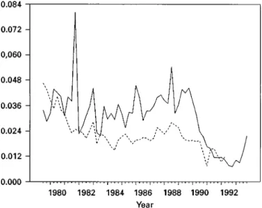
The ® nding that broader monetary aggregates are informa-tive with respect to monetary policy goal variables in the post-1979 period is at odds with the conventional view; which view holds that broad aggregates have been unreli-able predictors of both nominal and real GDP since 1979. This discrepancy suggests the usefulness of further examina-tion of the money- income relaexamina-tionship during these years. Figures 1 and 2 show plots of the growth rates inM4and, respectively, nominal and real GDP. While statements about such graphs are necessarily imprecise, it appears to us that instability in the money± income relationship is most apparent in the early 1980s. From the mid-1980s the series have many periods of positive co-movement. It appears a possibility, therefore, that the conventional view is based on the experience of the early 1980s. Figures 3 and 4 plot impulse response functions to a shock to M4. The ® gures show substantial positive responses of both nominal and real GNP to innovations in M4(all variables measured in natural logs). Figure 4, however, does not indicate a signi® -cant response of in¯ ation to innovations inM4.1 6

The plots in Figs 1± 4 are on the whole supportive of the view that monetary aggregates have been informative with respect to monetary goal variables in the post-1979 period

± an essential quali® cation for a ® nancial variable to be

a useful information variable.

As explained in Section II, however, a ® nancial variable may be informative without being truly causal, or structural,

Fig. 1. M4 (Ð Ð ) and GDP (- - - -) growth rates for the second

subperiod

Fig. 2. M4 (Ð Ð ) and RGDP (- - - -) growth rates for the second

subperiods

in the sense of Bernanke (1993). If the ® nancial variable is chosen as an intermediate target a relationship with the policy goal variable, due for example to reverse causation or mutual causation from some other variable, may break-down. To examine further the nature of the relationship between income and monetary aggregates, we consider Granger tests of the e ect of GDP onM2andM4. Table 10

(15)

1 7_{The interest rate included in these VARS is the call rate (R} C). 1 8_{Mutual causation from some other variable(s) is also possible.} Fig. 3. Responses to M4: call rate (Ð Ð ), M4(...) and GDP (- - - -)

Fig. 4. Responses to M4: call rate (Ð Ð ),M4(...), Real GDP ( ± ´± ´), in¯ ation (± ´´± ´´± )

shows marginal signi® cance levels (p-values) for the e ects GDP onM2andM4in the same estimated VARS for which results are shown in Table 4.1 7 _{Results are for the second}

subperiod. GDP is seen to have signi® cant predictive power with respect to both monetary aggregates. Figure 5 shows an impulse response function for the e ect on M4 of an innovation to GDP. M4shows a strong positive response again consistent with causality from GDP to money.

Our results in this section indicate that the money± in-come relationship is one of feedback, rather than of one-directional causality from money to income.1 8 _{If this is the}

Fig. 5. Responses to GDP: call rate (Ð Ð ),M4(...),GDP(- - - -)

Table 10. Marginal signi® cance levels (p-values): Granger causality

from GDP to monetary aggregates

M2 M4

With trend 0.050 0.004

Without trend 0.037 0.005

case our overall results are more supportive of a role for a monetary aggregate as an information variable rather than an intermediate target.

V. CON CLUS ION

Our results were summarized in the previous section. Here we have only a concluding comment.

Friedman (1993, p. 182) argues that `once the policymak-ing procedure is framed in terms of information variables, rather than an intermediate target, there is no reason why interest rate relationships are any less suitable for this pur-pose than monetary aggregates.’ Our results indicate that for the United Kingdom interest rates are informative with respect to monetary policy goals. Our results also indicate that broad monetary aggregates are also potentially useful as information variables.

RE FERE NC ES

Bernanke, B. S. (1993) How important is the credit channel in the transmission of monetary policy?: A comment, Carneg

ie-Rochester Conference Series on Public Policy,39, 47± 52.

(16)

Bernanke, B. S. and Blinder, A. S. (1992) The Federal funds rate and the channels of monetary transmission, American Eco-nomic Review,82, 901± 21.

Chrystal, K. A. and McDonald, R. (1994) Empirical evidence on the recent behavior and usefulness of simple-sum and weighted measures of the money stock, Federal Reserve Bank of St.Louis Review,76, 73± 109.

Engle, R. A. and Granger, C. W. J. (1987) Cointegration and error correction: Representation, estimation, and testing, Econo-metrica,55, 251± 76.

Feldstein, M. and Stock, J. H. (1994) The use of a monetary aggregate to target nominal GDP, in N. G. Mankiw (ed.) Monetary Policy, University of Chicago Press, Chicago, IL. Friedman, B. M. (1993) The role of judgment and discretion in the

conduct of monetary policy, in Changing Capital Markets:

Implications for Monetary Policy, Federal Reserve Bank of Kansas City.

Friedman, B. M. and Kuttner, K. N. (1992) Money, income, and interest rates, American Economic Review,82, 472± 92. Friedman, B. M. and Kuttner, K. N. (1993) Another look at the

evidence on money-income causality, Journal of Econometrics,

57, 189± 203.

Friedman, B. M. and Schwartz, A. (1982) MonetaryTrends in the United States and theUnited Kingdom, University of Chicago Press, Chicago, IL.

Harvey, A. (1990)The Econometric Analysis ofTime Series, Philip Allan, Oxford.

Hansen, H. and Juselius, K. (1995) Cats in Rats Cointegration

Analysis ofTime Series, Estina, Evanston, IL.

Johansen, S. (1991) Estimation and hypothesis testing of cointeg-rating vectors in Gaussian vector autoregressive models, Econometrica,59, 1551± 80.

Johansen, S. and Juselius, K. (1992) Maximum likelihood estima-tion and inference on cointegraestima-tion-with applicaestima-tion to the demand for money, Oxford Bulletin of Economics and Statis-tics,52, 169± 209.

King, R. G., Plosser, C.I., Stock, J. H. and Watson, M. W. (1991) Stochastic trends and economic ¯ uctuations, American Eco-nomic Review,81, 819± 40.

Moersch, M. (1996) On the predictive power of interest rate spreads for output, Journal of Economics and Business, 48, 185± 99.

Phillips, P. C. B. and Ouliars, S. (1990) Asymptotic properties of residual based tests for cointegration, Econometrica, 58, 165± 93.

Phillips, P. C. B. and Perron, P. (1988) Testing for a unit root in time series regression, Biometrika,75, 335± 46.

Ramey, V. (1993) How important is the credit channel in the transmission of momentary policy?, Carnegie-Rochester

Con-ference Series on Public Policy,39, 1± 45.

Sims, C. A. (1992) Interpreting the macroeconomic time series facts, European Economic Review,36, 975± 1011.

Sims, C. A., Stock, J. H. and Watson, M. W. (1990) Inference in linear systems time series models with some unit roots, Econo-metrica,58,113± 44.

Stock, J. H. and Watson, M. W. (1988) Testing for common trends, Journal of the American Statistical Association, 83, 1097± 107.

Stock, J. H. and Watson, M. W. (1989) Interpreting the evidence on money-income causality, Journal of Econometrics, 40, 161± 81.

Stock, J. H. and Watson, M. W. (1993) A simple estimator of cointegrating vectors in higher order integrated systems, Econometrica,61, 783± 920.