rs
/S 6
.
s
GENERATING A ROBUST MODEL FOR
PRODUCTION AND INVENTORY CONTRO!
41 X* ^
SUS^^ITTED TO ThiE DEP
aRT..-.E..7
. a i. £<y 0 w T R J
jT» .
S H G iN E E R lN Q
^0 THE i HS Tl T^TE 0 ? EMGiHE
«— i « 4 Lm ^•T 1
!.N PAHTiiAL
GENERATING A ROBUST MODEL FOR
PRODUCTION AND INVENTORY CONTROL
A THESIS
SUBMITTED TO THE DEPARTMENT OF INDUSTRIAL
ENGINEERING
AND THE INSTITUTE OF ENGINEERING AND SCIENCES
OF BILKENT UNIVERSITY
IN PARTIAL FULFILLMENT OF THE REQUIREMENTS
FOR THE DEGREE OF MASTER OF SCIENCE
By
Asli Sencer
Februarv. 1993
TS
1 5 6
11
I certify th at I have read this thesis and that in my opinion it is fully adequate, in scope and in quality, as a thesis for the degree of Master of Science.
Professor Doctor líWirn Doğrusöz(Principal A ^ m s ^
I certiiy tluit I h¿ıve rc^id this thesis and that in my opinion it is fully ¿idecjuate in sco[)c and in quality, as a thesis tor tlie degree of Master of Scieuice.
Associate^ Professor Doctor Oiner Ihr
I cer tiiy t h a t 1 luive rea,d this thesis and t h a t in my opi ni on it is ivdly adecpiate, in sc(.)pc a n d in quality, as a tlursis for the degree of Mast(n· of Science.
AssociatWi^ToTes^o Cemal Dinçer
I certify t h a t I have rcc'ul this tlursis and t h a t in m\' opi ni on it is full}' adt'Cjuatc' in scope' aiu;l in cjualilw a.s a thesis for tlu' i:l(ugr(‘(' of M a s t e r c;f Scicuu'e.
о
Associate Professor Doctor Erdal Erel
I certify that I have read tliis thesis and that in my opinion it is fully adequate in scope and in quality, as a thesis for the degree of Master of Science.
Associate Professor Doctor Barbaros Tansel
Approved for the Institute of Engineering and Sciences:
M U l
Professor Doctor Mehirtet Baray
ABSTRACT
GENERATING A ROBUST MODEL FOR PRODUGTION
AND INVENTORY GONTROL
Aslı Sencer
M.S. in Industrial Engineering
Supervisor; Professor Doctor Halim Doğrusöz
February, 1993
In tills stud}', we generate a production and inventory control model which gives h'obust‘ solutions against demand estimation errors. This model is applied to a real production and inventory system; howe\’er, it is a general model where the demand rate is stochastic with a known probability distribution and other parameters of the system are constant. The proposed model is a bi-objective chicision making model, with two decision variables. .A ‘compromised* solution is found for the problem using the trade-off curve generated by a constrained sequential optimization technique, applied on a nonlinear programming model parametrically. Robustness against parameter estimation errors is tested by sensitivity analysis. Here a new dimension is added to sensitivity analysis methodology by including a sensitivity measure as a ‘cost of error* of parameter estimation. By so doing, the proposed model is tested against the classical EOQ model and it is shown that the proposed model ])erforms far better.
Key words: Production and Inventory Control, Economic Order Quantity,
.Sensitivity Analysis, Robustness, Cost of Error.
ÖZET
PARAMETRE TAHMİNİNDEKİ HATALARA DAYANIKLI
BİR ÜRETİM VE ENVANTER KONTROL MODELİ
Aslı Sencer
Endüstri Mühendisliği Bölümü Yüksek Lisans
Tez Yöneticisi: Prof. Dr. Halim Doğrusöz
Şubat, 1993
Bu çalışmada, talep tahminindeki hatalara karşı dayanıklı çözümler üreten bir ürctim-stok kontrol modeli geliştirilmiştir. Bu model, gcı çek bir üretim-stok kontrol sistemine uygulanmak üzere kurulmuştur. Önerilen model, çift amaçlı ve iki karar değişkenli bir karar modeli olup, talebin, yoğunluk fonksiyonu bi linen bir rastlantı değişkeni ve diğer parametrelerin sabit olduğu varsayımına dayanmaktadır. Modelde öngörülen 1-Maliyet minimizasyonu ve 2-Karşılanan talep yüzdesi maksimizasyonu amaçları arasında bir uzlaşık çözüm elde et meye bciz olacak bir değiş-tokuş eğrisi, modeli tek kısıtlı bir matematik pro gramlama modeli gibi ve parametrik olarak işleterek elde edilmektedir. Mode lin ve modelden elde edilen çözümün parametre tahminlerindeki hatalara karşı dayanıklılığı (robustness) duyarlık analizi ile ölçülüyor. Burada duyarlık ölçüsü olarak parametre tahminlerindeki ’hatanın m aliyeti’ kullanılmakla, duyarlık analizi metodolojisine yeni bir boyut getirilmektedir. Böylelikle, önerilen model, klasik BOQ (ekonomik sipariş miktarı) modeliyle karşılaştırılmakta ve EOQ modeline göre daha iyi .sonuç verdiği gösterilmektedir.
Anahtar sözcükler. Üretim ve Stok Kontrolü, Ekonomik Sipariş Miktarı,
Duyarlık Analizi, Dayanıklılık, Hata Maliyeti.
/ACKNOWLEDGEMENT
r\
I am indobted to Professor Doctor Halim l.)o,y;rıısöz for his sup(.'r\'isi(;n, and sui2:c;ostions throiiiHioiit this thesis stiidw I am e^rateful to Associate Prcd'essor Doctor Omcr Benli and Associate Professor Doctor Barbaros Tansel for their valuable guidance and comments. I am thankful to Associate Professor Doctor Cemal Dinçer and Associate Professor Doctor Elrdal Erel for their interest in my thesis.
I would lik(' to exti'iid m\' deepest giatitinh' and thanks to my fanniv ainl to my liance lor rheir nioi'ale sup|)ort and enroura-genKuit, e.speciall}· at tinu's of despair and hardship. It is to them this study is dedicated, without whom it would not have been possible.
I really wish to express my sincere thanks to Levent Kandiller whose pre cious friendship, guidance and support turned my times of despair into enjoy able moments. I want to express my gratitude to Vedat Verter and Ceyda Oğuz for helping me with in any kind of computer work. And the last but not the least, I am grateful to rny classmates Ihsan Durusoy, Hakan Ozakta.ş and to my officemates Gillcan Yeşilkokçen, Mehmet Özkan, Pınar Keskinocak and Sibel Salman who shared rny enthusiasnr during the entire period of M.S. studies.
C ontents
1 IN T R O D U C T IO N 1
2 LITERATURE REVIEW 6
3 PRODUCTION AND INVENTORY CONTROL PROBLEM
UNDER CONSIDERATION 13
3.1 SYSTEiVI ANALYSIS 13
3.2 OB.JECTIVES 22
4 MODEL CONSTRUCTION 30
4.1 REVIEW OF CLASSICAL EOQ M O D E L ... 34
4.2 DERIVATION OF THE SPIL MODEL 37
4.3 SOLUTION T EC H N IQ U E ... 44
5 SENSITIVITY ANALYSIS ON THE EOQ AND SPIL MOD
ELS TO FACILITATE LEARNING 49
5.1 SENSITIVITY OF THE OPTIMUM SOLUTION Q* OR U TO
THE CHANGES IN P A R A M E T E R S ... 52
CONTENTS VHl
5.1.1 Sensitivity of the optimal solution to the changes in D: . 52
5.1.2 Sensitivity of the optimal solution to the changes in r: 53
5.1.3 Sensitivity of the optimal solution to the changes in S and h : ... 54
5.2 CH.ANGE IN THE TOTAL COST FUNCTION WHEN Q OR / IS N O N O P T IM A L ... 55
5.3 COST OF AN ESTIMATION E R R O R ... 57
5.3.1 Cost of an Estimcition Error in Demand Rate 57
5.3.2 Cost of an Error in Estimating the Other Param eters of
the System 72
List of F igures
3.1 Relations between the system of objectives under consideration . 25
4.1 Change in the inventory level when the S P I L model is applied. 31
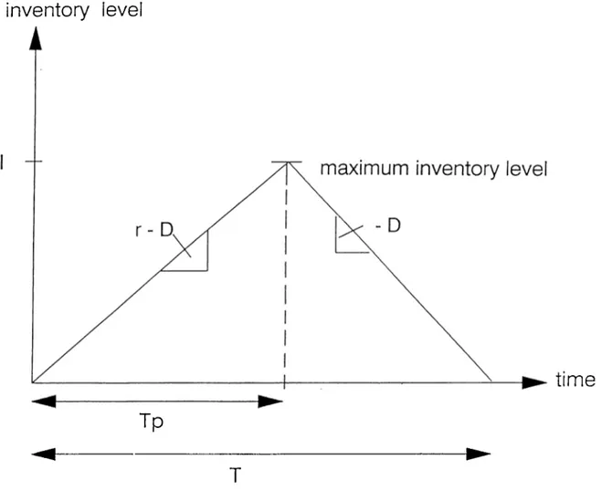
4.2 Change in the inventory level of the classical EOQ model with
fixed production r a t e ... 37
4.3 B{g) versus g ( a = 0 .8 0 ) ... 46
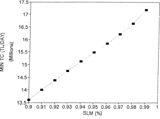
4.4 Total cost function versus / (o;= 0.95)... 47
4.5 The trade-off curve showing the min total cost versus a ... 48
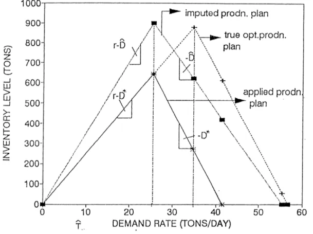
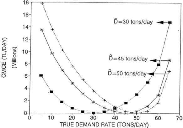
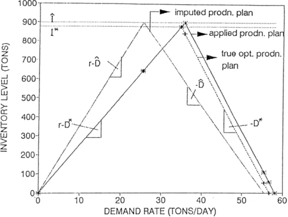
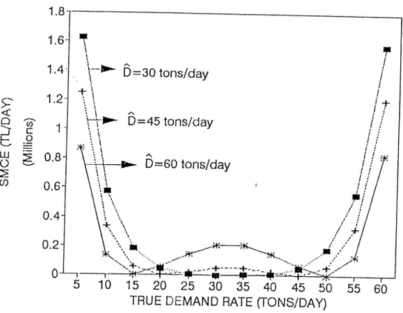
5.1 Change in the production plan due to an error in estimating D, when the decision variable is Q 58 5.2 C M C F versus true demand rate (77’·) 61 5.3 Change in the production plan due to an error in estimating D, when the decision variable is I 62 5.4 S M C E versus true demand rate {D '')... 65
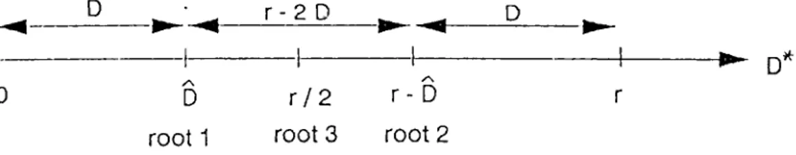
5.5 Roots of the Cost of Error function in S P I L m o d e l ... 67
5.6 Comparison of the cost of a demand rate estimation error in the classical EOQ model and the S P I L m o d e l... 68
LIST OF FIGURES
5.7 Difference of ‘the cost associated due to a demand rate estima
tion error‘ in the classical EOQ and S P I L model versus the true demand I'ate, (i.e, C M C E — S M C E versus D * ) ...
5.8
69
Ratio of the cost of a demand rate estimation error versus the % error in demand rate estimation in the classical EOQ and S P I L
model. 71
5.9 Cost of an error due to a set-up cost estimation error vs the true value of set-up cost (,?*) in the classical EOQ model and SP IL·
model 74
5.10 Cost of an error due to a unit inventory holding cost estimation error vs the true value of unit inventory holding cost (/i*) in the classical EOQ model and S P I L m o d e l ... 76
5.11 Cost of an error due to a production rate estimation error vs the true value of production rate (?■*) in the classical EOQ model and S P I L m o d e l ... 78
List of Tables
4.1 Optimum solution of the S P I L model for different values of o . 48
C hapter 1
IN T R O D U C T IO N
Developing models for controlling production and inventory systems has been a major area for many researchers since the beginning of this century. As defined by Hax and Candea [14], production and inventory systems are concerned with the effective management of the total flow of goods from the acquisition of raw materials to the delivery of finished goods to the final customer.
In this thesis, we try to generate a production and inventory control model which gives insensitive solutions against demand estimation errors. The inspi ration for this thesis subject came from a project conducted for production and inventory control in a process industry, a state enterprise PETKIM. Here, our aim is to design a control system which can be applied to this real system and used in the long run.
Very briefly, the problem of a plant manager in PETKIM is a specific pro duction and inventory control problem. PETKIM is a huge complex with several factories; recently most of the managers are faced with the problem of increasing inventory levels and they can not cope with the financial burden of those inventory. What they need is a control system that provides an effec tive management of the elements (stocks, products, working staff, etc.,) of the system in order to deliver the final products in appropriate quantities, at the desired time, quality and at a reasonable cost.
In fact the aforementioned problem can be solved by using a general pro duction and inventory control model; however when we look over the literature, we can see that most of the theoretical production and inventory control mod els were either misunderstood or not accepted by the managers in the past. The essence of implementation -especially for cases, th at propose a change in ways of thinking- is to achieve wser acceptance and comfort. No m atter how a powerful system is created, it will be useless unless it is well understood and appreciated by the decision maker (DM). T h a t’s why in this thesis we will start by developing an in\'entory control model which will enable the DM to understand the benefits of the decision system, the decisions that are being made and results of those decisions in terms of the meaningful performance measures. This subject is analyzed by many researchers in the literature and are discussed in the next chapter [15] [19] [2.3] [26].
In this thesis we try to design a control system which has the basic prop erties discussed in the following paragraphs. Accordingl}', a production and inventory control system should primarily
• Guide the decision maker to decide.
DM is the person who controls the production and inventory system. He needs an assistance while deciding on when, at what rate and how much to produce, etc. to achieve a certain service level. In this thesis, our aim is to develop a system which will give that assistance to the DM. By ’assistance’, we mean that the DM should not be kept out of the decision process; quite the con trary, he should actively be involved in the decision process, rather than being rejjlaced by an inventory control model. Thus, we should design a production and inventory control system that will generate solutions that incorporate the intuition of the DM.
CHAPTER 1. INTRODUCTION 2
The reason for searching for an information system-rather than a mathe matical optimization model- is derived from the observation that,a m athem at ical model is only an approximation of the real world. An optimization model is characterized by the decision variables that optimize a well-defined goal (i.e..
objective function) with respect to a set of constraints. The optimum solution of the model provides the ’best’ vector of decisions, which means any other solution will be inferior to that of the optimum provided that the model is a ’perfect’ representation of the real system. However, we know that these models involve a lot of initial assumptions and estimates. Thus any change in the initial estimates of the parameters of the model for instance may lead to incorrect decisions. The DM should be able to explain the reasons of the deviations from the expected outcome. In other words, he should be able to control the system by guessing what inputs provide what outputs and what are effects of a change. In this sense, a production and inventory control model should provide an effective assistance for the DM to help him /her learn the production system. Then we should, state that another im portant property of our system is to
• Assist DM to learn how the system works.
As we have discussed in the above paragraphs, if a change occurs in the initial assumptions made, inventory control models may lead to misleading solutions. As we have repeated earlier, in this thesis our aim is to generate a model that gives insensitive solutions to changes in the initial estimates of the input parameters. Thus the model itself gives adaptive decisions while assisting the DM. We define these models as robust inventory control models and introduce a concept as the robxistness of a model. This property is analyzed in detail in the next chapters. Thus another significant property of our model is to
• Generate adaptive decisions due to changes in the initial estimates of the parameters.
CHAPTER 1. INTRODUCTION 3
Our model is a bi-objective decision making model with two decision vari ables. We try to build up a control mechanism which enables the DM to make a trade-off between two conflicting objectives of minimizing the total cost (set-up cost and the inventory holding cost) and maximizing the service level, which is measured in terms of the ratio of the customers satisfied on time. The model
generates a control mechanism similar to that of (s,S) policy type inventory control models. Thus, the decision variables are the maximum inventory level (produce up to level) and the reorder inventory level.
Our model originates from the classical EOQ model with a finite produc tion rate. We know that EOQ model is based on the ‘constant‘ demand rate assumption. When the demand rate is stochastic with a known distribution, it is likely that the solution is in error due to random fluctuations. In literature, it is shown that the optimal solution of EOQ model is insensitive to parameter estimation errors in demand rate. However, we now show that the cost, associ
ated with a demand estimation error may be significantly large in EOQ model
when the demands are stochastic. Thus we modify the classical EOQ model by changing the decision variable from the production quantity Q to maximum inventory level / and show that this new model is insensitive to dejiiand esti mation errors when compared to the classical EOQ model. Using this model, we generate a reorder level model by incorporating the decisions related to the choice of the reorder level into the model. Thi.s optimization model is used to find the optimum values of the reorder level and maximum inventory level that minimizes the total cost function and provide a service level whose lower bound is defined by the DM. Thus our model generates an interactive control mechanism in which the intuition of the DM is activelv involved.
CHAPTER 1. INTRODUCTION 4
In the next chapters, we try to explain our methodology while generating a robust and adaptive decision making model that will assist the DM while giving production and inventory control decisions. In chapter 2, we give a brief literature review of the inventory control models and then state the literature related to the difficulties encountered in iniplementing the theoretical models. In chapter 3, we define the properties of our production and inventory con trol system and discuss the main elements of our system of objectives that are considered in thesis work. Then in chapter 4, we state the steps followed in constructing the production and inventory control model. Chapter 5 includes the sensitivity analysis of our generated model to the estimation errors in the input parameters of the model and also includes the comparison of the perfor mance of this model to that of the classical EOQ model. In chapter 6, we state
CHAPTER 1. INTRODUCTION
C hapter 2
L IT E R A T U R E R E V IE W
The earliest known analysis of inventory systems is made by Ford W hitman Harris, who first presented the ‘economic order quantity‘ EOQ model in a publication in 1913 [13]. Harris‘s basic EOQ model became a paradigm for order quantity analysis, for at least the next 30 years. During this period, much confusion developed over Hie origin of the EOQ model. Most people know the EOQ formula as the Wilson''^, lot size formula -as R.H.Wilson is claimed to be the first to use this formula in practice- while the others know it as Greenes formula and until thirties, for many Europeans it had been known as Ca7ii]/s formula. Although the original article may have been unknown for many years, the chapter version has been cited since 1931. In 1931, Raymond F.E. (see [11] for reference) gave Harris as the source of the EOQ formula; but the confusion about the formula‘s origin has persisted until its rediscovery in 1988 by Erlenkotter [10] [11].
During this period, the original EOQ model is developed by Taft (1918) (see [11] for reference) and used by many others like Green, Wilson , Alford, etc. Taft and Cooper analyzed a production and inventory system in which the production rate was finite. In 1928, Thornton C. Eiw introduced the probability theory into the inventory models. He studied the cases where the demand rate is not known precisely.
Interest in the study of inventory systems has increased since World War II and numerous publications have been devoted solely to this subject. Wagner
and Whiiin [27] published an extension of the EOQ model in 1958 in which
time phased dynamic demand and infinite production capacity over a finite planning horizon is considered.
With the advance of the mathematical inventory theory and easy availabil ity of cheaper computer time, many researchers started to work on different types of inventory control models. Actually, the classical EOQ models have too many ‘static‘ assumptions like ‘constant' demand rate, constant production rate and lead time, etc. and therefore designated as a static model. However in the world these static assumptions hardly ever hold. Aggarwall [4] divides the inventory systems into two main categories in his ‘review of current inventory theory and applications' paper (1974);
• Static inventory control models
• Dynamic inventory control models.
Dynamic models, which require a considerable amount of computation effort are obtained by varying ’constant' assumption for one or more of the variables of the static model. Other classification schemes are provided by Silver [23] and Nahrnias [21]; but they all agree on such basic classifications. Dynamic models are stochastic if there is randomness in the process; otherwise they are
deterministic. Thus we introduce a sub-classification:
• Stochastic vs. Deterministic dynamic inventory control models
These classifications can be further developed by considering the following properties of the inventory models;
CHAPTER 2. LITERATURE REVIEW 7
• Single vs. Multiple items
CHAPTER 2. LITERATURE REVIEW
• Backorders vs. Lost sales
• Zero vs Constant vs Random lead times
• Finite vs. Infinite planning horizon
• Various types of constraints and others.
More complex inventory systems are formed with several combinations of the above properties. We may give some well known examples from the literature: In 1971, Lasdon and Terjung investigated the multi-item inventory systems. In seventies, Zangwill [4] among others considered linking together of several single facilities and multiple products. Zangwill analyzed a deterministic multi period production and inventory model that had concave production costs with backlogging allowed. Porteus [22] considered single product, periodic review, stochastic inventory model with concave cost function. Next, he advanced his previous results to prove that a generalized (s,S) policy would be optimal in a finite horizon problem, where demands were uniform.
While the deterministic inventory models were being developed by many other researchers, several others started working on stochastic inventory mod els. Apparently, when the parameter values vary stochastically with time, we can no longer assume that the best strategy is the one obtained from the de terministic model. This prevents us from using simple average costs over a finite or infinite planning horizon as was possible in EOQ derivation. Instead, we now have to use the information on the random parameter over a finite period, extending from the present when determining the appropriate value of current replenishment quantity. Another element of the problem that is im portant in selecting appropriate replenishment quantities is whether replen ishments should be scheduled at specified discrete points in time or whether they can be scheduled at any point in continuous time. Thus the stochastic inventory control models can be •
CHAPTER 2. LITERATURE REVIEW
Still another factor that can materially influence the logic in selecting replen ishment quantities is the information about the distribution of the random variable. In this thesis we specifically deal with models where the demand is random with a known distribution. We try to develop a production and in ventory control model which allow for variations of the demand rate and still assure a proper control of the inventory levels. In the literature we encounter three basic types of stochastic inventory models:
A frequently used control procedure in practice is what is called an (s,Q) or two-bin system: it involves continuous review, a fixed reorder level (s) and fixed order quantity (Q). Decision rules have been developed for finding Q and s for a wide of choice of shortage costing methods and types of service constraints.
Another common control system is an (R,.S) or periodic replenishment sys tem in which an order is placed every R units of time sufficient to raise the inventory position to an order-up-to level S. .Although the physical operation and costs of (R..S) and (s,Q) systems are likely to be quite different, it can be shown that the determination of S in (R,S) system is equivalent mathematically to finding the value of s in (s,Q) systems [24].
The third frequently used type of control system is (R,s,S) or periodic review, reorder level, order-up-to level system. In each R units of time an order is placed only if the stock position is below the reorder level s. Under general conditions it is shown that (R,s,S) system minimizes the expected total cost of replenishment, carrying and shortage cost [21].
However, through the years, difficulty of finding these three control param eters has made the mathematical optimality property of questionable value. Fortunately, effective heuristic procedures have been developed that permit relatively easy determination of good values of s and S [20].
We should note that these stochastic inventory control models are basicly developed for inventory systems where there is no production. In our thesis problem we have a stochastic production and inventory system with a constant production rate. Instead of incorporating the finite production rate assumption
CHAPTER 2. LITERATURE REVIEW 10
to these models, we try to generate an (s,S) type inventory control model by modifying the classical EOQ model and incorporating a.service level constraint. By so doing, we try to eliminate the difficulties arising from implementation of a theoretical model in practice. In subsequent paragraphs we give some literature review related to the types and causes of problems that arise in the implementation phase of inventory control models.
Little [19] argues that a model that is to be used by a manager should be simple, robust, easy to control, adaptive, as complete as possible and easy to communicate with. By simple is meant easy to understand; by robust, hard to get absurd answers from; by easy to control, that the user knows what input data would be required to produce desired outputs; adaptive means that the model can be adjusted as new information is acquired. Completeness implies that im portant phenomena will be included even if the}' require judgemental estimates of their effect.
Similar discussion is made by Silver [23] where he makes some suggestions for bridging this gap between theory and practice. Just like Little, he suggests that more attention should be devoted to the aggregate consequences of inven tory decision rules. Additionally, he states th at ‘exchange‘ curves are useful tools in this aspect, as they show the trade-offs between aggregate measures of interest for different possible decision systems.
The use of trade-off curves in generating interactive decision models is dis cussed by several researchers. Dogrusoz used this approach while developing an interactive decision making model for military equipment where the trade-off is made between the cost and effectiveness [9].
Wagner [26] published a paper in 1980, where the central theme was an enumeration of practical ])roblems that needed research and analytic attention in inventory management systems. He stresses that the ’exact’ assumption of parameters of demand distribution or the distribution itself often leads to misleading solutions. In order to overcome such difficulties, generally, the total cost function is optimized parametrically and the sensitivity anal}'sis is made to test the rate of change in the optimal solution due to changes in input
CHAPTER 2. LITERATURE REVIEW 11
parameters. Note that, this way of approach requires two step calculations. Wagner suggests generating a trade-off function between the inventory invest ment level and required service level, which is actually our point of view in this thesis study. Commonly in literature, this service level is measured in terms of immediate stock availability; but there are many others as explained in the next chapter.
While developing a production and inventory control model, we try to con sider all the ideas and suggestions given in the above paragraphs (see also [1] [2]). In light of these explanations, we try to generate a robust inventory control decision model that assists the decision maker while making decisions. How ever,we use the term ’robustness’ in a different sense from Little. Actually we try to build-up a model which generates a robust inventory control strategy. In other words, the ’decisions' suggested by the model should be insensitive to the errors made in estimating the parameters of the model. More specifically, we define a ’robust’ model as one for which the cost associated with a parameter estimation error is small. In this sense, our robustness definition differs from the ’robust estim ator’ definition in statistics too, i.e., according to our defini tion, when we have a robust model, even if the demand estimator is not robust, we still achieve an insensitive total cost function to demand fluctuations. Thus, what we are really concerned with is the robustness of the ‘decisions' given by the model, rather than the estimation technique.
Huber [18] (a statistician) argues that the word ’robust’ is loaded with many, sometimes inconsistent connotations. He uses this term in a relatively narrow sense as ’insensitivity against small deviations from the assumptions’. Our definition of ’robustness’ is somewhat similar to this definition.
In this thesis, we measure the robustness of the generated model in terms of the costs associated with a demand rate estimation error. In the literature, we seldom come across the the term ’cost of an error’ while making sensitivity analysis. In 1960’s Ackoff [3] used this term to define the cost of any specified error due to search procedures. Later on in 1985, Silver and Peterson [24] used the ’P C P ’ (percent cost penalty) criteria as the % ratio of the cost of error to
CHAPTER 2. LITERATURE REVIEW 12
optimum total cost, while making sensitivity analysis.
In our thesis problem and in most real case problems, demands are random processes; for this reason we will stress on generating a robust model; where the cost of a demand rate estimation error is small. On the other hand, the inventory control process is maintained by generating a trade-off curve between the minimum total cost and required service level as suggested by Wagner [26] and Dogrusoz ;t)]. Thus we consider the problems encountered in the implementation phase and develop an inventory control model that ’assists’ the decision maker, rather than one that replaces him.
C hapter 3
P R O D U C T IO N A N D
IN V E N T O R Y C O N T R O L
P R O B L E M U N D E R
C O N S ID E R A T IO N
3.1
SYSTEM ANALYSIS
Inventory .systems differ from organization to organization in size and complex ity, in types of items they carry, in the costs associated with the system, in the nature of the stochastic process associated with the system and the nature of information available to decision makers at any point of time. These variations have an important bearing on the type of operating doctrine that should be used in controlling the system [12]. For this reason PETKIM inventory system will be analyzed in the following basic elements;
Production and Inventory Control Activities in PETKIM.
PETKIM is the only petrochemical complex of Turkey. At the present, they hold 60% of the domeslic market share, which is below the current production
CHAPTER 3 PROBLEM UNDER CONSIDERATION 14
capacity. In Turkey, the domestic market for petrochemical products is shared by the ’foreign’ competitors. Domestic customers usually prefer to purchase the required products from PETKIM because of the ’quicker delivery’, ’easier contact‘ facilities.
In the past years, the demand to PETKIM products in the domestic market has been exceeding the production as the import and export activities were limited due to government protection by means of import taxes. Bearing on the advantage of being the only producer with a high demand for petrochemical products, they were able to sell every item they could produce. Hence for this reason, they used to produce at full capacity.
However, the market share of PETKIM was deeply affected when the import taxes were lowered by the government in recent years. As a result, the overall
domestic demand for petrochemical products has decreased and furthermore shared by the competitors. Tlie entrance of the foreign competitors to the
domestic market decreased the market share and forced PETKIM to determine new production and inventory control policies in this competitive market.
PETKIM tries to survive among all these negative effects, by updating the pricing policy. They try to keep the price of the items at a ‘lower' level than the prices of competing imported products so as to avoid the losses in customer demands. For this reason, import prices of PETKIM products are continuously followed cuid recorded. Essentially, PETKIM aims to satisfy demand in the ‘domestic' market and use excess production for the 'foreign' market.
Production plans are prepared annually by the plant managers. Then this plan is sent to the ‘sales' department which deals with the marketing of the items. Aggregate production plan does not include the production plan for ’different types’ of a specific end item. For this purpose, detailed production
plans are prepared monthly with the consideration of the current market de
mand. Revisions are made according to the estimated demand rates forecasted by the ‘sales department'.
CHAPTER 3 PROBLEM UNDER CONSIDERATION 15
under the control of plant managers. Then the stocked items are offered for sale by the sales department. Here, one should note the lack of ’coordination’ between ’sales’ and ’production’ departments in production management.
The production and inventory control policy of PETKIM, leads to great losses at the present. The causes lie behind the following facts:
The assumption of ’every produced item is salable is an ’acceptable’ one, when the demand rate is higher than the production rate. However, the changes in the market environment brought the necessity of a revision in the ’produc tion and inventory control activities’ too. Obviously the demand rate is no
more greater than the production rate and the market share of PETKIM hcis
decreased to 60% (which is below the production capacity). T hat means, it may not be possible to sell all that is produced at the present, if they keep producing at full capacity. Producing at a rate higher than the demand rate leads to an accumulation of excessive stocks and increases the inventory holding costs or conversely, producing below the demand rate may lead to stockouts. This means that, production activities should be controlled by establishing a balance between counteracting phenomena.
Ignoring this fact is one of the major reasons of the current production and inventory control problems of PETKIM. The production rate should have been lowered (or stopped), when a decline was detected in the demand rate. Insisting on producing at the maximum production rate sharply increased the inventory levels and consequently lead to bank borrowing to finance these inventories at high interest rates.
This unfavorable situation can be remedied by establishing an effective production and inventory control system. The interaction and coordination between the production and sales departments is essentially important in this sense. In the next sections, a mathematical model is constructed for designing such a system; the system so designed is presented and discussed.
CHAPTER 3 PROBLEM UNDER CONSIDERATION 16
Demand and ordering processes :
As already stated, demand is not seriously forecasted in PETKIM. However, orders and sales are recorded in database files which would facilitate an attem pt to forecast future demand.
PETKIM products are not demanded by large number of customers; the name of the customers for each item can be listed and their demand quan tities can be followed. T h at’s why the forecasted demand do not show large deviations.
In general, orders are delivered as soon as the payment is made. In fact, this is the usual case for most of the items; as the production rate is kept higher than the demand rate and the items accumulate in the stocks. On the other hand, stockouts may occur on occasions when an unexpectedly high demand occurs for an item which cannot be satisfied by production or on-hand inventory. Although this does not occur very often in PETKIM, managers tend to avoid such cases, as frequent stockouts may lead to demand losses.
’Demands are totally backordered in stockout cases’. We can argue that, the
customers order products with the purpose of obtaining them from PETKIM.
The reasoning lies behind the fact that, importing takes some time and also it is more costly. Thus, the customers usually ])iefer to wait some time; instead of purchasing from an ’import company’ in case of stockouts. However, we should add that, backorder period has never bi;en more than 1 or 2 months. The customers would probably prefer to purchase the products from the im porting firms, if they know that the demand can not be satisfied within 1 or 2 months. For this reason there is an essential need for plant managers to establish a measure for customer satisfaction and develop an inventory control policy accordingly.
Production properties :
CHAPTER 3 PROBLEM UNDER CONSIDERATION 17
materials are converted into ’end items’ by passing through fixed routings. Al though, items flow in batches through some production facilities, the quantity of these batches are reasonably small and thus the whole process can be viewed as a ’continuous’ production process. Using this property, a processing unit in PETKIM can be considered as a ’single machine, single item ’ production system.
Production rate : Production rate is determined by the plant managers
between allowable limits. Producing below and above these limits is not allowed as the former rate lowers the quality of the products (or practically not possible) and the latter is infeasible. It is important to note that the ranges (in which the production rate is flexible) are small and it is technologically possible to keep the production rate at a chosen ‘constant* level between these allowable limits. Thus in our calculations, we will assume that the production rate is ‘constant*.
Obviously the production should be equal to demand rate when the de mand rate is between the minimum and maximum levels of production rate. If the demand rate is greater than the maximum production rate, then every produced item is sold and no inventory build up occurs. On the other hand, periodic-shut downs and start-ups are necessary if the demand rate is less than the production rate. We should also note here that, if the demand process is
stochastic, stockouts may occur from time to time due to the stochastic fluc
tuations of the demand rate. For this reason, a reorder point inventory control policy should be developed to avoid stockouts in lead time as much as possi ble. The amount of inventory that is left at the end of the lead time (i.e. the safety stock) is the difference between the reorder in\’entory level and the total demand during lead time. Note that stockouts occur if this value is less than zero.
Production lead time : We shall define the ■production lead time (or simply
the lead time) for a production and inventory system as ’the interval between the time when the decision maker gives an order to start production and the time that production actually starts.
CHAPTER 3 PROBLEM UNDER CONSIDERATION 18
In petrochemical processes, a certain level of tem perature, pressure or ma terial balance, etc., is required in the process so as to produce the right items in the right quality. Otherwise either a different end item is obtained or the qual ity of the items is different than the required level. For this reason, after giving an order to start production, a certain lead time is required in each factory to make necessary preparations to establish these necessary process conditions. In PETKIM production system, lead time is not more than 10 days in most of the factories.
Generally, the production lead time is not constant; however in PETKIM production system, the variations in the lead times are small enough so that in the mathematical model lead times are assumed to be constant. That is to say, the lead times in PETKIM factories may deviate 1-2 days from the expected length of the lead time which is not very significant.
Lead time is a critical factor which should be considered in production and inventory control as ignoring it may lead to stockouts or delays in the production schedule. Together with this well known property, we should also emphasize the significance of the ratio of the lead time to the cycle time. Com paratively ’long’ lead times to the cycle times may lead to modifications or rearrangements in the production plan. If the lead time is greater than the depletion time, then the reorder inventory level comes out to be greater than the maximum inventory level. However we initially assume that the maximum inventory level (produce up to level) is always greater than the reorder level. Thus, the production and inventory control model (which is discussed in the next chapters) probably ’fails’ when the lead time is longer than the depletion time. However, it will be seen that the lead times are to be very small in PETKIM, when compared to the cycle times. For instance, the longest lead time is 10 days (in laktam factory) and the cycle time usually is 2-4 months depending on the demand rate.
We will consider these properties while analyzing the production system of PETKIM.
CHAPTER 3 PROBLEM UNDER CONSIDERATION 19
Cost properties :
The costs incurred in operating an inventory system play a major role in determining what the operating doctrine should be. The costs which influ
ence the operating doctrine are the ones which vary as the operating doctrine
Vciries. According to this classification, costs that are independent of the oper ating doctrine need not be included in any analysis as they will not affect the inventory control model.Fundamentally, there are three types of costs of the former classification:
- Production Costs
- Costs cissociated with the existence of inventories (when supply exceeds de mand)
- Costs associated with stockouts (when demand exceeds supply) [14]
PETKIM production system can be analyzed in terms of these basic costs:
Production costs in a production cycle can be divided into two parts: Those
which depend on the quantity produced in a cycle and those which are inde pendent of the production quantity.
First is the cost of raw materials, chemicals, utilities (like electricity, water etc.) consumed while producing a unit quantity (ton) of an item. The sum of these costs simply represent the cost of the units produced in the planning horizon (which is a constant) assuming sales equals demand and demand is constant. Note that these costs will not be considered in modelling, as they do not affect the ’production quantity’ decisions (they are independent of the decision variables) in a cycle. This fact is analyzed in detail in section 3.2.
The second type of such costs are the costs incurred in making a ’set-up’; which are independent of the quantity produced, but their value per unit time depends upon the cycle time. Set-up costs are incurred by a shut-down and start-up of the production system. We have discussed that the right quality of items are obtained when the system works at a certain state (tem perature, pressure, etc.). Thus a certain lead time is necessary to prepare the production
CHAPTER 3 PROBLEM UNDER CONSIDERATION 2 0
unit and start the production from a previously inactive system. Set-up costs are incurred during these lead times. At every set-up in a PETKIM factory, some amount of materials (raw materials, end items, chemicals etc.), and util ities (electricity, water, water vapor, etc.) are consumed. If we note that the lead time in some factories are about 1 0 days, these unavoidable losses and the
incurred costs may be significantly large (may go up to 0.5 billion TL). We will simply refer such costs as the set-up costs while modelling the production system.
Setup costs are very high in most of the factories in PETKIM. T h at’s why frequent start-ups and shut-downs are avoided by the plant managers. We need to emphasize once more that such a production policy leads to high inventory holding costs, which constitutes the greatest financial burden at present.
Inventory Holding Costs: When the production rate is higher than the
demand rate, inventories start to accumulate. Costs associated with the exis tence of inventories are due to a number of causes like storage, handling, taxes, insurance, spoilage, rent, capital costs, etc. Similar to the discussion for the production costs, not all the costs of carrying inventory vary with the inven tory level in the same way. Indeed those costs which are proportional with the inventory level should be brought in to analysis.
In PETKIM, inventory holding costs are expressed as the sum of capital
costs and corporate taxes ( analyzed in section 3.2). Other factors like storage,
handling, insurance are insignificant when compared to these or invariant with the inventory level. For instance, as the whole complex belongs to PETKIM no payment is made to outside agents for rent, handling etc,. Most of the items can stay for a long time in the stocks without any damage, thus the spoilage etc., do not incur a significant cost.
Stockout costs: A stockout situation arises whenever demand occurs and
the production system is out of stock. In such cases, orders are either backo rdered or lost. It is also possible to substitute the demanded item with another available suitable substitute in stockout cases; but this kind of a treatm ent is not applicable for PETKIM products. The problem of quantifying stockout
CHAPTER 3 PROBLEM UNDER CONSIDERATION 2 1
costs has long been a difficult question to answer; because of the intangibles such as the loss of customer’s goodwill, loss of profits due to loss of customers, etc,.
In PETKIM generally, demands can be ’totally’ backordered in case of stockouts. But it should be noted th at frequent stockouts probably leads to loss of goodwill and customer losses, consequently adverse effects on future demands in the long run. T h at’s why we generate a production and inventory control model in the next chapters in which we introduce a measure for setting the expected level of customer satisfaction and minimize the total costs at the same time.
Further details of cost structures and their relations with each other are discussed in section .3.2.
CHAPTER 3 PROBLEM UNDER CONSIDERATION 2 2
3.2
OBJECTIVES
The purpose of an effective management is to determine the rules that man agement can use to minimize the costs associated with producing goods and maintaining inventories while satisfying the customer demand. Two fundamen tal questions that must be answered in controlling a production and inventory system are how long and how much to produce. Actually, production dura tion, production rate, when to start and when to stop production are the basic controllable variables of any type of production system.
Briefly speaking, DM‘s objectives in PETKIM are
1. To keep production cost and inventory holding cost as low as possible
and
2. Realize a high customer satisfaction.
Customer Satisfaction:
Here, the ’customer satisfaction’ is measured in terms of the capability of the firm to deliver the products to the customers in the agreed quality, quantit}' and time. There may be different value measures for the customer satisfaction like the ratio of total customer demand met on time, expected number of stockouts per unit time (to be minimized), expected number of cycles in which a stockout occurs etc, [3], [23], [26]. However in our model we will introduce the most commonly used measure SLM as the fraction of customer demand satisfied
on time. Here, we will assume that the produced items satisfy the quality
requirements. Low customer service level leads to loss of customer goodwill and loss of sales revenues resulting from the shortage situation. Obviously, it is generally difficult to measure the service level (or degree of customer satisfaction) in monetary units. T h at’s why, it is usually preferred to express it in nonmonetary terms.
Production Costs:
CHAPTER 3 PROBLEM UNDER CONSIDERATION 23
of two parts: costs which are independent of the quantity produced and costs which depend on the quantity produced. Thus the production costs in a ’cycle’ are
ProductionCostsI Cycle — S + pQ
where S is the fixed cost of production which is independent of the production quantity Q per cycle, and p is the marginal cost of production which is ’constant’ in our system. According to this formulation, the total production costs in the planning horizon will be
TotalProductionCosts = S D /Q T pD
where D fQ is total number of cycles per unit time.
(3,1)
It is im portant to note that the second term in 3.1 can not influence the decision on (i.e., independent of) order size as they can be defined by pD where
p is the ’constant’ unit purchasing (or unit manufacturing) cost and D is the
total demand in the planning horizon. Since the mean demand rate can be accepted to be constant, pD constitutes a constant term in the expected total cost function. Thus it can be dropped from consideration in the analysis.
On the other hand, the cost in the first term of 3.1 is highly relevant in the decision process, since it depends upon the order size Q. If the cost of a production u n it’s ’shut-down and start-up’ in a production system is S -called the set-up cost- and if Q units of items are produced in a cycle, then the set up cost per unit item in every cycle is S /Q , meaning that it is beneficial to produce the items in large batches as ’per unit share of set-up cost’ is decreased in the total cost function. In PETKIM, set-up costs are calculated as the sum of utility costs, loss of raw materials and loss of end items during a unit shut down and start-up (as explained in section 3.1).
S = u tility costs -f loss o f raw m aterials -|- loss o f end item s
CHAPTER 3 PROBLEM UNDER CONSIDERATION 24
Inventory Holding Costs:
The second category of costs are the ’inventory holding costs’ that are asso ciated with keeping inventories. As explained in section 3.1, these are due to a number of reasons among which storage and handling costs (including rent for the storing facilities), property taxes, insurance and capital costs are essen tial. The capital costs represents either interest on loans to finance inventory or opportunity cost. Of all the above components, only those which change proportionately as the level of inventory level changes should be brought into analysis. In PETKIM, unit inventory holding costs are calculated by the fol lowing formula:
h = | ( - E + (C T R ) (e) 1 (,,}
1 + e where
h\ inventory holding cost per unit quantity, per }'ear
/ : rate of cost of capital (annual interest rate)
e: annual rate of increase in the price (or in marginal production cost) of a unit quantity of item
CTR: corporate tax rate
p: current marginal cost of a unit quantity of an item
The first term in the bracket is the cost incurred by producing and storing the items in the inventory instead of investing the capital in another area. For instance, the capital on hand can be invested in a bank with an annual interest rate of / ; however, if this capital is used for producing and storing items in the inventory, then the total interest charged over the capital is lost!. This loss can be partially compensated by the increase in the price of the material stocked.
The second term of unit inventory holding cost formula is due to the ’corpo rate tax ’ charged over the capital value of the items in the stocks. The annual increase in the unit price (or marginal cost) of the produced items is actually a ’fictitious revenue’; because, if the firm is making profits, a corporate tax is charged over the unit price (or marginal cost) of the item; thus any increase in the marginal cost (or price) of an item increases this corporate tax. This second term is the ’extra’ corporate tax paid for the items as a result of the increase in their marginal prices or costs.
CHAPTER 3 PROBLEM UNDER CONSIDERATION 25
Analysis of the Related System of Objectives:
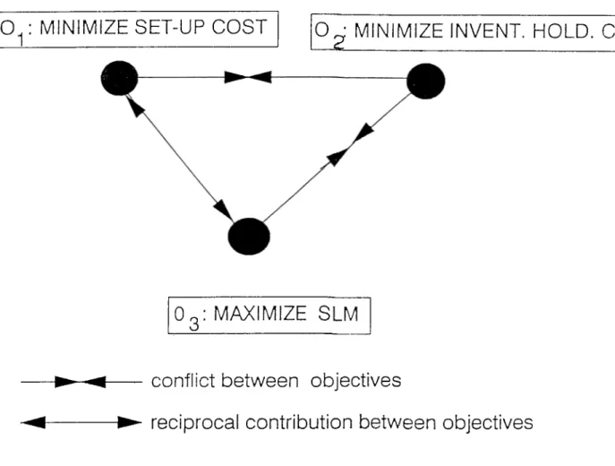
Using the above explanations, main objectives of a decision maker in PETKIM can be summarized as (figure 3.1):
• (9i: Minimize set-up cost per unit time
• O2: Minimize inventory holding cost per unit time
• O3: Maximize SLM
; MINIMIZE SET-UP COST
O · MINIMIZE INVENT. HOLD. C
O3: MAXIMIZE SLM
conflict between objectives
reciprocal contribution between objectives
Figure 3.1: Relations between the system of objectives under consideration
These measures can be defined as a function of the maximum inventory level and the reorder level which will be stated as the decision variables in the next chapter. The relations between these objectives are given in figure 3.1.
CHAPTER 3 PROBLEM UNDER CONSIDERATION 26
Total cost function is written as the sum of production and inventory hold ing cost. In order to keep up a certain service level, demand can be satisfied both by the production and by the inventory held. If more frequent start-ups and shut-downs are made by decreasing the production duration (lot size), then the total set-up cost is increased, but the inventory holding cost is decreased as the ’maximum (and hence the average) inventory level’ is decreased. .Similarly -at a predefined service level- decreasing the number of set-ups decreases the cost of production, but increases the cost of holding inventory as the average inventory level is increased this time. That means, 0 i and O2 are in con
flict meaning that the attem pt of achieving one of these objectives ‘adversely‘
affects the achievement of the other.
Obviously, one of the purposes of producing goods and holding in inventory is to satisfy the customer demand on time! Higher customer service level can be obtained by decreasing the number of stockouts in a planning horizon. Now let’s consider the ways of achieving this objective:
• One way of achieving less stockouts is to decrease the stockout pi'obabil-
ity in lead time by keeping a ’higher’ level of inventory against stockout
situations during the lead time. We know that this is achieved by increas ing the reorder level. This strategy increases the total cost as inventory holding costs are increased by keeping a higher level of safety stock. .A.s a result increasing the service level measure leads to an increase in the inventory holding cost. Thus O3 and O2 are in conflict. •
• Another way of decreasing the total number of stockouts is to decrease
the number of cycles in a planning horizon. We know that in every
cycle, stockouts may occur in lead times; thus decreasing the number of cycles will decrease the total number of stockouts in the planning horizon. Here we should note that, such a strategy will lead to long production durations and increased cycle times; which will decrease the total set-up cost in return. That means, increasing the service level measure leads to a decrease in the set-up cost. As a result, we should say that there is a reciprocal contribution between 0 \ and O3. i.e., the pursuit of 0 \
CHAPTER 3 PROBLEM UNDER CONSIDERATION 27
‘favorably‘ aiTects the achievement of O3 or vice versa. On the other hand, note that increasing the maximum inventory level again leads to increased inventory holding costs. Thus we show once more that O3 and
O2 are in conflict.
An important economic problem is caused by the fact that the total cost (as the sum of production cost and inventory holding cost) can not be mini mized while the customer satisfaction is maximized. These two objectives are again in conflict. More specifically, minimizing the total cost and maximizing the customer satisfaction can not be achieved at the same time. When the total cost is decreased (increased), then the customer satisfaction decreases (increases) too or vice versa. Hence a balance between these two objective variables should be established.
Briefly, main elements of our system of objectives that will be considered in throughout this thesis can be written of the form:
M in Total cost = Production cost T Inventory holding cost
M ax S L M = Percentage o f demand sa tisfie d per unit tim e
The above discussion briefly describes the problem of a plant manager (DM) in PETKIM. More specifically, as the set-up costs are too high in PETKIM, the plant managers avoid frequent shut-downs and start-ups so as to decrease production costs. However, long production duration causes increasing stock problems. Thus decreasing the total set-up costs in a planning period increases the inventory holding costs. However, the service level is rather high for the time being as any demand for an item can be immediately satisfied from the high level of inventory held.
Decision Variables:
W hat is needed in PETKIM is to make a trade-off between these objectives and develop an optimum control strategy that will minimize the sum of production cost and inventory holding cost while satisfying the customer demand. Thus
CHAPTER 3 PROBLEM UNDER CONSIDERATION 28
a mathematical model will be developed in which the decision variable(s) can be chosen among the state variables like:
1. Production Quantity
2. Production Duration
3. Cycle Time
4. Maximum Inventory Level
5. Reorder Level
6. Safety Stock Level, etc.
Depending on the properties of the inventory system and modelling tech nique, decision variable(s) can be any of the state variables defined above. Actually the production and inventory control mechanism is based on the de cisions about when to stop production and when to start again. In most of the inventory control models, the production duration is indirectly controlled by controlling the other state variables like the production quantity, maximum inventory level, reorder level etc. Actually, it may be easier for the decision maker to observe the incurring values of certain type of state variables. For instance in our problem, we suggest a production and inventory control model which works on the maximum inventory level and the reorder level. Production is stopped when the inventory level reaches a maximum level and it is started again when it drops to reorder level.
Note that if the decision variable is the production duration, all other state variables will stand for the consequence variables; that means the production quantity, cycle time, maximum inventory level etc. will take values as a func tion of the production duration. Similarly, depending on the mathematical relations between these state variables, safety stock comes out to be a conse quence variable which is evaluated according to the value of the reorder level.
For the PETKIM production and inventory system, we take the maximum inventory level and the reorder level as the decision variables, instead of any
CHAPTER 3 PROBLEM UNDER CONSIDERATION 29
other state variables. This enables us to establish a robust production and inventory control model where the losses incurred by parameter estimation errors are very low. The details of this analysis is given in the next chapters.
C hapter 4
M O D EL C O N S T R U C T IO N
In this section we deal with sizing and timing decisions for production lots and more precisely with mathematical models which offer an optimum production plan, nainely a lot sizing strategy.
Our mam model is a ’’bi-objective decision making’ model. The first objec tive is to minimize the sum of production and inventory holding costs whereas the second objective is to maximize the customer sati.sfaction using a service level measure. In this approach, total cost can be expressed as a function of two decision variables: maximum inventory level (7) and the reorder level (g)
Total Cost = TC{ I , g )
For any inventory control plan, it is possible to find a value measure for the
ratio of demand satisfied per unit time. In other words, SLM is again a function
of maximum inventory level and the reorder level.
Service Level M easure = SLA4{I, g)
Then the main elements of our system of objectives comes out to be two dif ferent functions of the same decision variables / and g.
Depending on the values of the decision variables, a production and inven tory control model is defined. This main model is somewhat similar to an (S,s)
CHAPTER 4. MODEL CONSTRUCTION 31
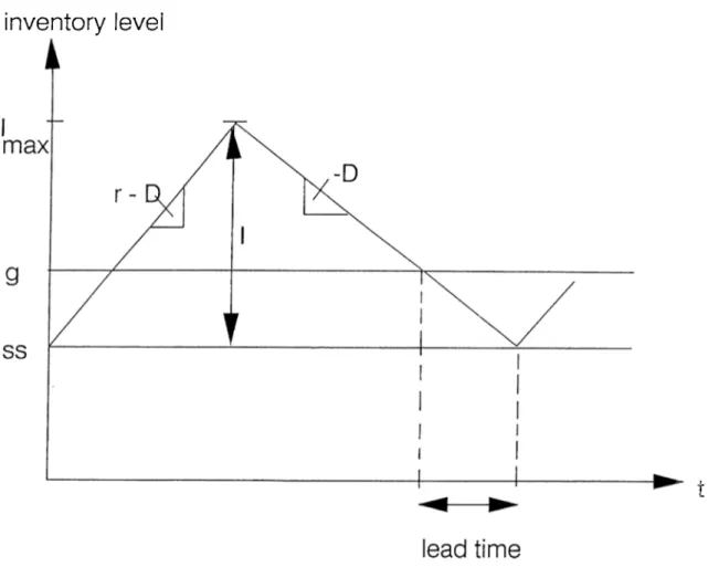
inventory control policy model, which operates on the inventory position. A re generative process -as in the case of (S,s) systems- exists in the so-called ’main model’, which operates in the following way: An order to start producing an item is given when the inventory level drops to a ’reorder’ level, g (figure 4.1 ). Production starts after a lead time and the difference between production and demand is added to the inventory. Production continues until the inventory level reaches a ’maximum’ level {—I + ss), then it is stopped until the inventory level drops to the reorder level {g) and a new cycle begins and so on.
inventory level
Figure 4.1: Change in the inventory level when the S P I L model is applied.
In this proposed model, the inventory control mechanism is based on two decision variables: the m ax im u m in v e n to ry level and the re o rd e r level.