THE HAZARDOUS WASTE LOCATION-ROUTING PROBLEM
A THESIS
SUBMITTED TO THE DEPARTMENT OF INDUSTRIAL ENGINEERING
AND THE INSTITUTE OF ENGINEERING AND SCIENCES OF BILKENT UNIVERSITY
IN PARTIAL FULFILLMENT OF THE REQUIREMENTS FOR THE DEGREE OF
MASTER OF SCIENCE
by Sibel Alumur December 2003
Asst. Prof. Bahar Y. Kara (Principal Advisor)
I certify that I have read this thesis and that in my opinion it is fully adequate, in scope and in quality, as a thesis for the degree of Master of Science.
Assoc. Prof. Osman Oğuz
I certify that I have read this thesis and that in my opinion it is fully adequate, in scope and in quality, as a thesis for the degree of Master of Science.
Asst. Prof. Oya Ekin Karaşan
Approved for the Institute of Engineering and Sciences:
Prof. Mehmet Baray
iii
ABSTRACT
THE HAZARDOUS WASTE LOCATION-ROUTING PROBLEM Sibel Alumur
M.S. in Industrial Engineering Supervisor: Assist. Prof. Bahar Y. Kara
December 2003
As a result of high industrialization and technology hazardous waste management problem has now become an unavoidable problem of the world. Hazardous waste management involves collection, transportation, treatment and disposal of hazardous wastes. In this thesis, the existing models in the literature are analyzed in terms of applicability. A new multiobjective location-routing model is proposed by combining the applicable aspects from different models. Our model also includes the constraints that reflect certain requirements that have been observed in the literature but could not been incorporated into the models correctly together with the additional constraints that we propose. The aim of the model is to decide on the following questions: where to open treatment centers with which technologies, where to open disposal centers, how to route different types of hazardous wastes to which of the compatible treatment technologies, and how to route waste residues to disposal centers. The model has two objectives of minimizing total cost and minimizing transportation risk. A large scale implementation of the model in the Central Anatolian Region of Turkey is presented.
Keywords: Hazardous waste, Facility Location, Routing, Multiobjective Model.
TEHLİKELİ ATIKLAR İÇİN YER SEÇİMİ VE ROTALAMA PROBLEMİ Sibel Alumur
Endüstri Mühendisliği Yüksek Lisans Tez Yöneticisi: Assist. Prof. Bahar Y. Kara
Aralık 2003
Tehlikeli atıkların kontrolü hızlı gelişen teknoloji ve endüstri sonrasında dünyada kaçınılamayacak bir problem haline gelmiştir. Tehlikeli atıkların kontrolü, tehlikeli atıkların toplanması, taşınması, arıtılması ve bertarafını içermektedir. Bu çalışmada litetatürdeki matematiksel modeller uygulanabilirlik yönünden incelenmiştir. Literatürdeki uygulanabilir kısıtlar da göz önüne alınarak yeni bir çok amaçlı matematiksel model sunulmuştur. Sunulan bu model, bizim önerdiğimiz yeni kısıtlarla literatürde önerilen ama matematiksel modellere yansıtılamayan ksıtları da içermektedir. Model şu sorulara cevap aramaktadır: arıtma tesisleri hangi teknolojilerle nereye açılmalı, bertaraf tesisleri nereye açılmalı, farklı cinsteki tehlikeli atıklar uyumlu arıtma teknolojilerine nasıl rotalanmalı ve kalan atıklar bertaraf tesislerine nasıl rotalanmalı. Modelin biri maliyetin enküçüklenmesi, diğeri riskin enküçüklenmesi olmak üzere iki tane amacı vardır. Modelin Türkiye’nin İç Anadolu Bölgesi’nde büyük ölçekli bir uygulaması sunulmuştur.
Anahtar Kelimeler: Tehlikeli atık, Yer Seçimi, Rotalama, Çok Amaçlı Matematiksel Model
v
I would like to express my sincere gratitude to Asst. Prof. Bahar Yetiş Kara for all the encouragement and trust during my graduate study and for her unique guidance. I feel lucky to have worked with a supervisor like her.
I am indebted to members of my dissertation committee: Assoc. Prof. Osman Oğuz, Asst. Prof. Oya Ekin Karaşan for showing keen interest in the subject matter and accepting to read and review this thesis. Their remarks and recommendations have been very helpful.
I am mostly indebted to my family. I was first to earn an M.S. degree in my whole family after my dearest father Demir Alumur. I am also grateful to my mother Nural Alumur and brother Volkan Alumur for their support. I would like to thank Talha Akçaboy for his friendship, morale support and endless love.
Finally, I would like to express my gratitude to my whole friends. Life and the graduate study would not have been bearable without them. I would first like to thank Evren Emek with whom I started the graduate study and shared every memory. I am also thankful to Ayışığı Sevdik, Ayça Yetere, Pınar Tan, and Ahmet Tuzcu, all the members of the room 327 and all my other friends who have always been there for me.
vii CONTENTS
1 INTRODUCTION...1
2 LITERATURE REVIEW ...6
3 MODEL DEVELOPMENT...16
3.1 Combinatorial Formulation and Complexity ...20
3.2 The mixed-integer programming model...22
4 APPLICATION IN TURKEY ...29
5 CONCLUSIONS AND FUTURE RESEARCH DIRECTIONS ...42
BIBLIOGRAPHY ...45
APPENDIX ...50
A LOCATIONS OF ADMINISTRATIVE DISTRICTS...51
1.1 Hazardous waste management problem ... 4
3.1 Decision variables of the mathematical model... 23
4.1 Administrative districts and highway network in the region ... 29
4.2 Selected 112 districts of the Central Anatolian Region ... 31
4.3 Trade-off curve... 41
A.1 Selected administrative districts, their node numbers and the corresponding locations... 51
ix LIST OF TABLES
2.1 Summary of the hazardous waste location-routing literature ... 14
4.1 Parameters of the three cases in the application... 34
4.2 Minimum cost and minimum risk solutions for 15 candidates... 35
4.3 Treatment and disposal centers' locations with 15 candidate sites ... 36
4.4 Cost and risk values for given linear combinations and deviations from the minimum for 15 candidates... 38
4.5 Average, maximum and minimum CPU times in hours for 15 candidate solutions... 39
4.6 CPU times in hours, number of iterations and number of nodes of 15 candidate solutions ... 39
4.7 Average, maximum and minimum CPU times in hours for 20 candidate solutions ... 40
A.1 Selected 112 administrative districts and their corresponding node numbers, populations and provinces that they belong to ... 52
C h a p t e r 1
INTRODUCTION
A waste can be characterized as hazardous if it possesses any one of the following four characteristics: ignitability, corrosivity, reactivity or toxicity. The vulnerability of and the avoidance from the hazardous wastes comes from the word ‘hazardous’ meaning that those kinds of wastes may cause threat to human health, welfare or environment. The hazardous wastes, which are usually the waste by-products of our industrial processes, present immediate or long-term risks to humans, animals, plants, or the environment which must be avoided. Many types of businesses generate hazardous wastes. Some are small companies that are located in community such as dry cleaners, auto repair shops, hospitals, exterminators, and photo processing centers; where some hazardous waste generators are relatively larger companies like chemical manufacturers, electroplating companies, and petroleum refineries. In addition to industries, there are hazardous household wastes as well such as batteries, gasoline, antifreeze, oil-based paints and thinners, household cleaning products and pesticides.
The hazardous waste management problem has now become an unavoidable problem of the world mainly as a result of high industrial and technological developments. Even though the new trend in the world is not to produce any hazardous wastes, by waste minimization, or by using replaceable materials, still huge amounts of hazardous wastes which have to be managed somehow
CHAPTER 1 INTRODUCTION
2 are being produced each day. Unfortunately, much of the produced hazardous wastes are disposed of in a manner that does not meet basic standards of environmental safety in the world. The objective of the hazardous waste management problem stated by Nema and Gupta [29] is “to ensure safe, efficient and cost effective collection, transportation, treatment and disposal of wastes”. But the main question still remains valid: How are we going to manage the hazardous wastes?
The solution to the hazardous waste management problem may differ when we look from different perspectives as usually multiple stakeholders are involved, such as government and private companies. Thus, there are various objectives while managing the problem in a safe and cost effective manner. For example for a carrier firm the best solution of the hazardous waste management problem would be the one with the least cost, while for the government the best solution would be the one with least risk. The decision maker should select the best compromising solution among these different objectives.
The hazardous waste treatment facilities (such as incinerators) and disposal facilities (such as landfills) are usually considered as undesirable facilities in the literature. This is because; nobody wants to have an incinerator or a landfill at their backyard, the syndrome known as NIMBY (Not in my backyard). Unfortunately, it is not possible to satisfy everyone because as we move the problem away from one population we move it closer to another one. This makes the problem harder as there will always be some kind of public opposition to the solution.
Another aspect of the hazardous waste management problem is that various kinds of hazardous wastes are generated every day, which may or may not be managed together. Again there are various treatment technologies which may
be specific to the kind of the hazardous waste to be treated such as chemical treatment technologies, or may service more than one type of hazardous wastes such as incinerators. The compatibility issues are also important. There are wastes which are not compatible with certain kinds of treatment technologies. For example, a highly reactive chemical waste can not be incinerated. Any proposed solution should also include these real life aspects of the hazardous waste management problem.
The hazardous waste treatment facilities are usually not the ultimate disposal centers. After the treatment process the produced waste residues, which are no longer hazardous, should be disposed off. The amount of produced waste residue is almost always dependent on the employed treatment technology. For example, the volume or mass reduction after incineration is significantly higher than the volume or mass reduction after chemical disinfection. As the transportation cost of these waste residues is another issue, location of the disposal facilities, and the routes of the waste residues should also be determined while locating the treatment facilities.
Another important issue is recycling. Recycling should be encouraged for both the produced hazardous wastes and the waste residues, if possible, which is usually dependent on the hazardous waste type and the employed treatment technology.
As a summary, a solution to the hazardous waste management problem should decide on the following questions: Where to open treatment centers with which technologies, where to open disposal centers, how to route different types of hazardous wastes to which of the compatible treatment technologies, and how to route waste residues to disposal centers.
CHAPTER 1 INTRODUCTION
4 So the overall picture (Figure 1.1) of the hazardous waste management problem starts from the generation of hazardous wastes, then the non-recycled amount of hazardous wastes are to be routed to the compatible treatment technology in the treatment facility which is to be located. After the treatment process, the non-recycled amount of waste residues are to be routed to the ultimate disposal facility which is again to be located.
Figure 1.1 Hazardous waste management problem
In this study, our aim is to find a good solution to the hazardous waste management problem. For this, firstly, the existing models in the literature are analyzed in terms of applicability. Secondly, a new multiobjective location-routing model is developed by combining the applicable aspects from different models in the literature. The model also includes the constraints that reflect certain requirements that have been observed in the literature but could not have been incorporated into the models correctly, together with the additional constraints that we propose. Lastly, the performance of the model is experimented in the Central Anatolian Region of Turkey.
Recycle
Generation Node
Recycle
Treatment
Center Disposal Center
Hazardous Waste
The remainder of this thesis is outlined as follows: In the next chapter, the existing literature on the hazardous waste location-routing problem is reviewed with emphasis on similarities, differences and deficiencies. The third chapter is devoted to the mathematical model that we propose. The forth chapter presents a large-scale implementation of the model in Turkey. Lastly, in chapter five some concluding results and suggestions for future research are provided.
6
C h a p t e r 2
LITERATURE REVIEW
As stated earlier, the hazardous waste management problem has recently become significantly important mainly after the rapid technological and industrial developments. With increasing technology and industry the problem of managing hazardous wastes comes as a by-product. Thus the papers related to hazardous waste management increases mainly after the year 1990.
The earliest effort to manage the hazardous waste problem is by Peirce and Davidson [30]. They aimed to identify the cost effective configuration of transportation routes, transfer stations, processing facilities and secure long-term storage impoundments. However, they only considered the allocation aspect of the problem in which they decided on the optimal routing strategy. They applied Environmental Protection Agency’s (EPA) Waste Resource Allocation Program (WRAP) to a selected region. Another paper dealing with the allocation aspect of the hazardous waste management problem is by Jennings and Scholar [21]. They have considered many real life aspects of the problem, such as compatibility of hazardous wastes with technology, establishment of different technologies at different sites, risk assessment for each type of hazardous waste, and the ultimate disposal problem in addition to the treatment problem. Although this paper did not include the location aspect of the hazardous waste management problem, the proposed ideas are present
in most of the recent papers dealing with the hazardous waste location-routing problem.
Some studies in the literature are only concerned with the routing aspect of the hazardous waste management problem. These studies try to find the optimal routes of hazardous materials (hazmat) which minimize risk between the given origin-destination pairs. Various attitudes and risk measures are used in hazmat papers. Two of the risk measures that are commonly used are the societal risk and the population exposure. Societal risk is the product of probability of a hazardous waste accident occurrence times the consequences of that accident and the population exposure is the number of people exposed to hazardous wastes. [17]
The hazardous waste management problem is also handled in location literature in locating treatment, or disposal facilities. The treatment facilities, such as incinerators, and the disposal facilities, such as landfills, are usually considered as undesirable facilities in the location literature. There is quite a literature on undesirable facility location [15]. In the location of undesirable facilities the aim is to minimize the nuisance and the adverse effects on the existing facilities or population centers. Although, the service cost of the undesirable facility to be located increases when the facility is located far from the population centers, the undesirability of the facility usually seemed to be more important.
The first study in the undesirable facility location literature is by Church and Garfinkel [6] in 1978, in which they tried to locate a single undesirable facility on a network by maximizing the sum of distances between the population centers and the facility to be located. This model is later named as the ‘maxisum’ model in the literature. After, Church and Garfinkel [6] many
CHAPTER 2 LITERATURE REVIEW
8 authors address the maxisum problem in following years. (Hansen, Peeters and Thisse [19], Melachrinoudis and Cullinane [28], Karkazis [22], Karkazis and Papadimitriou [23]) However, a disadvantage of the maxisum model is that it may result in a solution where the optimum location is in the immediate neighborhood of a population center. Thus, there is a more preferred model in the literature which is called the ‘maximin’ model. The aim of the maximin model is to locate a facility in a given region so that the minimum distance between this facility and the population centers is to be maximized. There are over 35 papers dealing with the ‘maximin’ model and its variations in the undesirable facility location literature. Some examples are: Dasarathy and White [9], Drezner and Wesolowsky [10, 11, 12], Melachrinoudis and Cullinane [26, 27, 28], Erkut and Öncü [16], Rangan and Govindan [32], Mehrez, Sinuany-Stern and Stulman [25], Appa and Giannikos [1].
Apart from the ‘maxisum’ and ‘maximin’ models there is another model which is relatively new and less preferred. This new model is called the ‘minimum covering’ model and its aim is to find a location for a new facility such that the total number of population centers within a specified distance is minimized. (Sung and Joo [35], Drezner and Wesolowsky [13], Berman, Drezner and Wesolowsky [4], Plastria and Carrizosa [31])
Erkut and Neuman [15] stated in their survey on undesirable facility location that “the location of an undesirable facility is almost always connected with an establishment of an undesirable network.” This is also the case for hazardous waste treatment facilities as it is connected with an undesirable hazardous waste transportation network. Thus, if one wants to minimize the risk or nuisance due to the location of the facility one should also include the nuisance or risk due to transportation and model the location-routing problem simultaneously.
The main focus in this literature section will be on the combined location-routing models on hazardous wastes, as our study also tends to model the location-routing problem simultaneously.
The location-routing term is a synonym for the integration of facility location and vehicle routing problems. Here we find it useful to state the difference between the well known location-routing problem and the hazardous waste location-routing problem. The aim of the standard location-routing problem is to find the optimal allocation and routing strategy. In this location-routing problems, the customers are going to be served from the facilities which are going to be located and the routes that the vehicle would follow from the facility to the customers are going to be determined. In this problem the vehicle is allowed to visit more than one customer at a time. One may refer to a recent review on location-routing problems by Erdoğan, Erdoğan and Tansel [14] for detailed explanation on the standard location-routing problems. In the hazardous waste location-routing problem the generated hazardous wastes are allocated to treatment facilities which are to be located and each generation center has its own optimal path to the treatment facility. The models in the hazardous waste location-routing literature are not concerned with the route of the vehicles that transport these wastes to the assigned treatment facilities. In a way, hazardous waste location-routing literature deals only with the location of treatment facilities and allocation of generation centers to these treatment facilities. It is trivial that after locating the treatment facilities, the hazardous waste generation centers would transport their wastes on their shortest (minimum cost) path. However, the hazardous waste location-routing models are usually multiobjective programming models, there is a risk objective in addition to the cost objective and it is the risk objective that may change the path that is to be selected. As a result, the aim of the hazardous waste location-routing problem is not to solve the vehicle routing problem, but
CHAPTER 2 LITERATURE REVIEW
10 to find the optimal paths in allocating the generation centers to treatment facilities. It may be more reasonable to call our problem as the hazardous waste allocation problem instead of calling hazardous waste location-routing problem. However, we prefer to use the terminology that has appeared in the literature.
The hazardous waste location-routing models in the literature are usually multiobjective mixed integer programming models which can be solved by numerous software by employing the common simple multiobjective techniques. In these hazardous waste location-routing models the aim is to model the problem effectively. Thus, the studies in this area vary mainly due to the presented models instead of the solution procedures.
The fist effort in modeling the location-routing problem simultaneously is by Zografos and Samara [37]. They proposed a multiobjective model for only one type of hazardous waste which minimizes travel time, transportation risk and disposal risk in which they used the goal programming technique. The disadvantages of their model are that each population center is affected only from its nearest opened treatment facility, and every source node can send its generated hazardous waste to only one treatment facility. Later, List and Mirchandani [24] also developed a multiobjective model for again a single type of hazardous waste with three objectives of minimizing risk, minimizing cost and maximizing equity in which the aim is to find the Pareto optimal solutions. They located storage and disposal facilities in addition to treatment facilities. They proposed a new risk impact function which is inversely proportional to the square of the distance; however they could not use this new complex risk function while applying the model to the capital district of Albany, NY.
Revelle, Cohon and Shobrys [33] minimized a convex combination of cost and risk, where cost measure is taken as the distance traveled and risk measure is taken as the population exposure, to model the location-routing problem for a single type of hazardous waste. Their simple and easily applicable model aims to find the location of disposal sites, which sources are assigned to a particular disposal site, and which routes the waste follow from each source to its assigned destination.
Alidi [2] presented an integer goal programming model for different types of generated hazardous wastes, and for different time periods. They considered recycling from treatment centers where the recyclable materials can be recovered and sold to markets. Their location-routing model locates incinerators for treatment, landfills for disposal and markets for recycling, and decides on the routes that the hazardous wastes follow to these facilities. Stowers and Palekar [34] only considered risk in their location-routing model for a single type of hazardous waste. They used population exposure as a surrogate for risk in minimizing the risk both due to location and transportation. The location of the treatment facility is not restricted to some known set of potential sites in their model. This may be unrealistic as most of the locations may not be suitable from an environmental perspective. For example, for the location of landfills, the site should be far away both from the rivers, lakes and also from the groundwater supplies to prevent the probable contamination that may be caused by leakages.
Jacobs and Warmerdam [20] presented a location-routing model for one type of hazardous waste. They modeled the problem as a continuous network flow problem, and locate the storage and disposal sites while minimizing the linear
CHAPTER 2 LITERATURE REVIEW
12 combination of cost and risk in time. They defined risk as the total probability of release causing accident during transportation, storage or disposal.
Current and Ratick [8] presented a mixed-integer programming location-routing model for a single type of hazardous waste which minimizes cost, risk and maximizes equity. They analyzed the transportation and facility location components of risk and equity separately. However, their formulation assumes that wastes cannot be transported through a generation node or a facility node. Wyman and Kuby [36] also presented a multiobjective mixed-integer programming location-routing model for a single type of hazardous waste with the same objectives where technology choice for treatment facilities is also considered.
Alidi [3] presented another paper which focuses only on the wastes of petrochemical industry. He stated that there are different stake-holders with different goals, thus he used the Analytical Hierarchy Process (AHP). The presented model is only an allocation model, but it may be valuable as different aspects of the hazardous waste management is considered such as recycling, waste minimization, and energy production as a result of incineration.
Giannikos [18] considered four objectives in his multiobjective location-routing model in which he used the goal programming technique. These objectives are minimization of cost, minimization of total perceived risk, equitable distribution of risk among population centers and the equitable distribution of disutility caused by the operation of the treatment facilities. Nema and Gupta [29] proposed another model for the hazardous waste location-routing problem. They used a composite objective function consisting of total cost and total risk, where total cost and risk includes treatment,
disposal and transportation costs and risks. They proposed two new constraints which are waste-waste, and waste-technology compatibility constraints. Waste-waste compatibility constraint ensures that a waste is transported or treated only with a compatible waste, and waste-technology compatibility constraint ensures that a waste is treated only with a compatible technology. However, they could not implement these constraints into the proposed mathematical model.
The hazardous waste location-routing literature is summarized in Table 2.1. This table only summarizes the objectives of the presented models in the literature and specifies if the presented models are suitable for a single hazardous waste type or for multiple hazardous waste types. As it is stated before, the aim of the papers in the hazardous waste location-routing literature is to present a realistic, and applicable mathematical model. Thus all of the papers in this area suggested using an optimization software, employing the common and simple multiobjective solution techniques. None of the papers in the literature proposed a heuristic for the hazardous waste location-routing problem.
As a synthesis of the existing literature we may say that minimization of cost and minimization of risk are the most commonly employed objectives. Some authors also used equity as an objective, which may result in locating more treatment or disposal facilities so that the population is equally exposed to risk. Most of the papers only considered one type of hazardous waste, which is a significant simplification as the hazardous waste management is concerned with various types of hazardous wastes. Different risk measures are used in the papers, where the most popular ones are the population exposure and societal risk.
CHAPTER 2 LITERATURE REVIEW
14
Year Authors Objectives Hazardous
waste type 1990 Zografos and
Samara [37]
Minimization of transportation risk, disposal risk and travel time
single
1991 List and
Mirchandani [24]
Minimization of risk, cost and maximization of equity
single
1991 ReVelle, Cohon and Shobrys [33]
Minimization of convex combination of cost and risk
single
1992 Alidi[2] Various goals, used goal programming technique
multiple
1993 Stowers and Palekar [34]
Minimization of total exposure of transportation and total exposure of long term storage
single
1994 Jacobs and Warmerdam [20]
Minimization of linear combination of total cost and total risk
single
1995 Current and Ratick [8]
Minimization of risk, cost and maximization of equity
single
1996 Alidi[3] Various goals, used Analytical Hierarchy Process
multiple
1998 Giannikos [18] Min. of total operating cost, total perceived risk, equitable
distribution of risk and disutility
single
1999 Nema and Gupta [29]
Minimization of total cost and total risk of transportation, treatment and disposal operations
multiple
Table 2.1 Summary of the hazardous waste location–routing literature A deficiency of the hazardous waste location routing literature is that the models usually do not reflect the real life situation. The single waste type assumption presented in most of the papers is such an example. Apart from the single waste type assumption; all the models except one do not consider
different treatment technologies, and the waste types that are compatible with those different technologies. Also recycling issues did not appear in most of the hazardous waste location-routing papers, which is again an important deficiency of the presented models in the literature. Another deficiency of the literature is that it lacks large scale applications. Most of the papers present applications with small instances, such as with 10 or 15 node networks and with 2 or 3 candidate sites.
Another common trend in the literature is to ignore the waste residue problem, which includes the routing of waste residues and location of disposal centers, as waste residues are no longer hazardous. However, the transportation costs of waste residues should be included while calculating hazardous waste management costs and thus if cost is to be minimized one should also include the costs related to waste residue management.
As a result, the hazardous waste location-routing literature lacks a mathematical model which includes all the stated real life aspects of the hazardous waste management problem.
16
C h a p t e r 3
MODEL DEVELOPMENT
In this section, we propose a mathematical model whose aim is to treat all the generated hazardous wastes and dispose all the generated waste residues in a safe and cost effective manner.
The treatment of generated hazardous wastes and the disposal of waste residues at certain sites require a transportation network, on which the hazardous wastes and waste residues are routed. The nodes of this transportation network may be a generation node, a transshipment node (a node junction), a potential treatment facility, a potential disposal facility or any combination of these stated nodes. It is assumed that the potential sites for treatment and disposal facilities have already been identified on this transportation network.
There is cost in transportation, treatment and disposal operations and there is risk posed to the environment in transporting hazardous wastes. Then, the aim is to treat and dispose the generated hazardous wastes with minimum cost and minimum risk to the environment.
For each link of the transportation network the cost of transporting one unit of hazardous waste or one unit of waste residue are known, which are assumed to be directly proportional to the network distance used. The transportation cost of hazardous wastes and waste residues may be different as special trucks or
containers may be needed in transporting hazardous wastes, while the waste residues can be transported casually as domestic waste as they are no longer hazardous.
There is fixed cost of locating treatment and disposal facilities. This cost, which is usually dependent on the employed treatment technology or size of the facility to be located or any various factors, is again assumed to be known. The transportation of hazardous wastes poses some risk to the environment. Different measures of risk can be used to estimate this transportation risk. For example, one may use societal risk (the product of the probability of a hazardous waste accident occurrence times the consequences of that accident) or population exposure (the number of people exposed to hazardous wastes) as a risk measure. For our proposed model the only assumption about the risk measure is its linearity. The presented model uses population exposure as a surrogate for risk measure for ease of application and data availability.
The proposed model can manage different types of hazardous wastes and different treatment technologies. The important parameter in managing different types of hazardous wastes with different treatment technologies is the compatibility parameter. There are various treatment technologies which may be specific to the kind of the hazardous waste to be treated such as chemical treatment technologies, or may service more than one type of hazardous waste such as incinerators. As it is mentioned in Chapter 2, even though the necessity of the compatibility parameter is observed in the literature [29], it could not have been incorporated into the suggested mathematical models. It is assumed that the hazardous waste types that are compatible with which of the given treatment technologies are known.
CHAPTER 3 MODEL DEVELOPMENT
18 Our model also allows recycling which can either be adopted at a generation node, or at a treatment center. The recycling percent of a hazardous waste type from a generation node is assumed to be known for each type of hazardous waste at each generation node. The recycling percent of the waste residues from the treatment centers are also assumed to be known.
The proposed mathematical model for hazardous waste location-routing problem can be stated as follows: Given a transportation network and the set of potential nodes for treatment and disposal facilities, find the location of treatment and disposal centers and the amount of shipped hazardous wastes and waste residues in the given transportation network so as to minimize the total cost and the transportation risk.
The proposed model is formulated as a multiobjective mixed integer programming model with two objectives of (1) minimizing total cost, and (2) minimizing transportation risk. The model is subjected to the conservation of flow constraints for both hazardous wastes and waste residues. Conservation of flow constraint for a given node ensures that the amount of hazardous wastes (or waste residues) coming to that node is equal to the amount leaving that node. Another important constraint is the mass balance constraint which is usually not present in the other transportation problems. During mass balance the treated and non-recycled hazardous wastes are transformed into waste residues. Mass balance constraint ensures that all the waste residues generated after the treatment process are to be disposed off. There is a minimum amount requirement constraint which ensures that a treatment technology is opened only if the minimum amount required for that technology is available. The minimum amount requirement constraint is necessary in real life, as some technologies need at least a specified amount of hazardous waste to operate. The compatibility constraint, the necessity of which is explained before, is also
incorporated into the model. Apart from the above constraints there are also the capacity constraints.
The following indices and parameters are used in the mathematical model: Given;
N = (V, A) Transportation network G = {1,…,g} Generation nodes
T = {1,…,t} Potential treatment nodes D = {1,…,d} Potential disposal nodes Tr = {1,…,tr} Transshipment nodes W = {1,…,w} Hazardous waste types Q = {1,…,q} Treatment technologies Parameters:
ci,j cost of transporting one unit of hazardous waste on link (i,j) Є A
czi,j cost of transporting one unit of waste residue on link (i,j) Є A
fcq,i fixed annual cost of opening a treatment technology q Є Q at treatment
node i Є T
POPwij number of people in a given radius for hazardous waste type w Є W
CHAPTER 3 MODEL DEVELOPMENT
20 gw,i amount of hazardous waste type w Є W generated at generation node i
Є G
αw,i recycle percent of hazardous waste type w Є W generated at
generation node i Є G
βw,i recycle percent of hazardous waste type w Є W treated at treatment
node i Є T
rw,q percent mass reduction of hazardous waste type w Є W treated with
technology q Є Q
tq,i capacity of treatment technology q Є Q at treatment node i Є T
tq,im minimum amount of hazardous waste required for treatment
technology q Є Q at treatment center i Є T dci disposal capacity of disposal site i Є D
p number of disposal sites to be opened
comw,q 1 if waste type w Є W is compatible with technology q Є Q;
0 otherwise
3.1 Combinatorial Formulation and Complexity
The hazardous waste location-routing problem is to open a subset of treatment and disposal facilities in order to minimize the total cost and risk, given that all the hazardous wastes that are generated has to be treated and all the generated waste residues has to be disposed off. The generated and non-recycled amount of hazardous wastes are transported to the compatible treatment facilities
which are to be located. Then the non-recycled amount of waste residues that are generated in the treatment centers are to be disposed of in the disposal facilities which are again to be located. An instance of the hazardous waste location-routing problem is specified by integers m, n, k, w, q and p, two m × n cost matrices C = {ci,j} and CZ = {czi,j}, a q × m fixed cost matrix FC =
{fcq,i}, w amount of m × n population matrices POP = {popi,j}, a w × n matrix
of amount of generated hazardous wastes G = {gw,i}, a w × n matrix of recycle
percentages of hazardous wastes αw,i, a w × m matrix of recycle percentages of
waste residues βw,i, a w × q matrix of percent mass reductions rw,q, a q × m
matrix of capacities of treatment centers tq,i, a q × m matrix of minimum
amount requirement for technologies tq,im, a 1 × k matrix of disposal center
capacities dci, a w × q matrix of compatibility comw,q and p which is the
number of disposal centers to be opened.
Theorem 3.1 The hazardous waste location-routing problem is NP-hard.
Proof: First we need to introduce the uncapacitated facility location (UFL) problem. The UFL problem is to open a subset of facilities in order to
maximize total profit (or minimize cost), given that all demand has to be satisfied. An instance of the UFL problem is specified by integers m and n, an n × m cost matrix Cost = {costi,j} and a 1 × m fixed cost matrix Fixed =
{fixedj}. The UFL problem is NP-hard. [7]
We now reduce the hazardous waste location-routing problem to the UFL problem. Construct an instance of the hazardous waste location-routing problem with the following parameters. Let | W| = 1 (one waste type), | Q| = 1
(one treatment technology), | T| = m (m candidate sites for treatment facilities),
| D| = m (m candidate sites for disposal facilities) and p = 0 (no disposal facility is to be located). Also let czi,j = 0 for all i and j (no cost in transporting waste
CHAPTER 3 MODEL DEVELOPMENT
22 residues), gw,i = 1 for all w and i (all nodes generate 1 unit of hazardous
waste), αw,i = 0 and βw,i = 0 for all w and i (no recycling in both generation
nodes and treatment centers), rw,q = 1 for all w and q (no waste residues are
produced), tq,im = 0 for all q and i (no minimum capacity requirement for
treatment technologies), and let tq,i and dci be infinity (no capacity restriction
for treatment technologies and disposal centers) and comw,q = 1 for all w and q
(no compatibility restriction). Then, this instance of the hazardous waste location-routing problem is to open a subset of facilities in order to minimize a ‘cost’ given that all hazardous wastes that are generated have to be treated, and it is specified by integers m and n, an m × n cost matrix Cost = {costi,j = λ × ci,j
+ (1-λ) × popi,j}, and a 1 × m fixed cost matrix Fixed = {fci}. The
combinatorial formulation of this instance of the hazardous waste location-routing problem is equivalent to the combinatorial formulation of the UFL problem. This proves that the hazardous waste location-routing problem is NP-hard. ٱ
3.2 The Mixed-Integer-Programming Model
We now propose a new mixed-integer-programming mathematical model for the hazardous waste location-routing problem. The following decision variables are used in the mathematical model:
Decision Variables:
xw,i,j amount of hazardous waste type w transported through link (i,j)
zi,j amount of waste residue transported through link (i,j)
yw,q,i amount of hazardous waste type w to be treated at treatment
di amount of waste residue to be disposed off at disposal node i
fq,i 1 if treatment technology q is established at treatment node i;
0 otherwise
dzi 1 if disposal site is established at disposal node i;
0 otherwise
The decision variables and some parameters of the proposed model are schematically shown in Figure 3.1. In the model, the non-recycled amount of generated hazardous wastes ((1-αw,i)gw,i) are to be routed (xw,i,j) to the
compatible treatment technology in the treatment facility (yw,q,i) which is to be
located (fq,i). After the treatment process, the non-recycled amount of waste
residues are to be routed (zi,j) to the ultimate disposal facility which is again to
be located (di).
Figure 3.1 Decision variables of the mathematical model
α
w,ig
w,iGeneration Node
β
w,qy
w,q,iTreatment
Center Disposal Center
x
w,i,jz
i,jg
w,iy
w,q,id
iCHAPTER 3 MODEL DEVELOPMENT 24 (9) D) (V i 0 (8) T) (V i 0 (7) p (6) T i Q, q W, w com t (5) T i Q, q t (4) D i dc (3) T i Q, q t (2) V i ) -)(1 r -(1 (1) V i W, w )g -(1 subject to POP Minimize OR fc cz c Minimize q w i q w, i q, w m i q, i w q,i A i) (j, :j q w :j(i,j)A q w, q w, A j) (i, : j j :(j,i)A q i w, i w, A j) (i, w j i, w, i q q,i A j) (i, i,j A j) (i, w i,j − ∈ = − ∈ = = ∈ ∈ ∈ ≤ ∈ ∈ ≥ ∈ ≤ ∈ ∈ ≤ ∈ − = − ∈ ∈ + − = + +
∑∑
∑
∑
∑
∑
∑∑
∑
∑
∑
∑
∑ ∑
∑∑
∑
∑ ∑
∈ ∈ ∈ ∈ ∈ ∈ ∈ i i q, w, i i q, w, i q, i q, w, i i i q, i q, w, i j, j i, i i q, w, i q, w, i j, w, j i, w, j i, w, i q, j i, j i, w, d y dz y f y dz d f y z z d y y x x x f z x β αFirst objective is the cost objective minimizing the total cost of transporting hazardous wastes and waste residues, and fixed annual cost of opening a treatment technology. The fixed cost of opening a disposal facility is not present in the objective function as no matter what the fixed cost is the model is going to locate exactly p disposal facilities.
The second objective is the risk objective minimizing the transportation risk which is measured with the population exposure. The amount of shipped hazardous wastes on a given link times the amount of people living along a given bandwidth on that link is to be minimized. As the given bandwidth may differ for different hazardous waste types the equation is summed for all hazardous waste types.
First constraint is the flow balance constraint for hazardous wastes. This constraint ensures that all the generated and non-recycled amount of hazardous wastes must be transported to a treatment facility and must be treated. The model allows opening a treatment facility at a generation node if that generation node is a potential site. So part of the generated and non-recycled hazardous wastes are either treated at that generation node if treatment facility
D i {0,1} T i Q, q {0,1} D i 0 T i Q, q W, w 0 A j) (i, W, w 0 ∈ ∈ ∈ ∈ ∈ ∈ ≥ ∈ ∈ ∈ ≥ ∈ ∈ ≥ i i q, i i q, w, j i, j i, w, dz f d y z , x
CHAPTER 3 MODEL DEVELOPMENT
26 is located at that node, or transported to a node on which the treatment facility is located.
Second constraint is the mass balance and the flow balance constraint for waste residues. The treated and non-recycled hazardous wastes are transformed into waste residues via this second constraint which also ensures that all the generated and non-recycled amount of waste residues are transported to a disposal site where they are to be disposed off. The model allows opening a treatment and a disposal facility at the same node, which may also be a generation node. So if a treatment and a disposal facility are located at the same node, some part of the generated waste residues can be disposed off at the same node that they are generated. Otherwise the generated waste residues are to be transported to a node on which the disposal facility is located.
Third and fourth constraints are the capacity constraints; the amount of hazardous wastes treated at a treatment technology should not exceed the given capacity of that treatment technology and the amount of waste residues disposed off in a disposal facility should not exceed the capacity of that disposal facility.
Fifth constraint is the minimum amount requirement constraint. A treatment technology is not established if the minimum amount of wastes required for that technology is not exceeded.
Sixth constraint is the compatibility constraint, which ensures that a hazardous waste type is treated only with a compatible treatment technology, and the seventh constraint ensures that exactly a given number of disposal sites are to be opened.
First and second constraints are written for all nodes which makes eighth and ninth constraints necessary. We should restrict the model so that no wastes are treated and no waste residues are disposed off in the nodes which are not among the candidate nodes for treatment and disposal centers.
The other constraints that are left are the non-negativity constraints and the constraints defining the binary variables.
We thought it necessary to separate mass balance and flow balance, even though they are represented in the same constraint. The presented hazardous waste location-routing models in the literature have not specified any mass balance constraint. Also the minimum amount requirement constraint does not exist in any of the proposed hazardous waste location-routing models in the literature. The necessity of this constraint in our model is due to its importance in real life. In real life some of the treatment technologies do not operate if the minimum amount of hazardous wastes required for those technologies is not available. Thus, it would not be logical to open a treatment facility without satisfying the minimum amount requirement.
Apart from the mass balance and minimum amount requirement constraints, the compatibility constraint is again first implemented in our model. Even though the idea of a compatibility parameter is first suggested by Nema and Gupta [29]; they could not implement this constraint into their mathematical model. They just provided some numerical examples representing the compatibility idea.
As the proposed model is a multiobjective model a multiobjective solution technique should be adopted. Although there exist many multiobjective solution techniques in the literature we suggested the usage of a linear composite objective function for ease of application. This new scalarized
CHAPTER 3 MODEL DEVELOPMENT
28 objective function is a weighted convex combination of the two proposed objectives, which are total cost and transportation risk. In the multiobjective model, the impedance of each link is calculated via the following formulation:
In solving the proposed mathematical model one can choose different values for λ reflecting different importance of the suggested objective functions. Also a trade-off curve can be drawn by varying the given weights to the objectives and obtaining the complete trajectory.
C h a p t e r 4
APPLICATION IN TURKEY
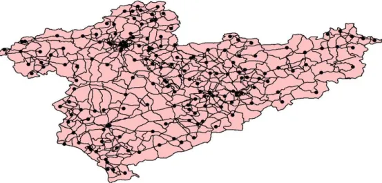
The suggested model is applied in the Central Anatolian Region of Turkey. There are 170 administrative districts in this region. It is first thought to apply the model on the national highway network with all of the mentioned 170 administrative districts. A detailed highway network data of Turkey is bought from the İşlem GIS firm in Ankara, Turkey. (Figure 4.1) The obtained highway network is processed with the GIS software ArcView 3.1 and it is observed that in addition to the 170 districts there are about 360 node junctions which make a total of 530 nodes in the Central Anatolian Region.
CHAPTER 4 APPLICATION IN TURKEY
30 As it is mentioned in Chapter 2 most of the papers in the hazardous waste location-routing literature presents applications with small instances, such as with 10 or 15 node networks. Even though we presented a somewhat more realistic model than the other models presented in the literature; there is no need for such a crowded network with 530 nodes. We would like to track our model using optimization software, and we believe that this would be hard with a 530 node network. We would also like to know if our model is solvable in reasonable CPU times.
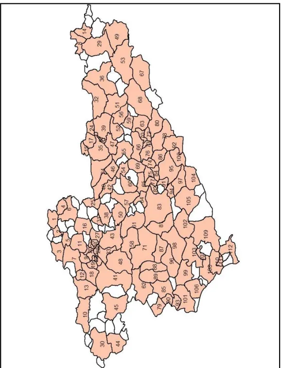
Thus we proposed obtaining another network in the Central Anatolian Region. We decided to include the districts with a population of more than 20000 in the region which makes a total of 112 administrative districts. Then the shortest paths are calculated with a simple script (code) written in GIS software ArcView 3.1 among all of the 112 districts on the national highway network. This new generated complete network is consisted of 112 nodes which correspond to 112 administrative districts of the region. The nodes of this generated network can be seen in Figure 4.2. The locations of the nodes on this network are the population centers of the administrative districts which are obtained from the GIS data that is bought from the İşlem GIS firm.
Figure 4.2 Selected 112 districts of the Central Anatolian Region All of the 112 nodes generate hazardous wastes. The data on the amount of hazardous wastes produced by each district in Turkey has not yet been prepared by the State Statistics Institute, but is planned to be ready in about a year. So the amounts of hazardous wastes generated by the districts are assumed to be directly proportional to the population of the districts.
At first 15 candidate nodes are selected for the location of both treatment and disposal centers. Those 15 candidate nodes are among the generation nodes (as all nodes generate hazardous wastes), and both treatment and disposal facilities are allowed to be located at the same node. Then, a 20 node candidate set is obtained by adding 5 new nodes to the previous 15 candidate set.
CHAPTER 4 APPLICATION IN TURKEY
32 Another important issue is how to determine the candidate sites. In real life, the candidate sites are determined by the related authorities, which are Ministry of Environment and municipalities for Turkey. For our case, the decision makers who decide on the candidate set would be ourselves. There are 13 provinces in the Central Anatolian Region. One candidate among each of the provinces is selected which makes up 13 candidate sites. One candidate is added to the provinces with higher populations, which are Ankara and Kayseri. Selecting the candidate administrative district among the provinces is done by subjective judgment. Also in determining the 20 node candidate set we again added one district to the candidate set from each province with relatively higher populations.
Three types of hazardous wastes are generated. The first type is composed of the hazardous wastes that can be incinerated, the second type is composed of the hazardous wastes that are not suitable for incineration but suitable only for chemical treatment, and the third type is both suitable for incineration and chemical treatment.
We suggested opening two treatment technologies. First technology is the incineration and the second technology is the chemical treatment. The first type of hazardous wastes, which are composed of the wastes that can be incinerated, is compatible with incineration and not compatible with chemical treatment. Whereas, the second type of hazardous wastes is compatible with chemical treatment and not compatible with incineration. Lastly, the third type of hazardous wastes is compatible both with the incineration and the chemical treatment technologies.
Distances are used as a measure of cost. Costs of transporting waste residues are taken 30% less than the costs of transporting hazardous wastes as
hazardous wastes are transported with special care such as with special trucks, and special equipment. The fixed annual cost for treatment centers is estimated by taking the annual costs of treatment centers in Turkey into account.
The population exposure band-width is taken as 800 meters for all types of hazardous wastes. The population exposure data is calculated via GIS. A script is written in the GIS software ArcView 3.1 which calculates the number of people in the band-width of 800 meters within the shortest path from one district to another. It is assumed that the population is uniformly distributed within the administrative districts. While solving the model to minimize risk, to avoid locating the disposal centers too far from the treatment centers a scaled “risk” value is implemented into the model for the waste residues. For the recycling issues, recycling after generation is not adopted. This is because hazardous wastes may not always be suitable for recycling. However, 30% of recycling is assumed after chemical treatment, which means 30% of the waste residues produced after chemical treatment is not sent to disposal centers but recycled. The waste residues after incineration are only composed of ashes which are not suitable for recycling.
Chemical treatment is a process in which the aim is only to reduce the hazard characteristics of the wastes not to reduce volume or mass. On the other hand, incineration is a process with high mass and volume reduction. Thus, the mass reduction in the incineration is taken as 80%, whereas the mass reduction after chemical treatment is taken as 20%. [5]
With this given network and parameters the problem is solved firstly by minimizing cost and then by minimizing risk using CPLEX version 8.1. We varied the minimum amount of waste to be processed at two of the given
CHAPTER 4 APPLICATION IN TURKEY
34 treatment technologies and the number of disposal centers to be opened. By varying the minimum amount of waste to be processed at the treatment technologies the model decides on the number of treatment centers to be opened. Even though there exists a fixed annual cost of opening a treatment technology in the cost objective; it is hard to predict the value of this fixed cost parameter. Thus, instead of varying the fixed cost we varied the minimum amount of waste to be processed at the treatment technologies in determining the number of treatment centers to be opened.
We considered three cases: Case 1 is when the minimum amount required for the incinerator is taken as 6000 units, for the chemical treatment it is taken as 4000 units and number of disposal centers to be opened is 1, case 2 is when the minimum amount required for the incinerator is taken as 3000 units, for chemical treatment it is taken as 2500 units and the number of disposal centers to be opened is 1, and case 3 is when the minimum amount required for the incinerator is taken as 3000 units, for chemical treatment it is taken as 2500 units and the number of disposal centers to be opened is 2. (Table 4.1) Case 1 corresponds to opening one treatment center of each treatment technology and one disposal center, Case 2 corresponds to opening two treatment centers from each treatment technology and one disposal center and Case 3 corresponds to opening two treatment centers from each treatment technology and two disposal centers. Minimum amount required for incinerator Minimum amount required for chemical treatment Number of disposal centers to be opened Case 1 6000 4000 1 Case 2 3000 2500 1 Case 3 3000 2500 2
The problem is solved with the given parameters (Case 1, 2 and 3) by using the given linear composite scalarized objective function and by varying the weights given to λ.
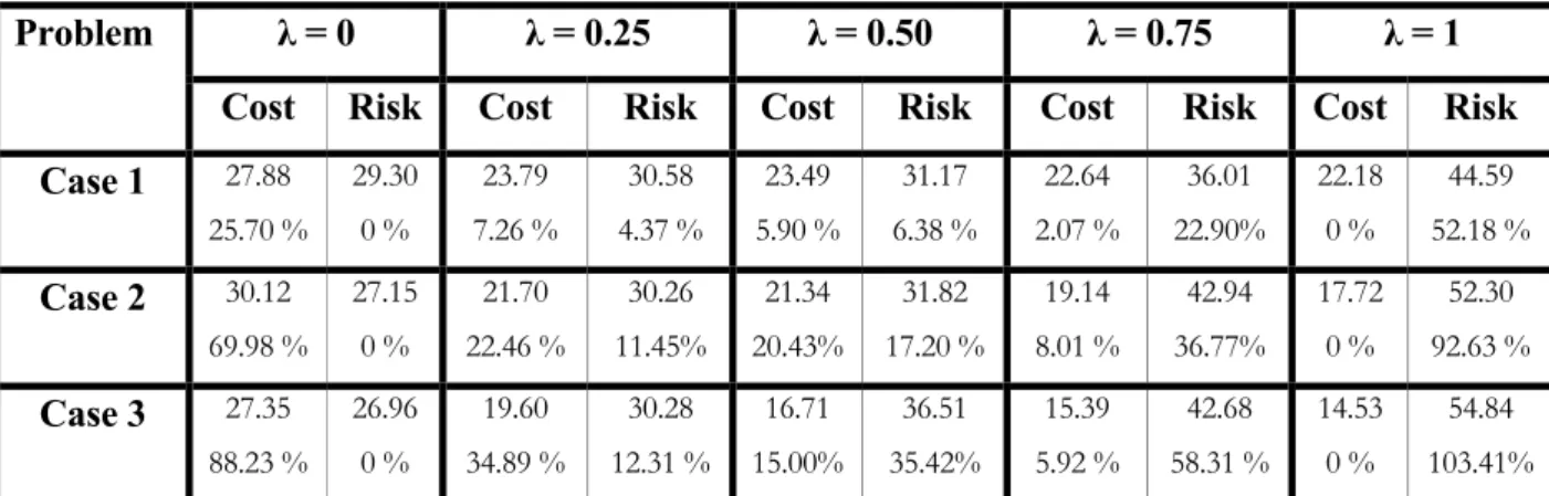
The results for the 15 candidate solution are summarized in Table 4.2 for both minimum cost and minimum risk solutions in all of the three cases.
Problem Cost (ton-km) Risk (ton-people) Incinerator Chemical treatment Disposal Center 22.18 44.59 Kaman Kaman Kaman Case 1
27.88 29.30 Kaman Kaman Kaman
17.72 52.30 Altındağ, Avanos Altındağ, Kaman Keskin Case 2 30.12 27.15 Ilgaz, Kaman Sivrihisar, Avanos Kaman 14.53 54.84 Altındağ, Avanos Altındağ, Avanos Altındağ, Avanos Case 3 27.35 26.96 Ilgaz, Kaman Sivrihisar, Avanos Sivrihisar, Avanos Table 4.2 Minimum cost and minimum risk solutions for 15 candidates In case 1, both minimum cost and minimum risk solutions place all treatment technologies and the disposal center to Kaman, which a district of the province Kırşehir. Kaman is selected as it is located in the center of the region and the transportation routes leading to Kaman are among the least populated routes (Appendix-1). Even though both of the treatment centers and the disposal
CHAPTER 4 APPLICATION IN TURKEY
36 center are located in Kaman in all minimum cost, minimum risk solutions and the solutions with the linear combination of cost and risk (Table 4.3), the routing strategies are different.
Problem Case 1 Case 2 Case 3
Incinerator Plant
Kaman Ilgaz, Kaman Ilgaz, Kaman Chemical
Treatment
Kaman Sivrihisar, Avanos Sivrihisar, Avanos λ = 0
Disposal Center
Kaman Kaman Sivrihisar, Avanos
Incinerator Plant
Kaman Sincan, Kaman Sincan, Avanos Chemical
Treatment
Kaman Keskin, Avanos Keskin, Avanos λ = 0.25
Disposal Center
Kaman Keskin Keskin, Avanos
Incinerator Plant
Kaman Sincan, Avanos Altındağ, Avanos Chemical
Treatment
Kaman Keskin, Avanos Sincan, Avanos λ = 0.50
Disposal Center
Kaman Keskin Sincan, Avanos
Incinerator Plant
Kaman Sincan, Avanos Sincan, Avanos Chemical
Treatment
Kaman Altındağ, Avanos Altındağ, Avanos λ = 0.75
Disposal Center
Kaman Avanos Altındağ, Avanos Incinerator
Plant
Kaman Altındağ, Avanos Altındağ, Avanos Chemical
Treatment
Kaman Altındağ, Kaman Altındağ, Avanos λ = 1
Disposal Center
Kaman Keskin Altındağ, Avanos Table 4.3 Treatment and disposal centers’ locations with 15 candidate sites
If one wants to locate one treatment and disposal center in the Central Anatolian Region (Case 1) with those 15 candidates, both centers will be located in Kaman without considering the objectives. However, in determining the allocated routes of the generation centers one should chose the best compromising solution among the resulted routing strategies. In Case 2 and Case 3, it is observed that different locations are selected such as Avanos, Ilgaz, Altındağ, Sincan and Sivrihisar. (Table 4.3)
Table 4.3 summarizes the selected locations of treatment technologies and disposal centers for the 15 candidate solution in all of the three cases. The given districts and the locations of these districts in the region can be seen in Apendix-1. Almost all of the selected districts in the solutions are located around the most populated provinces in the Central Anatolian Region as the amount of generated hazardous wastes are assumed to be proportional with the population of the districts.
Table 4.4 summarizes the results obtained with the weights given to λ. It also presents the deviations from the minimum for both cost and risk values. Percent deviation from the minimum is calculated as follows:
CHAPTER 4 APPLICATION IN TURKEY
38
λ = 0 λ = 0.25 λ = 0.50 λ = 0.75 λ = 1
Problem
Cost Risk Cost Risk Cost Risk Cost Risk Cost Risk Case 1 27.88 25.70 % 29.30 0 % 23.79 7.26 % 30.58 4.37 % 23.49 5.90 % 31.17 6.38 % 22.64 2.07 % 36.01 22.90% 22.18 0 % 44.59 52.18 % Case 2 30.12 69.98 % 27.15 0 % 21.70 22.46 % 30.26 11.45% 21.34 20.43% 31.82 17.20 % 19.14 8.01 % 42.94 36.77% 17.72 0 % 52.30 92.63 % Case 3 27.35 88.23 % 26.96 0 % 19.60 34.89 % 30.28 12.31 % 16.71 15.00% 36.51 35.42% 15.39 5.92 % 42.68 58.31 % 14.53 0 % 54.84 103.41%
Table 4.4 Cost and risk values for given linear combinations and deviations from the minimum for 15 candidates.
For case 1, the solutions with λ = 0.25 and λ = 0.50 seems to be better choices, as the percent deviations from the minimum for both cost and risk in both of the solutions are less than 10%. For case 2, λ = 0.25 solution would be a better choice with a lower risk value and a little higher cost value than that of λ = 0.50 solution. For case 3, again λ = 0.25 solution seems to be better. However, one should keep in mind that the best solution may differ for every decision maker. In this application decision maker is the author, whereas in the real case the decision makers would probably be the government, for Turkey the decision maker is the Ministry of Environment.
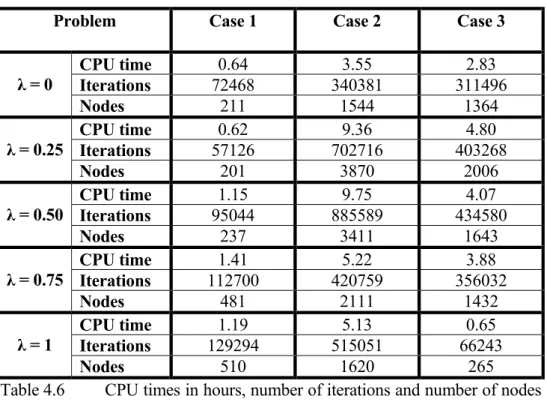
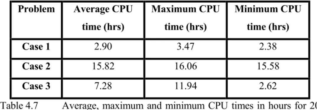
The problem is solved in reasonable CPU times, where the fastest result is obtained in about 40 minutes and the longest result took about 10 hours with 15 candidates. Table 4.5 presents the average, maximum and minimum CPU times obtained in all of the three cases with 15 candidates. Table 4.6 summarizes the CPU times, number of iterations and number of nodes obtained in the 15 candidate solutions using CPLEX Version 8.1.
Problem Average CPU time (hrs) Maximum CPU time (hrs) Minimum CPU time (hrs) Case 1 1.00 1.41 0.62 Case 2 6.60 9.75 3.55 Case 3 3.24 4.80 0.65
Table 4.5 Average, maximum and minimum CPU times in hours for 15 candidate solutions
Problem Case 1 Case 2 Case 3
CPU time 0.64 3.55 2.83 Iterations 72468 340381 311496 λ = 0 Nodes 211 1544 1364 CPU time 0.62 9.36 4.80 Iterations 57126 702716 403268 λ = 0.25 Nodes 201 3870 2006 CPU time 1.15 9.75 4.07 Iterations 95044 885589 434580 λ = 0.50 Nodes 237 3411 1643 CPU time 1.41 5.22 3.88 Iterations 112700 420759 356032 λ = 0.75 Nodes 481 2111 1432 CPU time 1.19 5.13 0.65 Iterations 129294 515051 66243 λ = 1 Nodes 510 1620 265
Table 4.6 CPU times in hours, number of iterations and number of nodes of 15 candidate solutions
The results obtained with 20 candidates turned out to be the same, in terms of treatment and disposal center locations and routing strategies, that are obtained with 15 candidates. This means that the addition of 5 new candidate sites did not make any difference in solutions except in CPU times. We would like to know how the CPU time is effected when the candidate set is enlarged. Thus
CHAPTER 4 APPLICATION IN TURKEY
40 we provide Table 4.7 which shows the average, minimum and maximum CPU times obtained while solving the model with 20 candidates in all of the three cases. The tables (Table 4.2, 4.3, 4.4) which show the solutions of the 15 candidate problem are valid for the 20 candidate solutions.
Problem Average CPU time (hrs) Maximum CPU time (hrs) Minimum CPU time (hrs) Case 1 2.90 3.47 2.38 Case 2 15.82 16.06 15.58 Case 3 7.28 11.94 2.62
Table 4.7 Average, maximum and minimum CPU times in hours for 20 candidate solutions
When we compare the CPU times obtained in 15 candidate solutions with 20 candidate solutions, we observed that the CPU times for Case 1 is not much affected. The maximum increase is observed in Case 2, where the average CPU time with 15 candidate sites is 6.60 and the average CPU time with 20 candidate sites is 15.82. Again in Case 3, even there is about a 4 hours increase in average CPU times with 20 candidate solutions compared to 15 candidate solutions the increase is less than the increase observed in Case 2.
20 25 30 35 40 45 50 20 22 24 26 28 30 Cost Ri sk
Figure 4.3 Trade-off curve
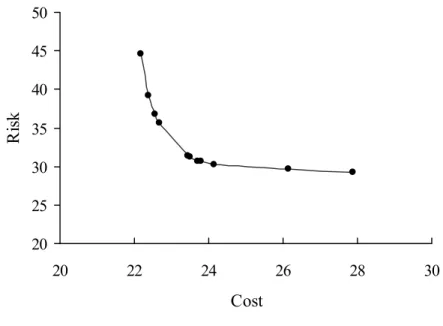
Lastly, a trade-off curve is drawn for Case 1 with 15 candidates where the model locates one treatment center of each treatment technology and one disposal center. (Figure 4.3) We varied λ between 0 and 1 by an increment of 0.1 each time. We observed that there is a steep increase in cost when λ = 0, and there is a steep increase in risk when λ= 1. Thus minimum cost and minimum risk solutions may not be suitable for implementation, as for example if minimum cost solution is adopted then the corresponding risk value will be too high. From the trade-off curve it seems to be more reasonable to implement a solution with the λ value being between 0.6 and 0.2.
42
C h a p t e r 5
CONCLUSIONS AND FUTURE
RESEARCH DIRECTIONS
The hazardous waste management problem is an important problem which should be handled with special care. Hazardous waste management is differentiated from the casual waste management problems as hazardous wastes may threat human health, welfare and environment.
As we observed the hazardous waste management literature we have seen that the proposed models do not reflect the real life situations. Various assumptions are made in the presented models which lead to simplified, not applicable models in real life. Thus, we believe that the hazardous waste management literature lacks a mathematical model reflecting many of the real life aspects of the problem which can be implemented to real life problems.
We proposed a new mixed integer programming model in which we combined the applicable aspects from different models in the literature. Our model also includes the constraints that reflect certain requirements that have been observed in the literature but could not been incorporated into the models correctly, together with the additional constraints that we propose. The aim of the model is to decide on the following questions: where to open treatment centers with which technologies, where to open disposal centers,