Hard spin mean field theory of 3D stacked-triangular-lattice system

Q C

, р п Ä "it І Э Э t |

c.

Í

'P : } p f /β,Μ_{# « Ч W· ■ Ф '« .w·;·· '-é\^} ΐ.ί" ■' ',' · ■ ~νΤ · /*Ѵ / ^ r^i ■' '¡^ '' ■ ' \φ,' «■ y · ■ »-^ ’* !^·^ f' * Ρ Λ '*^-:·' ' ·^ * * ' ; Γ'» ¿ík m. .«МММ. «*· 4¡,r·

HARD SPIN MEAN FIELD THEORY OF 3D

STACKED-TRIANGULAR-LATTICE SYSTEM

A THESIS

SUBMITTED TO THE DEPARTMENT OF PHYSICS AND THE INSTITUTE OF ENGINEERING AND SCIENCE

OF BILKENT UNIVERSITY

IN PARTIAL FULFILLMENT OF THE REQUIREMENTS FOR THE DEGREE OF

MASTER OF SCIENCE

By

Giirsoy Bozkurt Akgiig

June 1, 1994

I certify that I have read this thesis and that in my opinion it is fully adequate, in scope and in quality, as a dissertation for the degree of Master of Science.

Prof. Dr. Cemal Yalabık (Supervisor)

I certify that I have read this thesis and that in my opinion it is fully adequate, in scope and in quality, as a dissertation for the degree of Master of Science.

Prof. Dr. A. Shumovsky

I certify that I have read this thesis and that in my opinion it is fully adequate, in scope and in quality, as a dissertation for the degree of Master of Science.

b j C

і е э ц

Ill

Approved for the Institute of Engineering and Science:

Prof. Mehmet Baray, / y

Abstract

HARD SPIN MEAN FIELD THEORY OF 3D

STACKED-TRIANGULAR-LATTICE SYSTEM

Giirsoy Bozkurt Akgiig

M.S. in Physics

Supervisor: Prof. Dr. Cemal Ycilabik

June 1, 1994

Closed form solution of ‘Hard spin mean field theory’ is constructed

and applied to ‘Three dimensional stacked-triangular-system’. The phase

diagram of this system is examined. ‘Free energy’ is calculated to reveal the thermodynamically stable state in the phase diagram. A new second order phase transition line is found near the zero external magnetic field. Strong evidence is found for the tricriticality point behaviour in the multicritical region.

özet

3 BOYUTTA SIRALANMIŞ ÜÇGEN ÖRGÜSÜNÜN SABİT

SPİNLİ ORTALAMA ALAN TEORİSİ

Gürsoy Bozkıırt Akgüç

Fizik Bölümü Yüksek Lisans

Tez Yöneticisi: Prof. Dr. Cemal Yalabık

1 Haziran 1994

‘Sabit spinli alan kuramının’ kapalı durumdaki çözümü yapıldı ve ‘üç boyutta sıralanmıs-üçgen-örgülü sisteme’ uygulandı. Bu sistemin faz diyagramı incelendi. ‘Serbest enerji’ hesaplanarak, termodinamik açıdan dengede olan durumlar faz diyagramında gösterildi. Yeni bir ikinci dereceden faz geçiş çizgisi bulundu. Çoklukritik bölgenin bir üçlükritik nokta davranışı gösterdiğine dair güçlü kanıtlar bulundu.

Acknowledgement

I would like to thank to Prof. Dr. C. Yalabık for his supervision, guidance and suggestions through the development of this thesis.

I would also like to thank to Prof. Dr. A. Shumovsky and Assoc. Prof. Dr. B. Tanatar for reading and commenting on the thesis.

It is a pleasure to express my thanks to all my friends for their valuable discussions and assistance.

Contents

A bstract ₁₁₁

Ozet

A cknow ledgem ent Vll

1 IN T R O D U C T IO N

2 H A R D S P IN M E A N FIELD TH EO RY

2.1 MEAN FIELD TH EORY... 3 2.1.1 Mean field theory of the Ising M o d e l ... 4 2.1.2 Critical point of view for the conventional mean field theory 7

2.2 LANDAU - GINZBURG MEAN FIELD THEORY 9

2.3 HARD SPIN MEAN FIELD THEORY 10

3 FR U ST R A T E D SY STEM S 12

3.1 GENERAL PROPERTIES OF THE ISING M A G N E T ... 12

CONT EN TS _IX 3.1.1 Spontaneous Symmetry B re a k in g ... 17 3.1.2 Broken Ergodicity... 19 3.2 FRUSTRATION 19 3.3 MULTICRITICAL P O IN T S ... 21 4 A N A PPL IC A T IO N TO FR U ST R A T E D SYSTEM S 23

4.1 SYSTEM, MODEL AND THE M E T H O D ... 23

4.1.1 Hard Spin Mean Field Theory: Formulation of the Problem 24

4.1.2 Solution of the Coupled Equations 26

4.2 PHASE DIAGRAM... 27 4.2.1 Free Energy C a lc u la tio n s ... 32

List of Tables

List of Figures

3.1 Phase transition and critical phenomena in magnetic systems . . 14 3.2 Free energy density for finite and infinite s y s te m ... 19 3.3 Frustration. Example 1... 20

3.4 Frustration. Example 2. 21

3.5 multicritical p o i n t s ... 22

4.1 Hard spin mean field formulation in triangular l a t t i c e ... 26 4.2 The phase diagram of the ‘Three dimensional

stacked-triangular-lattice system’... 28 4.3 Sublattice magnetizations for T = 3: first order phase transition 29 4.4 Sublattice magnetizations for different temperatures:second

order phase transition . ... 30 4.5 Sublattice magnetizations for no external magnetic fie ld ... 32 4.6 Free energy of two phases in the zero external magnetic field. . . 33 4.7 Free energy of two phases for T = 3... 34

Chapter 1

INTRODUCTION

Phase diagram of a system defines its ordered states (i.e. phases, which have different thermodynamic properties) and what type transitions occur between them. The knowledge of the phase diagram in detail is important both from an application point of view and also as an academic interest. Different phases of a system correspond to different values of the corresponding order parameters. (Some examples of order parameters are the density in fluids, magnetization in magnetic systems, polarizability in the ferroelectrics etc.) These phases are separated from one another with phase boundaries and phase transitions occur between different phases at these points.

There are various methods for examining the phase diagram. Some of these are mean field theory, renormalization group theory or Monte Carlo simulations. In this work, ‘hard spin mean field theory’ is used in the examination of the phase diagram of the ‘3D stacked-Triangular-Lattice system’ which is a frustrated system. Hard spin mean field theory is a recently developed method which is especially successful in application to a frustrated system.

In previous works, Monte Carlo implementation of ‘hard spin mean field theory’ was done. The error bound did not allow a detailed picture of the phase diagram especially in the region of which external magnetic field is

Chap ter 1. INTROD UCTION

close to zero. In this work, the closed form of the corresponding hard spin mean field equations is developed and applied to the ‘3D stacked triangular lattice systems’. Various aspects of the the phase diagram is examined. A new phase boundary is found near zero nicignetic field. The characteristic of the multicritical region is evident from the calculations.

In the second chapter, a brief introduction to the method used in the examination of the phase diagram is given. Mean field theory and Hard spin mean field theory is explained. In chapter 3, the concepts of frustration and frustrated system are described. In the last part of this chapter, we give some information about the multicritical points which is relevant to the system under consideration. In chapter 4, application of hard spin mean field theory to the stacked triangular lattice antiferromagnetic systems is described in detail. Last chapter presents the conclusions of the work.

Chapter 1

INTRODUCTION

Phase diagram of a system defines its ordered states (i.e. phases, which have different thermodynamic properties) and what type transitions occur between them. The knowledge of the phase diagram in detail is important both from an application point of view and also as an academic interest. Different phases of a system correspond to different values of the corresponding order parameters. (Some examples of order parameters are the density in fluids, magnetization in magnetic systems, polarizability in the ferroelectries etc.) These phases are separated from one another with phase boundaries and phase transitions occur between different phases at these points.

There are various methods for examining the phase diagram. Some of these are mean field theory, renormalization group theory or Monte Carlo simulations. In this work, ‘hard spin mean field theory’ is used in the examination of the phase diagram of the ‘3D stacked-Triangular-Lattice system’ which is a frustrated system. Hard spin mean field theory is a recently developed method which is especially successful in application to a frustrated system.

In previous works, Monte Carlo implementation of ‘hard spin mean field theory’ was done. The error bound did not allow a detailed picture of the phase diagram especially in the region of which external magnetic field is

Chapter 1. INTRODUCTION

close to zero. In this work, the closed form of the corresponding hard spin mean field equations is developed and applied to the ‘3D stacked triangular lattice systems’. Various aspects of the the phase diagram is examined. A new phase boundary is found near zero magnetic field. The characteristic of the multicritical region is evident from the calculations.

In the second chapter, a brief introduction to the method used in the examination of the phase diagram is given. Mean field theory and Hard spin mean field theory is explained. In chapter 3, the concepts of frustration and frustrated system are described. In the last part of this chapter, we give some information about the multicritical points which is relevant to the system under consideration. In chapter 4, application of hard spin mean field theory to the stacked triangular lattice antiferromagnetic systems is described in detail. Last chapter presents the conclusions of the work.

Chapter 2

HARD SPIN MEAN FIELD

THEORY

Mean field theory provides a useful starting point for analysis of models for phase transition. Although it may not give very accurate quantitative details, one usually can obtain a very good insight into the problem, the symmetries, various phases, etc. Based on this knowledge, one may then go on to the use of analytical techniques, renormalization group calculations, Monte Carlo simulation and other combined methods. Due to its simplicity, the mean field approach is a helpful method to understand the problem and the result of proceeding analysis.

2.1

MEAN FIELD THEORY

Historically, conventional mean field theory was formulated by P.E.Weiss as a theory of magnetism. It was the only theory of phase transition for a long time. Later, an argument due to L.D.Landau suggested that mean field theory was essentially exact. We now know that this is not the case, except for sufficiently large values of the spatial dimensionality or for infinite-range interactions. For a historical discussion see the Nobel lecture of K. G. Wilson.*

Chapter 2. HARD SPIN MEAN FIELD THEORY

The term mean field theory conveys an impression of uniqueness but there are many ways to generate mean field theories and various systems and models on which mean field theory can be applied. Therefore we restrict ourselves to the excimination of the Hard spin mean field theory of the simple Ising modeH in magnetic systems.

2.1.1

M ean field th eo ry o f th e Isin g M o d el

One of the simplest models of a magnetic system is the Ising Model which is capable of describing the phase transition of the system. It was proposed for the ferromagnetic - paramagnetic phase transition initially, but later it was applied to a variety of problems of different nature. The model is defined on a lattice with a symmetry and dimensionality appropriate to the system to be modeled. Each lattice point is associated with a number 5, which can take the values ±1. Here Si is called the quasi spin and it defines, for instance, a domain of localized electrons with a total magnetic moment in the units of Bohr magneton in atomic units. The system Hamiltonian is

Hi.sing (2.1)

where the sum over i and k runs over all possible nearest-neighbor pairs of the lattice. J is the exchange coupling which can be derived from the overlap integral of electron wave function, and, its sign results in the ferromagnetic or antiferromagnetic property of the magnetic system. The variable h represents the external magnetic field exerted on the system.

The partition function for the Ising model can now be written as

■Rising — (2.2)

where ^ = l / k s T is the inverse temperature, /cg is the Boltzman constant, and if taken as unity, temperature T may be expressed in energy units. In all definitions, the summation is carried out over all possible values of the spins. For N spins this implies E{5} = EsuS2,-Sn ■

Chapter 2. HARD SPIN MEAN FIELD THEORY

The relation of Z to thermodynamics is the main axiom in statistical mechanics, and is generally applicable to any system:

Z ls in g = e x p i - / ? / · ) =

_(2.··!)

where F is the free energy of the system. All thermodynamic quantities of the system can be derived from the knowledge of it. (See table 1 in Chapter 3.)

Averaging of any thermodynamic quantity, for instance, the spin, is given by

(‘5’.·) = ^fsing · · (2.4)

De r i v a t i o n o f t h e c o n v e n t i o n a l m e a n f i e l d e q u a t i o n s

Equation 2.4 can be put in a more convenient form so that mean field equations may be derived easily. For this purpose, the configurational sum is split into two parts, {5} — >■ {5, 5';} where S denotes the set of all ¿"’s except a particular 5',·. ^ E{5} e x p ( - № ,in g [ 5 ]) ^ , о TT r o u E ^. = ±lMi-exp(-/3Hisi„g[Mi,S]) E { 5 } e x p ( - ^ Я I s ¡ n g h ) · E { 5 } e x p ( - / ^ ^ i s i n g [ 5 ’]) (2.5)

If the summation is taken over Si , we get exp( — 5]) which

exactly cancels the term E^.=±i exp(—/9//[^i,·, 5]). The remaining term in the numerator, E {5},,t,=±i e x p (- ^ if [ /q ,.?]) becomes, J2{s}Si ■ e x p [- /3H{S)] when p is renamed S{.

On the other hand, if the summation is carried out over possible values of

p ( — ± 1), we obtain

^ E{s}exp(-/^-^Isiiig['3'])tanh(^hj + f^ZkJjkSk)

E{s}exp(-/?iilsmg['5])

It is customary to call the argument of the hyperbolic tangent function as effective field, = hj +

Eqn. 2.6 shows that the expectation value of the spin Si is exactly equal to the expectation value of the hyperbolic tangent of the effective field h^^acting on it.

If we approximate the average in Eqn. 2.6 such that all appearances of S\ inside the average are replaced by their average values (Sk)·,

(Si) = rui = (tanh(^h,· + pJu-Si,))

« tanh(y5hj· + PJiki^k) (2-7)

This is the conventional mean field approximation for the Ising Model.

There are different ways to construct the mean field approximation other than the one above. The general procedures will be stated here, instead of explicit derivations: (It is possible to find the detailed results in the book of Binney et. al.^)

Chapter 2. HARD SPIN MEAN FIELD THEORY 6

• Expectation values of products of the form {Si · Sk) may be approximated as (Si) ■ {Sk)· In other words, interaction of Si with all other spin is replaced by the interaction of Si with a local magnetic field, h^ff, produced by all other spins. (The fluctuations in the system are ignored.) • Instead of the actual interaction of S) with its nearest neighbor spins, it

is assumed that Si interacts equally with all the spins in the system, {i.e. long range order is more likely than short range order.) However the coupling constant must be modified with a normalization factor which is proportional to the system size, J —> JJN where N is the number of spins in the system. (A special case of this assumption is known as Bragg-Williams approximation for the model of an alloy system.^) • • The minimization of the free energy using the Boltzman distribution in

a restricted set of probability measures, an approximate solution can be obtained. If product measures (i.e. measures in which the spins are statistically independent) is used, mean field theory can be obtained. (This is called the variational approach.)

Chapter 2. HARD SPIN MEAN FIELD THEORY

• Mean field theory Ccin also be obtained from the zeroth order approxima­ tion of perturbation expansion ciround the Gaussian Model.

• Saddle Point approximation in the Landau Ginzburg Hamiltonian gives mean field results.

So l v i n g t h e m e a n f i e l d Eq u a t i o n

The procedure for finding the magnetization can be understood easily by considering the above statements of the mean field approximation. Each spin experiences the presence of an effective field hgff due to the magnetic moments of all of the other spins. These magnetic moments would be proportional to the magnetic moment M of all the other spins, which is itself unknown a priori. Thus a given spin experiences both the externally applied field and the effective field due to the other spins. The combination of the two fields then determines the response of the given spin, ¿.e., its average magnetic moment. But there is nothing special about this chosen spin, therefore its moment must be the average magnetic moment M . In this way, M is calculated self consistently.

2.1.2

C ritica l p o in t o f v ie w for th e co n v en tio n a l m ean

field th e o r y

It is necessary to understand some methodical problems of the theory before interpreting its results. This is also useful for choosing which system or model to study as a problem for which mean field theory would be expected to give good results.

Some weak points of the theory are introduced first:

• Short range forces are oversimplified in the treatment of conventional mean field theory. In this way mean field analysis gives immediately non zero magnetization below some fixed temperature without external magnetic field as a result of broken symmetry. (This is the phase

Chapter 2. HARD SPIN MEAN FIELD THEORY

transition at this point.) The finite magnetization is the result of long range order in the system. In the case of conventional mean field theory, it is inevitable to obtain a phase transition even in a one dimensional system with short range interaction, for which it can easily be shown that a phase transition is strictly forbidden. (The generalized theorem ‘Long range order exist in system when dimension > 2’ is known as the Mermin-Wagner theorem.*^)

• Critical exponents predicted by mean field theory can easily be found by expanding the thermodynamic functions near the critical points. There are clearly systematic differences between these values and the

experimental ones. Mean field exponents do not depend on system

dimensionality whereas exact critical exponents do.

• Since fluctuations are removed from the system, critical temperature determined by mean held theory is always greater than the real critical temperature. Long-wavelenght fluctuations enable the system to enjoy almost all the energetic benefits of the ordered state without the entropy cost associated with macroscopic ordering.

• Mean field theory is not accurate near the transition point since fluctuations are removed. But fluctuation is infinite at the critical temperature.

On the other hand, some positive points of the theory are;

• The order parameter of the system is identified and described as simply as possible.

• It is possible to give a description of the metastable state of the system, which is difficult to obtain by other methods.

• Mean field theory exhibits universality although a wrong one, a feature that emerges from the general framework of Landau theory.

• Direct use of mean field theory calculations sometimes gives very good agreement with the experiment, the magnetic substance HoRh,iB4 being an example.^

Chapter 2. HARD SPIN MEAN FIELD THEORY

• It predicts the possible phase diagram which is not always true but

provides a good starting point for future analysis.

• Mean field theory is exact for the case of the infinite range interaction Ising model in which the exchange coupling has a finite value for all spin-spin interactions in the system.

The aim of other versions of the mean field theory is to find a reasonably good approximation (other than the conventional mean field theory) to the exact equation which is given by Eqn. 2.6.

2.2 LANDAU - GINZBURG MEAN FIELD

THEORY

The basic idea in this approach is to focus on the energetics of a slowly varying local order parameter configuration (such as the magnetization in Ferromagnetic system). Underlying discrete lattice structure of the material is ignoi'ed and it is described as a continuum. The local order parameter at position r is given functionally as r}{r).

Landau theory postulates that a local free-energy function L (known as Landau free energy) which depends on the coupling constants and the order parameter can be constructed.® L has the property that the state of the system is specified by the absolute minimum of L with respect to the order pariimeter.

L has dimension of energy but is not identical to Gibbs Free Fnergy.(For a

homogeneous system with volume V, Landau free energy density is defined as A = L IV .) To specify L it is sufficient to use the following constraints:

• Description of L has to be consistent with the symmetries of the system. • Near the critical temperature, L can be expanded in a power series in

Chapter 2. HARD SPIN MEAN FIELD THEORY ₁₀

• In a inhomogeneous system, L is a local function of the order parameter and it has a finite number of derivatives at a general point in space.

A for a homogeneous system in a magnetic field can be found by expanding the order parameter near the critical temperature:

A = ao + a2T]^' + a.pf - ht], (2.8)

where ao{J, ¡3),a2{Ji (3)·, a4{J, /1) ^re the expansion coefficients and the order

parameter t] is the magnetization. For an inhomogeneous system, square of

the first derivative of 77(r) is also added to L. This term governs the thermal fluctuation of the order parameter. It is impossible to get analytical results using the Landau-Ginzburg free energy functional for a general inhomogeneous system. It is necessary to carry out the saddle point approximation or Gaussian approximation. For a detailed study of Landau-Ginzburg theory see Ref..^

2.3 HARD SPIN MEAN FIELD THEORY

Hard spin mean field theory has been developed recently^ to improve upon the conventional mean field theory. It was first applied to frustrated systems by Netz and Berker,^® and self consistent equations were solved by a Monte Carlo implementation. Later, the method was applied to stacked triangular systems and iterative solution were o b ta in e d .T h e method is very successful in its application to frustrated systems.

In this approach, the effect of the full magnitude of each spin is taken into account. This condition is essential for application of the method to a frustrated system. This point will be discussed further in the next chapter- after an examination of frustrated systems.

The basic idea behind this method may be demonstrated through its application to the simple Ising model. Instead of using Eqn. 2.6 for- specifying the effective field acting on a spirr, one uses the full magnitude of the interacting spins, weighted with appropriate probabilities associated with those

Chapter 2. HARD SPIN MEAN FIELD THEORY ₁₁

magnitudes, i.e., the effective field is taken as m,· = tanh(/I(J2k’-^ikSk + h,)) where Sk = ± 1 with probability pk(S'k) = (1 + Skrnk)/2. The configurcitional sum is over all sites k that are coupled to i by the interaction Jik, and hj is the external field on Si. The compact formulation is

m ; = + hi)), (2.9)

where the sum {¿'fc} is over all interacting-neighbor combinations. The above is applicable to an arbitrary distribution of interactions and may be generalized to multispin interactions,^

m ; = t a n h ( / ? ( E . x , , , , ...+ ¡.¡))_klyk2y...,kn (2.10)

where Skj = ± 1 with probability pkjiSkj)·

This method is an improvement over the conventional mecin field theory in several respects:^^

• Due to the hard spin condition, antiferromagnetic and frustrated systems can be adequately described.

• It is easy to show that it is exact in one dimension for the Ising model in the absence of external magnetic field. •

• For comparison purposes, we note that in two dimensions the conven­ tional mean field theory gives f^cJ = 0.25 and the hard spin mean field theory gives ¡3cJ = .32.36 whereas the exact value is fScJ = 0.4407

Chapter 3

FRUSTRATED SYSTEMS

The concept of ‘frustration’ or competing interactions arise frequently in the examination of the ‘spin glass’ system which is a fascinating topic in condensed m atter physicsd^ A spin glass is a collection of spins (he. magnetic moments) in which the low-temperature state is frozen and disordered, in contrast to the uniform or periodically ordered ground state of the con\ entional magnetic system. It appears that in order to produce such a state there must be competition among the different interactions between the moments (i.e. no single configuration of the spins is uniquely favored by all the interactions).

3.1

GENERAL PROPERTIES OF THE

ISING MAGNET

The general approach for examining a magnetic system (as other problems of statistical physics) starts with a model of the system. This model must describe the real interactions of the system in a solvable simple form. After using a model Hamiltonian , thermodynamic properties of the system may be

determined through the free energy in the thermodynamic limit, h) =

liniA/^oo ^ ■ log(ZAf(^, h)).

Chapter 3. FRUSTRATED SYSTEMS ₁₃

As described earlier, Ising model''^ is the simplest model that can be used for magnetic systems. Now, the ferromagnetic properties of this model will be described. The Ising Hamiltonian with a positive coupling constant represents a ferromagnetic system.

Hn = - SiS'h - ^ hiSi

ik

(3.1) where J > 0. This sign results in a reduction of the interaction energy between neighboring spins when these spins point in same direction.

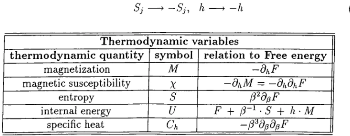
If the free energy of the system is known, all thermodynamic quantities of the system can be calculated from the relations given in the Table 3.1. Here h and ¡3 are the thermodynamic parameters (degrees of freedom) of the system and correspond to the magnetic field and the temperature in the ferromagnetic system. Free energy is therefore sufficient to describe the full thermodynamics of the system.

A finite magnetization without an external field corresponds to the ferro­ magnetic state and therefore magnetization is chosen as the order parameter. The dependence of magnetization on the thermodynamic parameters is shown in Fig 3.1.

The microscopic symmetries of the Hamiltonian can be used to understand the thermodynamic functions of the system. Hamiltonian in Eqn. 3.1 satisfies the following symmetry:

h -h (3.2)

Therm odynam ic variables

th erm od yn am ic quantity sym bol relation to Free energy

magnetization M - d h F

magnetic susceptibility _X - d h M = -dhdhF

entropy

s

!^‘% F

internal energy

u

F F 1 3 - Y S + h · M

specific heat c \ - f d g d g F

Chc^pter 3. FRUSTRATED SYSTEA4S ₁₄

a)

first order phase transition

y — critical point

---

O---c)

Figure 3.1: Phase transition and critical phenomena in magnetic systems

. a) Phase diagram, b) Magnetization M as a function of h. c) Spontaneous magnetization as a function of temperature

or

H

n

[I

i

,J,S

j

] = HM[-h,J,-Sj].

(3.3)

This is also known as time reversal symmetry or Z2 symmetry. As a result

of this symmetry it is easy to see why phase transition occurs when there is no external magnetic field (the proof is due to Lee and Yang^'*).

In Fig 3.1.a, for 0 < T < Tc the system exhibits a magnetization M in the absence of an applied field which can be either positive or negative. This is

Chapter 3. FRUSTRATED SYSTEMS ₁₅

called the ‘spontaneous magnetization’.

Symmetry of the Ising model is important for understanding the properties of the free energy function. Any function which results from a sum over all spin configurations satisfies spin inversion symmetry. This can be seen by inspection: since spin configuration takes both positive and negative values, which one it takes first does not matter. Therefore for any function $ of spins {,5',}, the configuration sum of does not change with changing sign of the spin:

E « ( ( 5 . ) ) = E 4’({-y.})· (3.4)

{s.=±l)

{5i=±l}

The symmetry properties given above lead to a free energy density which is an even function of the spin variable. The partition function can be shown to be symmetric with respect to the inversion of coupling constant as follows

Z

n

{-K J ,T )= ^ exp[-l3HM{-KJ,{Si])]

{ Si =±l } - e x p [ - № ( - A , J , {-,?.·})] {5i=±l} = Yj exp[-^/f/v(A ,J, {.S;·})]

{5.=±1}

= Zn{ K J , T ) . (3.5)

This implies free energy density is an even function of h.

by 3.4 by 3.2

SUB-LATTICE SYMMETRY OF ISING MODEL

Sub-lattice symmetry occurs when there is no magnetic field in the Ising model. One may divide the hypercubic lattice into two sublattices, say sublattices A and B. In the Hamiltonian

<ij>

Chapter 3. FRUSTRATED SYSTEMS ₁₆

the spins on sub-lattice A interact only with spin in sublattice B and vice versa. Therefore,

= - J E S f S f . (3.7)

<ij>

Hamiltonian in Equation 3.6 exhibits the symmetry - J , {5,^ - 5 f ))

(3.8)

W hat is the implication of this symmetry for the thermodynamics of the system? To answer this question it is necessary to find the effect of symmetries on the free energy density.

Z i v { 0 , - J , T ) = ^ e x p ( - ^ // y v ( 0, - J , T ) )

{5}

= x:

' Ze x p{ - f 3HM( 0, - J , { Sf , Sf } ) )

{5.^}

}

{5.^} {Sn

= E E

expi - PHMO, J, {Sf , Sf }) ) {5.^} { 5 f } = Zm{0,J,T) (3.9)

Thus the free energy density is symmetric with respect to the inversion of the coupling constant when there is no magnetic field. In zero field, the ferromagnetic Ising model ( J > 0) and the antiferromagnetic Ising model (J < 0) on a hypercubic lattice have the same thermodynamics. Actually, it is possible to find a transformation from a ferromagnetic to an antiferromagnetic state by writing the Hamiltonian in terms of new variables

SP = s. X p(г) (3.10)

where p(t) = ( — 1)'^+'!'+'- is the parity of the site and ixpiypiz are the integer coordinates of the site i (nearby sites has opposite parity). This conclusion relies on the fact that a hypercubic lattice is ‘bipartite'. In contrast, the triangular lattice is not bipartite.

Chapter 3. FRUSTRATED SYSTEMS ₁₇

The above result is very important for the frustrated systems. Since antiferromagnetism in the non-bipartite lattices, such as the triangular or the fee lattice, do not allow to switch back to ferromagnetism, those kinds of systems are said to be ‘frustrated’.

An t i f e r r o m a g n e t l s m

In the Ising model, if the coupling constant is chosen as negative, an

antiferromagnetic system is modeled. Here, the sign of the interaction

energy between neighboring spins is such that the energy is lowered when neighboring spins point in ‘opposite’ directions. The thermodynamics of the antiferromagnetic system was shown to be the same as the ferromagnetic one when there is no external magnetic field.

In the absence of magnetic field, the order parameter in each lattice may be equal in magnitude. But this means that the total magnetization would be zero, and may not be used as an order parameter. Therefore ‘staggered magnetization’, defined as the difference of the two sublattice magnetizations divided by two may be used as an order parameter. Note that this quantity is finite below the transition temperature. In many cases it is not necessary even to define such an order parameter; rather sublattice magnetizations are taken individually.

3.1.1

S p o n ta n eo u s S y m m e tr y B reak in g

From the time reversal symmetry as expressed in Eqn. .3.2, it appears that a phase transition seems impossible:

Magnetization M satisfies

Mill) = -r%F{h)

= - O n F i - h )

= d - h F { - h )

Chapter 3. FRUSTRATED SYSTEMS ₁₈

and at h = 0,

M(0) = -M (0 ) = 0 _(3.12)

If a continuous free energy is assumed at h = 0 (which is the case for a finite system), then the above impossibility argument would be valid. On the other hand, the thermodynamic limit gives a discontinuity for the infinite system which results in a nonzero magnetization. If there is a discontinuity in free energy, magnetization will depend on the way h approachs to the zero limit,

he.. Ms = lim dhF{h)

/1—

0+

- Ms = lim dhF(h) . /i—0-(3.13) (3.14)

This is valid for any small value of the external magnetic field. Notice that the order of taking limits is important:

lim lim — —— TV—+CO /i—*-0 TV whereas

lim lim dhf ih) /1-0 7V-0O N

= 0 , (3.15)

/ 0 . (3.16)

In a finite system, the entire configuration space is accessible: a finite ferromagnet in an up-spin state will eventually fluctuate over to the down- spin one (and back again, many times) at any non-zero temperature. This is why the order of the limits (A —+ 0 after —+ oo) above is important.

Even though the Hamiltonian is invariant under spin flip, the statistical expectation values are not invariant under time reversal symmetry. This phenomena is called spontaneous symmetry breaking. It can be illustrated by considering the analogous cases in real life. Sometimes it is equally probable to choose something from the other but if decision is obligatory any small fluctuation in the conditions will result in the preference of one of the choices.

Chapter 3. FRUSTRATED SYSTEMS ₁₉

F ig u re 3.2: Free energy density for finite and infinite system

as a function of the external magnetic field for finite cind infinite system, for

T <Tc

3 .1 .2 B roken E rg o d icity

One of the basic assumptions in Statistical Mechanics is the identification of time averages with ensemble averages. In other words, for any observable

(where Ui{t) are the dynamical degrees of freedom as a function of time i), the time average of A and the ensemble average of A are the same. This is called ‘ergodicity hypothesis’: As t — *■ oo, comes cirbitrarily close to every possible configuration of the [vi] allowed by the constraints on the system.

For a finite ferromagnetic system below the critical point, regions of configuration (phase) space corresponding to -\-Mq and —Mo are sampled

equally. But in the thermodynamic limit, depending on the ‘initial condition’ of the system, time samples are effectively trapped in one or the other region of the configuration space. This is known as ‘ergodicity breaking’.

One important phenomena that causes broken ergodicity is frustration of a spin system due to competing interactions.

3.2

FRUSTRATION

Competing interactions (in a frustrated system) do not allow the minimization of the energy of all interaction terms in the Hamiltonian simultaneously. Even in the ground state {T — 0), some interactions are broken, i.e., these interaction terms are energetically unfavorable.

Chapter 3. FRUSTRATED SYSTEMS ₂₀

F ig u re 3.3; Frustration. Example 1. a)an unfrustrated plaquette b)a frustrated plaquette

To illustrate the physics of frustration, consider first the two dimensional Ising model on a square lattice with a nearest-neighbor coupling which can take only the values ± J . Now, as shown in Fig 3.3, the individual bond energies are minimized if the two spins connected by a bond are parallel to each other for + J coupling and antiparallel for — J coupling. Notice that all the bond energies in Fig 3.3a can be minimized simultaneously while the same is not possible in Fig 3.3b. Therefore, the plaquette in Fig 3.3a is called ‘unfrustrated’ and that in Fig 3.3b is called ‘frustrated’. In other words, those plaquettes where topological constraints prevent the neighboring spins from adopting a configuration with every bond energy minimized are called ‘frustrated’. The number of antiferromagnetic bonds in Fig 3.3a is even but odd in Fig 3.3b. The frustration function (j) is defined as

(3.17) over a closed contour C of connected bonds, (j) \s a measure of frustration within the contour. A plaquette is frustrated or unfrustrated depending on whether <j) = — 1 or -fl.

This is not the only way to get frustration. Another example is

antiferromagnetic interaction of Ising spin on a triangular lattice. The Hamiltonian corresponding to the interaction in Fig 3.4a is

H = - ( Ji52-S'3 + J2S2S, + h S , S2) ,

where J\ < 0, /2 < 0 V 3 < 0 but can be different in magnitude.

Chapter 3. FRUSTRATED SYSTEMS ₂₁

k

/ \ / \ / \

I'----'I

F ig u re 3.4: Frustration. Example 2.

a)The triangular plaquette with the pair interactions b) The four possible configurations of broken interactions (clashed line) in the triangle with antiferromagnetic interactions. Only four configuration is shown, four other is up-down symmetric to these.

For topological reasons, at least one interaction is always ‘unsatisfied’ or ‘broken’. Depending on the relative strength of the three interactions J i, J21 J3, a different amount of ground state degeneracy Ng occurs (Fig.

3.4b).

• Ji < 1/2 0. *-^3 weakest, therefore broken for 'J, ' — 0 , — 2 (configuration 1).

• Ji < J2 = J3 < 0: either J\ or J2 is broken for T' = 0 ; = 4

(configuration 1 -1- 2).

• Ji = J2 = J3 < 0: either Ji , J2 or J 3 is broken for T = 0 ; A(, = 6 (configuration 1 4 - 2 4 - 3 ) .

If all of the J ’s are equal in magnitude, then six of the eight possible configurations form the ground state. In a weak magnetic field Ng is reduced by a factor two.^^

3 .3

MULTICRITICAL POINTS

In the simplest case, at least two thermodynamic parameters are necessary for a phase transition, such as the temperature and the magnetic field. For such a case the phase diagram is illustrated in Fig 3.5. This corresponds to

Chapter 3. FRU STRATED SYST E M S ₂₂

F ig u re 3.5: multicritical points

a single component or pure fluid system. The phase diagram consists of a line (on which two phases coexist) terminating at a point (the critical end point) where the two phases become identical.

More complicated behavior can arise in models involving three or more thermodynamic parameters. Consider, for example a binary mixture such as water and oil. Such a system can exist in three distinct phases: liquid A, liquid B and vapor. Three thermodynamic parameters are necessary to analys the system (such as pressure, temperature, and difference of densities of liquid A and liquid B). In this case, the coexistence line expands into a surface and the critical point becomes a curve limiting that surface (SLV and L - V critical line in Fig 3.5).

Moreover, besides the liquid-vapor coexistence surface, there appears a liquid-liquid coexistence surface, SAB in Fig 3.5. The intersection of these two surfaces indicates ‘three phase coexistence’, it is a curve of triple points. The end point of this curve is a critical end point. If this point is on the L - V critical line, it is called the tricritical end point. At this point the three phases become identical. It is possible to generalize this picture: for a system with n thermodynamic parameters, there is a variety of n-1 dimensions on which two phases can coexist, n-2 dimensions on which three phase can coexist and so on. This is known as the ‘Gibbs Phase Rule’. The Landau-Ginzburg phenomenological theory^® is useful for examining these kinds of problems.

Chapter 4

AN APPLICATION TO

FRUSTRATED SYSTEMS

In this chapter, we present the system and methodology related to our study of the hard spin mean field theory of the three dimensional stacked-triangular- lattice antiferromagnetic Ising modeld^ This model analyses the system which is fully frustrated m x — y plane but not in the direction. It is shown that this system has a variety of phases. The phase boundaries were not certain with Monte Carlo implementation of the hard spin mean field theory but it is well observed in present work by solving the implicit hard spin mean field equations in closed form numerically.

4.1

SYSTEM, MODEL AND THE

METHOD

The antiferromagnetic Ising system on a triangular lattice was the first frustrated system that Wcis investigated. Wannier and Houtapel determined

the phase diagram using transfer-matrix methods^® a few years after Onsager’s exact solution^^ of the ferromagnetic square lattice. They determined the

Chapter 4. AN APPLICATION TO FRUSTRATED SYSTEMS ₂₄

partition function and found the critical temperature. Much work on the triangular lattice has followed. (See articles of Houtapel et. al.'^° and Vaks et. al.^^)

The stacked-triangular-lattice antiferromagnetic Ising model has been studied by Monte Carlo^^ and Renormalization Group methods.^’’ Hard Spin Mean Field Theory hcis proven to be as effective as the other successful methods for this system.

The Hamiltonian of the system for ferromagnetic coupling between layers is given as

- ¡ 3 H = - J Y ^ S . S , -b J ' ^ S i S j + h J 2 S i (4.1)

{ij)

(ij)

i

where J > 0 and S'i = ±1. In this work, the case in which J' = J =

1 is considered. (The study of the case J' is planned for future work.) The Hamiltonian has been scaled with temperature, as is customary in the literature. Therefore J, J ' and h are unitless effective interaction parameter. One may then use a unitless temperature variable T = 1/ J to parametrize the strength of the effective interactions. Antiferromagnetic coupling between layers is also possible and has been studied by Berker.^^

The stacked-triangular-antiferromagnetic system is a possible model for magnetic hallides^^ and some polymers. The h = 0 orderings appear consistent with experiments on CsCoBra, CsCoCla and VCI2, VBr2, VI2 and helical polymers which exhibit crystalline phases with hexagonal packing, such as ‘smectic’ isotactic polypropylene or polytetraffuoroethylene.^'^

4.1.1

H ard S pin M ean F ield T heory: F orm ulation o f

th e P r o b le m

Hard spin mean field theory has proven to be a powerful method for the description of systems with frustration in comparison to conventional mean field theory. This is because the conventional mean field theory assumes an effective field formed by cill spins around the spin Si, the thermal average

Chapter 4. AN APPLICATION TO FRUSTRATED SYSTEMS ₂₅

of which was calculated in Chapter 1. But in this case, frustration is inappropriately removed by the unequal values of the magnetization of the different neighbors. In reality, a given spin feels an effective field that is determined by the full value of the spins of its neighbors. In hard spin mean field theory, interacting spin always has a ‘unit magnitude’ and it is the sum of these effects that results in the actual field on Si.

Triangular lattice or stacked-triangular lattices can be modeled by hard spin mean field theory by considering only one unit cell. Taking larger number of unit cells has resulted in the same re s u lts .S in c e there is no reason to choose any special part of the system, the average of the sublattice magnetizations in a cell reveals the system magnetization due to the translational symmetry.

The average of the hyperbolic tangent of effective field in conventional mean field theory is approximated by taking the hyperbolic tangent of the effective field as described in Eqn 2.6. In hard spin mean field theory, the average of the hyperbolic tangent of effective field is estimated by the weighted sum of it. The weight is given by the probability for the configuration of the hard spins. In Fig. 4.1, the spins to be averaged over and their hard-spin neighbors are shown.

Because of the summation over the three spins which belong to three sublattices, symmetry in the exponential function is retained. Sum over all configurations must be carried out in order to get the average. Hard spin mean field equations for the stacked-triangular-lattice case will be (there are three coupled equation for m i,m 2 and m3)

mi,2,3 = ( -S '!,2 .3 ) = X

(7l ,<72·..0-15

^ 5 ( 1 ,2 ,3 } · e x p ( - ^ ^ [ - ^ ' { i , 2 , 3 } , < 7 ¿ ] )

^ 5{j,2,3} e x p (-^ F f[6'{i,2,3),<7¿]) (4.2)

where -P(<t¿, ^ { 1,2,3}) is as in Eqn. 2.9 Explicit form of the Hamiltonian is

—/3 · //[ < 5 '{i,2,3}) = “ (cTl + <^2 + <^3 + (^4) · S i — (<J5 -b <76 - f (77) · S 2 — {cTs + <7g ) · S 3

— S2 ■ S3 — Si ■ S2 — Si · .S'3 -b (<7io -f- (7ii) · S'l + (<7i2 + <713) · S2

Chapter 4. AN APPLICATION TO FRUSTRATED SYSTEMS ₂₆ ml 5 m3 6 8 m2 b) F i g u r e 4.1: a ) T r i a n g u l a r l a t t i c e w i t h t h r e e s p i n a v e r a g e , b ) S t a c k e d t r i a n g u l a r l a t t i c e ( S p i n s 10, 12, 14 a n d 11, 13, 15 a r e t h e p a r a l l e l s t a c k e d l a y e r s .)

4 .1 .2

S o lu tio n o f th e C o u p led E qu ation s

The general procedure for the solution of mean field equations was explained in Chapter 2. Hard Spin Mean Field equations can also be solved self consistently. There are three coupled sub-lattice equations which can be solved numerically. They are given in the form

Xm, = f i { m u m 2 , m 3 , T , h ) (4.4)

where T is the temperature and h is the external magnetic field. / is the same function as in Eqn 4.2 for magnetization. = 1,2, .3) is new sublattice magnetization whereas m,· old ones which can be used as the iteration variables. A closed form solution is developed for this system. The three equations

Chapter 4. AN APPLICATION TO FRUSTRATED SYSTEMS ₂₇

are linearized using a Taylor expansion necir an assumed solution. Using the ‘error’ in the assumed solution obtained from Eqn 4.4, a new estimate is found using the linearized equations. This process is repeated until desired accuracy is obtained. Usually, three or four iterations are sufficient in most cases.

4.2 PHASE DIAGRAM

In general, hard spin mean field theory has proved to be successful for the triangular lattice in two as well as three dimensions. But there are some problems in the implementation of the theory. Monte Carlo implementation or iterative solution of hard spin mean field equations is still not accurate

for describing the phase diagram of the three dimensional system. The

closed form equations of the Hard Spin Mean Field equations can be solved

numerically as accurately as required. We have determined the phase

boundaries corresponding to this approach.

The thermodynamic degrees of freedom of the system are the external magnetic field and temperature, which define the magnetization phase diagram. The phase diagram of the system may be analyzed by using a constant temperature while changing the magnetic field or vice versa. The differentiation between stable and unstable phases may be done after the free energy calculation.

Using the Landau-Ginzburg Mean Field Theory argument, two different phases were possibly stable in this system. These are:

• Two of the three sublattice magnetizations in the same direction with same magnitude and the third one is in the opposite direction and different magnitude.

• One of the sub-lattice magnetizations is zero and the others in the opposite directions.

Chapter 4. AN APPLICATION TO FRUSTRATED SYSTEMS ₂₈ 3.35 Figure 4.2: T h e p h a s e d i a g r a m of t h e ' T h r e e d i m e n s i o n a l s t a c k e d - t r i a n g u l a r - l a t t i c e s y s t e m ’ . M a g n e t i c f i e l d in

+z

d i r e c t i o n . T h e s u b l a t t i c e m a g n e t i z a t i o n s (i.e. p h a s e s ) a r e a b b r e v i a t e d as 'u — > up, 0 — > z e r o a n d d d o w n , a) F i r s t o r d e r p h a s e t r a n s i t i o n b o u n d a r y is s h o w n . A l l p o i n t s a r e c a l c u l a t e d as in Fig. 4.3. ( T = .3 c a s e is s h o w n as t h e d o t t e d l i n e . ) b ) T h e s e c o n d o r d e r p h a s e t r a n s i t i o n b o u n d a r y is s h o w n h e r e . C a l c u l a t i o n is d o n e as in Fig. 4.4. ’u p - z e r o d o w n ’ p h a s e c o n t i n u o u s l y c h a n g e s t o ' u p - u p - d o w n ’ p h a s e , c) T r i c r i t i c a l i t y p o i n t is e v i d e n t f r o m t h i s g r a p h . T h e ' u p - u p - d o w n ’ p h a s e a n d ' u p - z e r o - d o w n ’ p h a s e c o m e u p at t h e s a m e p o i n t . H e r e ’u p - z e r o - d o w n ’ p h a s e a r e 1 0 0 0 t i m e s m a g n i f i e d a n d l i n e s a r e a d d e d f o r v i s u a l i z a t i o n p u r p o s e .

been studied in this work. A similar diagram is giv('ii in tlie work of Netz et. A new second order phase transition boundary is observed with the help of the accurate solution of the hard spin mean field equations. This is different from the previous works. We have achieved obtaining a direct evidence of

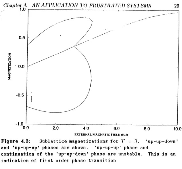
Figure 4.3: S u b la ttic e m agnetizations for T = 3. ’up-up-down’ and ’up-up-up’ phases are shown. ’up-up-up’ phase and

co n tin u a tio n of the ’up-up-down’ phase are u n sta b le. This i s an in d ic a tio n of f i r s t order phase t r a n s itio n

' t r i c r i t i c a li t y ’ b e h a v io u r r»ear th e p h a se tr a n s itio n p o in t frotn d iso rd er e d s t a t e to o r d e r e d s t a t e w ith o u t a m a g n e tic field .

For a d e t a ile d p ic tu r e o f th e p h a se d ia g r a m , it is a lso n e c e ssa r y to e x a m in e u n s t a b le p h a s e s . F ig . '1.1 sh o w s o (d y th e s ta b le p h a se s an d th e t y p e s o f t r a n s it io n s b e tw e e n th e se p h a se s.

E x t e r n a l m a g n e tic field in th e -f- or —

z

d i r e d io u r e su lts in tw o s y m m e t r ic p h a s e s o f m a g n e tiz a tio n . P h a s e d ia g r a m is s y m m e tr ic w ith r e sp e c t to t h e e x t e r n a l m a g n e t ic field d ir e c tio n . T h u s o n ly a p o s itiv e e x te r n a l m a g n e tic field is c h o s e n for la te r d e s c r ip tio n s .

For h ig h e r m a g n e tic field v a lu e s, m a g n e tiz a tio n o f th e s u b la t t ic e s are in t h e s a m e d ir e c tio n as th e e x te r n a l m a g n e tic field . T h e ir m a g n itu d e s are th e s a m e a n d d e p e n d on h ow s tr o n g th e e x te r n a l m a g n e tic field a c tin g on th e s y s t e m is. T h e in te r a c tio n o f th e sp in w ith th e e x te r n a l field d o m in a te s th e

Chapter 4. AN APPlACATiON TO FRUSTRATED SYSTEMS ₃₀

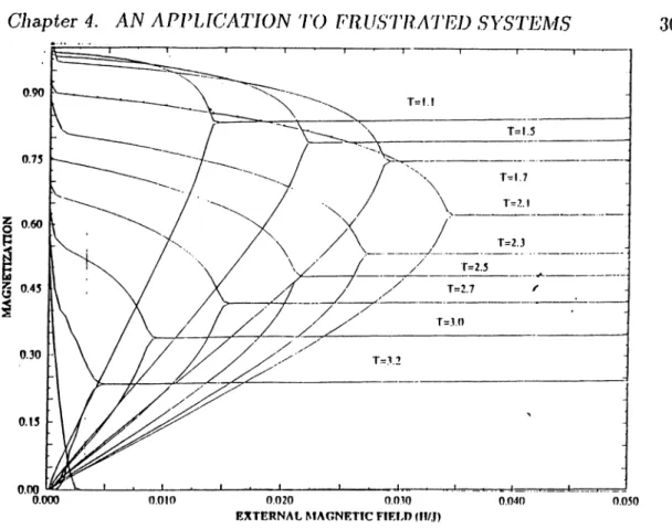
Figure 4.4: S u b l a t t i c e m a g n e t i z a t i o n s f o r d i f f e r e n t t e m p e r a t u r e s . T r a n s i t i o n f r o m ’u p - u p - d o w n ’ p h a s e t o ’u p - z e r o - d o w n ’ p h a s e is s h o w n . T h i s is a n i n d i c a t i o n of s e c o n d o r d e r p h a s e t r a n s i t i o n

phase diagram in this region. When the eiTect of the externa.1 magnetic field is sufficiently small, the contributions from other interaction terms start to appear.

There is a phase transition from the ‘up-up-up’ phase to ‘up-up-down’ phase if the scaled value of the external magnetic field is approximately 6 or lower. This is a first order phase transition in the temperature interval 0 < T < 3 .4 (as in Fig. 4.3) and a second order transition if 3.4 < T < 3.475 (as in Fig. 4.4). For temperatures greater than T > 3.475 there is no phase transition for any value of magnetic field.

First order phase transition can be described in various ways. Calculating the free energy and observing the jump of its value for different phases is one way. The other one is approaching the phase transition point by first decreasing and later increasing the magnetic field and observing the hysterisis effect which is an implication of the first order phase transition. The first one is shown with

Chapter 4. AN APPLICATION TO FRUSTRATED SYSTEMS ₃₁

the closed form solution of hard spin mean field equations. In Fig. 4.3, two different magnetization phases are shown explicitly for T = 3. Here, sublattice magnetizations for different phases are seen to form independent continuous curves. Free energy calculation shows that the up-up-down phase starts to be stable after h j J = 4.5 which is a first order phase trcinsition point.

The phase boundary for this first order phase transition has been calculated by making the same calculation as in Fig. 4.3 to find magnetization for each different temperatures.

If we continue to decrease the external magnetic field, we observe the magnitude of the magnetization changes as is described in Fig. 4.4 for different temperatures. Near the zero external magnetic field we observe a different phase boundary between the ‘up-up-down’ phase and the ‘up-zero-down’. The locus of the critical points for different temperatures form a second order phase transition boundary. This phase boundary increases from zero temperature to T = 2.1 and decreases after that. The implication of a second order phase transition related to this curve is a result of the continuous bifurcation of the magnetizations near the critical points.(see Fig. 4.4.) It is not possible to find the unstable continuation of the phases as in the first order phase transition case. Free energy is also continuous at this point.

The point {T = 3.475, /i = 0) in the phase diagram is a multicritical point. This does not exist in two dimensions. As was described earlier, tricritical or bicritical points occur when there is a third degree of freedom in the system. Here ferromagnetic coupling between the layers corresponds to a third degree of freedom. Therefore, instead of a second order transition point, there is line of second order phase transition in this system. From the phase diagram obtained in the present work it is evident that this is a tricritical point. This is first time observed in this work. In the work of Heinonen^® a tricritical behavior were examined by Monte Carlo simulation but there was no direct evidence for it. In Ref.^^ there is not enough accuracy to state the tricriticality behavior.

The phase diagram can also be understood by considering the external

magnetic field as a parameter. For zero external magnetic field the

Chapter 4. AN APPLICATION TO FRUSTRATFT) SYSTEMS 32

’up-zero-down’) are found easily by taking different initial condition for these two different phases in the hard spin mean field equation. The ‘up-zero-down’ phase is found stable in all temperature based on a free energy calculations. This is different than the previous work whicli suggest a transition point at

t = ,2.1." iFor different values af tlui external magnetic field, the same critical

points as the above were found.

4.2.1

Free E n erg y C a lcu lation s

Among the different phases in the phase diagram, only part of them are stable, the remaining phases may be unstable or metastable. Thermodynamical stability can be understood by the help of free energy calculations.

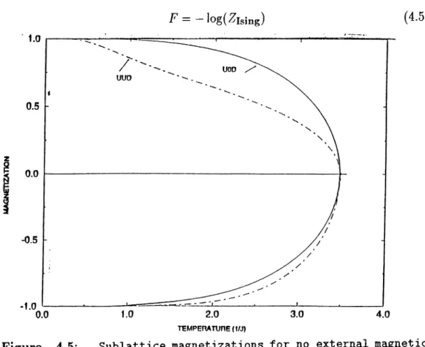
Free energy is calculated as in the Ref.^® Free energy function is defined as

F = — log(Zising) (‘^•^)

TEMPERATUnE (l/J)

Figure 4.5: S u b la ttic e m agnetizations fo r no extern al magnetic f i e l d

Chapter 4. AN APPLICATION TO FlUJSTRATFA) SYSTEMS 33

F i g u r e 4.6: F r e e e n e r g y of t w o p h a s e s in t h e z e r o e x t e r n a l m a g n e t i c f i e l d . ' u p - z e r o - d o w n ’ p h a s e is e n e r g e t i c a l l y f a v o r a b l e at a l l t e m p e r a t u r e s .

which is not same witli the conventional definition of free energy but it is related to it. The calculation of this function is done with a simple trick. First the hard spin average of the derivative of the free energj'^ with respect to coupling constant is calculated, later this quantity is integrated with respect to temperature.

df)F = (l/2A0E.-,-fc(< > + < SkSi >) (4.6) At high temperature with zero magnetic field, free energy of both ‘up-up- down’ phase and ‘up-zero-down’ phase have same value. After transition point (tricritical point) they began to difTerentiate and ‘up,zero-down’ phase become stable. ( That means it has lower free energy.) Resultant free energy for two different phases are shown in Fig. 4;6. This is simply analogous to the relation

C · 6T = dpF ■ ST where C is the specific heat.

For variable magnetic field, free energy can be given as the result of the relation F = M ■ Sh. M is the total sublattice magnetization. Free energy of

‘up-up-up’ phase and ’up-up-down’ phase is drawn in Fig. 4.7. This was used to determine the nature of phase transition (first order phase transition) in the previous section. (This is the reson of jump of the solution from ‘up-up-down’ to ‘up-up-up’ in Fig. 4.7.)

Chapter 4. AN APPLICATION TO FRUSTRATED SYSTEMS 34 2 0 .0 ---IB.O to.o B.O 0.0 0.0 4.0 B.O nrTEnNAI.MAOrtCTir HT.! 0 Figure 4.7: F r e e e n e r g y of t w o p h a s e s f o r

T = 3.

' u p - u p - d o w n ' p h a s e is e n e r g e t i c a l l y f a v o r a b l e at t h e p h a s e t r a n s i t i o n p o i n t t o ' u p - u p - u p ’ p h a s e s .

It is important to start from the same free energy of the two phases (i.e. a reference point) in the calculations. Only the differences of the free energy is im portant to understand the stable phases.

Chapter 5

CONCLUSION

Closed form solutions of the hard spin mean field equations are obtained and applied to the three dimensional stacked triangular lattice system. Phase diagram of this system is analyzed.

The second order phase transition between ‘up-zero-down’ and ‘up-up- down’ phases forms a phase boundary which is not found before. The new phase boundary corresponds to a maximum of magnetic field near T = 2.0 and decreases above and below of this temperature.

The unstable phases were also determined, important to see the first order phase transition characteristic. Free energy calculations were carried out for all phases to analyze thermodynamic stability.

For zero magnetic field system, the ‘up-zero-down’ phase is found to be stable at all temperatures, based on free energy calculations. In contrast, the ‘up-up-down’ phase was found to be stable at lower temperatures in earlier work. This is probably due to the different procedure for the calculations of the magnetizations. In our work a block of three spins were taken for the calculation of the magnetizations in contrast to a single spin in earlier work.

Multicriticality occurs as a result of the meeting of symmetrically different solutions of the order parameter in the same region of the phase diagram.

C hapters. CONCLUSION 36

Critical exponents near the phase transition points depend on the symmetry of the systems. Another new result of our work is the observation of the multicritical region in this system; a tricritical point is found instead of a bicritical point. (This was a debate in previous works.[9],[25])

Hard spin mean field theory has proven to be an adequate method for the frustrated system in three dimensions as well as in two dimensions. It can find further applications as a tool in the examination of different kinds of systems especially different frustrated systems. The closed form solution can also be valuable in the analysis of these systems. For example, Monte Carlo implementation of hard spin mean field theory has been applied to the cubic antiferromagnet. The closed form solution of the equations may be expected to lead to an improvement of the phase diagram of this system.