MEMORY-EFFICIENT MULTILEVEL PHYSICAL
OPTICS ALGORITHM FOR THE SOLUTION OF
ELECTROMAGNETIC SCATTERING PROBLEMS
a thesis
submitted to the department of electrical and
electronics engineering
and the institute of engineering and sciences
of bilkent university
in partial fulfillment of the requirements
for the degree of
master of science
By
Kaplan Alp Manyas
September 2007
I certify that I have read this thesis and that in my opinion it is fully adequate, in scope and in quality, as a thesis for the degree of Master of Science.
Prof. Dr. Levent G¨urel(Supervisor)
I certify that I have read this thesis and that in my opinion it is fully adequate, in scope and in quality, as a thesis for the degree of Master of Science.
Prof. Dr. Adnan K¨oksal
I certify that I have read this thesis and that in my opinion it is fully adequate, in scope and in quality, as a thesis for the degree of Master of Science.
Assist. Prof. Dr. Vakur B. Ert¨urk
Approved for the Institute of Engineering and Sciences:
Prof. Dr. Mehmet Baray
ABSTRACT
MEMORY-EFFICIENT MULTILEVEL PHYSICAL
OPTICS ALGORITHM FOR THE SOLUTION OF
ELECTROMAGNETIC SCATTERING PROBLEMS
Kaplan Alp Manyas
M.S. in Electrical and Electronics Engineering
Supervisor: Prof. Dr. Levent G¨urel
September 2007
For the computation of electromagnetic scattering from electrically large targets, physical optics (PO) technique can provide approximate but very fast solutions. Moreover, higher order approximations, such as physical theory of diffraction (PTD) including the diffraction from the edges or sharp corners can also be added to the PO solution in order to enhance the accuracy of the PO. On the other hand, in real-life radar applications, where the computation of the scatter-ing pattern over a range of frequencies and/or angles with sufficient number of samples is desired, further acceleration may be needed. Multilevel physical op-tics (MLPO) algorithm can be used for such applications, in which a remarkable speed-up can be achieved by evaluating the PO integral in a multilevel fashion. As the correction terms like PTD are evaluated independently just on the edges or sharp corners, whereas the PO integration is carried out on the entire tar-get surface, PO integration is the dominant factor in the computational time of such higher order approximations. Therefore accelerating the PO integration will also reduce the computational time of such higher order approximations. In this thesis, we propose two different improvements on the MLPO algorithm.
First improvement is the modification of the algorithm that enables the solution of the scattering problems involving nonuniform triangulations, thus decreasing the CPU time. Second improvement is the memory-efficient version, in which the
O (N3) memory requirement is decreased to O (N2log N). Efficiency of the two
proposed improvements are demonstrated in numerical examples including a real-life scattering problem, with which the scattering pattern of a three-dimensional stealth target is evaluated as a function of elevation angle, azimuth angle, and frequency.
Keywords: Physical optics; scattering problems; multilevel physical optics
¨
OZET
SAC
¸ ILIM PROBLEMLER˙IN˙IN C
¸ ¨
OZ ¨
UM ¨
U ˙IC
¸ ˙IN BELLE ˘
G˙IN
VER˙IML˙I KULLANILDI ˘
GI C
¸ OK SEV˙IYEL˙I F˙IZ˙IKSEL OPT˙IK
ALGOR˙ITMASI
Kaplan Alp Manyas
Elektrik ve Elektronik M¨uhendisli¯gi B¨ol¨um¨u Y¨uksek Lisans
Tez Y¨oneticisi: Prof. Dr. Levent G¨urel
Eyl¨ul 2007
Fiziksel optik tekni˘gi (FO), elektriksel olarak b¨uy¨uk hedeflerden elektro-manyetik sa¸cılımın hesaplanmasında olduk¸ca hızlı ¸c¨oz¨umler sunabilmektedir. Dahası, gometrinin kenarlarından ve sivri k¨o¸selerinden kaynaklanan kırınım et-kisini de kapsayan kırınımın fiziksel teorisi (KFT) gibi daha y¨uksek dereceli
yakla¸sıklamalarda kullanılarak FO tekni˘ginin hassasiyeti arttırılabilir. ¨Ote
yan-dan, sa¸cılımın belli bir frekans ve/veya a¸cı aralı˘gında, yeterli sıklıkta ¨orneklenerek hesaplanmasının istendi˘gi durumlarda, daha fazla hızlanmaya gereksinim duyu-labilmektedir. Bu ¸ce¸sit uygulamalarda, FO integralinin ¸cok seviyeli bir yakla¸sım
ile hesaplandı˘gı ¸cok seviyeli fiziksel optik algoritması (C¸ SFO) ile b¨uy¨uk ¨ol¸c¨ude
hızlanma sa˘glanabilir. KFT gibi y¨uksek dereceli yakla¸sıklamalarda, kırınım et-kisi, sadece geometrinin kenarlarında ve sivri k¨o¸selerinde hesaplanarak FO
sonu-cuna eklenir. ¨Ote yandan, FO integrali geometrinin t¨um y¨uzeyi ¨uzerinde
he-saplanır ve bu nedenle bu t¨ur yakla¸sıklamaların hesaplanma zamanında belir-leyici unsurdur ve FO integralinin daha hızlı alınması bu t¨ur yakla¸sıklamalarda
da kayda de˘ger bir hızlanma sa˘glayacaktır. Bu tez ¸calı¸smasında, bu
d¨uzensiz ¨u¸cgenlemeleri i¸ceren sa¸cılım problemlerinin de ¸c¨oz¨ulebilece˘gi ¸sekilde de˘gi¸stirilerek, CPU zamanının d¨u¸s¨ur¨ulmesidir. ˙Ikinci iyile¸stirme ise algoritmanın
O (N3) bellek gereksiniminin O (N2log N)’e d¨u¸s¨ur¨uld¨u˘g¨u, belle˘gin verimli
kul-lanıldı˘gı uyarlamasıdır. Sunulan bu iki iyile¸stirmenin verimlilikleri ise, ¨u¸c boyutlu bir hayalet u¸ca˘gın sa¸cılım ¨org¨us¨un¨un y¨ukseli¸s a¸cısına, yanca a¸cısına ve frekansa ba˘glı olarak hesaplandı˘gı, ger¸cek hayatta kar¸sıla¸sılan bir problemin de aralarında bulundu˘gu sayısal ¨ornekler ile sunulmu¸stur.
Anahtar Kelimeler: Fiziksel optik, sa¸cılım problemleri, ¸cok seviyeli fiziksel optik
ACKNOWLEDGMENTS
I would like to thank my supervisor Dr. Levent G¨urel for his supervision, guid-ance, and suggestions throughout the development of this thesis. I would also like to thank him for his support and trust. Without him, I would never had a chance to even start working towards a degree of master of science.
I also thank Prof. Dr. Adnan K¨oksal and Assist. Prof. Vakur B. Ert¨urk for reading and commenting on this thesis.
Contents
1 INTRODUCTION 1 1.1 Historical Background . . . 1 1.2 Motivation . . . 2 1.3 Our Contributions . . . 3 1.4 Outline . . . 3 2 PO APPROXIMATION 4 2.1 Properties of the PO Approximation . . . 82.1.1 Superposition . . . 8 2.1.2 Shift of Origin . . . 9 2.1.3 Frequency Sampling . . . 10 2.1.4 Angular Sampling . . . 13 3 MLPO ALGORITHM 17 3.1 Computation Time . . . 19
3.2 Memory Requirement . . . 19
4 MLPO ALGORITHM FOR NONUNIFORM
TRIANGULA-TIONS 21
4.1 Nonuniform Triangulation . . . 21 4.2 Modified MLPO Algorithm . . . 22 4.3 Results . . . 24
5 MEMORY-EFFICIENT MLPO ALGORITHM 27
5.1 Results . . . 30
5.1.1 Bistatic RCS of the Flamme Geometry . . . 30
5.1.2 Backscattering RCS of the Flamme Geometry . . . 35
6 CONCLUSIONS 41
APPENDIX 43
A Lagrange Interpolation 43
A.1 One-Dimensional (1-D) Lagrange Interpolation . . . 43 A.2 Three-Dimensional (3-D) Lagrange Interpolation . . . 44 A.3 Lagrange Interpolation Near the End Points . . . 46
B Accuracy of the PO Approximation 50
List of Figures
2.1 PO surface current density: (a) For horizontally polarized electric
field incidence. (b) For vertically polarized electric field incidence. 5
2.2 Uniform meshes of arbitrary targets: (a) Sphere, (b) cube,
(c) a stealth target, and (d) a plane. . . 6
2.3 Nonuniform meshes of arbitrary targets: (a) Cube with smooth
edges, (b) a stealth target, and (c) another stealth target. . . 7
2.4 Triangle for the analytic evaluation of the PO integral. . . 8
2.5 Shift of the surface S by a vector r0. . . 9
2.6 Illustration of the smallest sphere that can contain the target. . . 10 2.7 A helicopter model and the illustration of the smallest sphere that
can contain it. . . 11
2.8 Spectrum of the Escat signal as a function of frequency for the
backscattering case. The resolved bands for different oversampling ratios are also shown in the same figure. . . 11 2.9 Increase of accuracy as the sampling rate increases. . . 12
2.10 Spectrum of the Escat signal as a function of φ for the
backscat-tering case. The resolved bands for different oversampling ratios are also shown in the same figure. . . 15 2.11 Increase of accuracy as the sampling rate increases. . . 16
3.1 Calculating the scattering pattern of S as a sum of scattering
patterns of smaller subsurfaces S1 and S2. . . 18
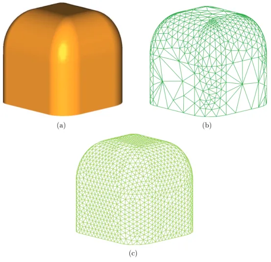
4.1 An example geometry with both smooth and curved regions: (a) Shaded view. (b) A uniform triangulation example. (c) A nonuniform triangulation example. . . 22 4.2 Aggregation of larger triangles. (a) Aggregating at the bottom
level with a lower sampling rate, which will cause an interpolation error. (b) Aggregating at higher levels with the correct sampling rate, which will prevent the interpolation error. . . 23 4.3 Generic helicopter geometry . . . 24 4.4 Backscattering RCS pattern of the generic helicopter
geome-try, computed via direct PO integration and MLPO algorithm: (a) RCS results. (b) Normalized error between the complex scat-tered fields. . . 25 4.5 Backscattering RCS pattern of the generic helicopter geometry,
computed via MLPO algorithm for uniform and nonuniform tri-angulations. . . 26
5.1 Aggregation steps in the proposed memory-efficient algorithm. Note that θ ∈ [0 : ∆θ : 180] means that the patterns at that level is sampled from 0 to 180, with an increment of ∆θ . . . 28
5.2 Aggregations of pattern portions for a 6-level problem. Aggrega-tions are shown as blue arrows and output to files are shown as red arrows. . . 29 5.3 Interpolating cluster patterns near the end points. . . 30 5.4 Geometry of the stealth Flamme target: (a) Front view. (b) A
uniform mesh example. (c) Rear view. (d) Top view. . . 31 5.5 Bistatic RCS pattern of the Flamme geometry computed with
direct PO evaluation: (a) x-y, (b) x-z, and (c) z-y planes. . . 32 5.6 Bistatic RCS pattern of the Flamme geometry computed with
MLPO algorithm: (a) x-y, (b) x-z, and (c) z-y planes. . . 33 5.7 Absolute error of the MLPO algorithm: (a) x-y, (b) x-z, and
(c) z-y planes. . . 34 5.8 Efficiency of the MLPO algorithm: (a) CPU time. (b) Memory
requirement. Dashed curves represent estimated values. . . 35 5.9 Backscattering RCS pattern of the Flamme geometry computed
with direct PO evaluation: (a) x-y, (b) x-z, and (c) z-y planes. . . 36 5.10 Backscattering RCS pattern of the Flamme geometry computed
with MLPO algorithm: (a) x-y, (b) x-z, and (c) z-y planes. . . 37 5.11 Absolute error of the MLPO algorithm: (a) x-y, (b) x-z, and
(c) z-y planes. . . 38 5.12 Efficiency of the MLPO algorithm: (a) CPU time. (b) Memory
A.1 Implementation of 2-D Lagrange interpolation with 1-D Lagrange
interpolations. Since V0 and V1 are calculated previously,
cal-culating V2 requires summation of only two terms, whereas 2-D
interpolation would require summation of four terms. . . 45 A.2 Using the derivative information at the points that are close to
the interpolated sample near the end points. . . 47
B.1 PO and analytical solutions for the backscattering RCS of a sphere with radius a. . . 51 B.2 Rectangular prism. . . 52 B.3 Bistatic scattering from the rectangular prism on the z-y plane. . 52 B.4 Bistatic scattering from the rectangular prism on the x-z plane. . 53 B.5 Helicopter model. . . 53 B.6 Bistatic scattering from the helicopter model on the x-z plane. . . 54
List of Tables
4.1 Computation of the generic helicopter model’s RCS pattern: Num-ber of triangles and CPU times for direct PO evaluation, MLPO algorithm, and modified MLPO algorithm with nonuniform trian-gulation. . . 24
5.1 Computation of the Flamme’s bistatic RCS pattern: Growth of the number of triangles, θ samples, φ samples, and frequency sam-ples as N increases . . . 31
Chapter 1
INTRODUCTION
Physical optics (PO) is a high-frequency technique that can offer quick but ap-proximate solutions for the scattering problems involving smooth, convex, and electrically large targets. On the other hand, speed-up for even PO can be needed for problems, for which the solutions are desired in a range of frequencies and/or angles.
1.1
Historical Background
Current-based high-frequency techniques, such as PO [1] and physical theory of diffraction (PTD) [2], are widely used asymptotic techniques to approximate the solution of the electromagnetic scattering from electrically large, convex, and smooth targets. In those techniques, PO integration is the dominant factor in the computational time since the additional correction terms are usually in the form of line integrals along the edges or wedges. For scattering problems with complex targets, MLPO algorithm turns out to be a suitable approach to decrease the PO integration time [6].
1.2
Motivation
To find the PO scattering pattern of a target, the integral
Es(r) = −jkηe−jkr 2πr Z S ˆ n (r0) × Hi 0ejk(ˆr−ˆri)·r 0 ds0 (1.1)
should be evaluated on the lit regions of the target. In this equation, r0 is the
source point on S, ˆn (r0) is the normal of the surface at r0, Hi
0 is the incident
magnetic field vector, ˆr is the unit vector along the direction of observation, and
ˆri is the unit vector along the direction of incidence. As the target surface can
be arbitrarily complex, obtaining an explicit solution for this integral is usually impossible. Therefore, dividing the surface area into triangles and evaluating the PO integral analytically on each triangle is a common approach [8]. PO integral evaluated in this manner takes the form of
Es(r) = −jkη−e jkr 2πr T X k=1 ˆ nk× Hi0 Z ∆k ejk(ˆr−ˆri)·r0ds0, (1.2)
where T is the total number of triangles. Let R be the radius of the smallest sphere that can contain the target and N = kR, where k is the wavenumber.
Then, the total number of triangles will be proportional to N2.
In order to be able to interpolate such a scattering pattern from its samples with a prescribed error, the sampling rate should be proportional to the electrical size of the target. The required number of samples in θ, φ, and frequency are O (N) each.
Therefore, computational complexity of finding the scattering pattern over a range of frequencies and angles with sufficient number of samples turns out to be
be reduced to O (N3log N) without sacrificing the accuracy, but with a memory
cost of O (N3log N).
1.3
Our Contributions
In this thesis, two-dimensional (2-D) MLPO algorithm proposed by Boag [6] is applied to 3-D problems. We also propose two improvements on the MLPO algorithm. First improvement is the modification of the algorithm that enables the solution of the scattering problems involving nonuniform triangulations, thus decreasing the CPU time. Second improvement is the memory-efficient version,
in which the O (N3) memory requirement is decreased to O (N2log N).
1.4
Outline
In Chapter 2, we first introduce the PO approximation. In Chapter 2, we also mention the properties of the PO approximation that are basic tools for the MLPO algorithm presented in Chapter 3. The MLPO algorithm for nonuniform triangulations is proposed in Chapter 4, where the computational efficiency of the proposed algorithm is also demonstrated. We propose the memory-efficient MLPO algorithm in Chapter 5 and demonstrate its memory efficiency. We con-clude and list future research areas in Chapter 6.
Chapter 2
PO APPROXIMATION
Integral-equation methods, such as the method of moments [3], fast multipole method [4], and multilevel fast multipole method [5], in which the current is solved to satisfy the boundary condition, are usually impractical for electrically large problems. This is because, in these methods, the required computational resources increase rapidly with the electrical size of the problem. On the other
hand, in the PO approximation, the surface current Js is assumed to be
Js = 2ˆn × Hinc (2.1)
in the lit regions, instead of being solved. This assumption offers less accurate
but faster solutions. Here ˆn is the surface normal and Hinc is the incident
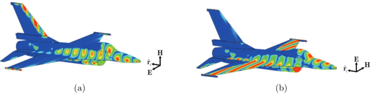
magnetic field. In Fig. 2.1, the induced PO currents on an F-16 plane is given as an illustration for horizontally and vertically polarized incidences. Under
this assumption, for a plane-wave incidence Hinc(r) = Hinc
0 e−jkr·ˆri, the far-field radiation integral Escat(r) = −jkηe −jkr 4πr Z Js(r0)ejkˆr·r 0 dr0 (2.2)
takes the form of
Escat(r) = −jkηe−jkr 2πr Z r0∈Slit b n × Hinc 0 ejkr 0·(ˆr−ˆr i)dr0. (2.3)
ˆi r E H (a) ˆi r H E (b)
Figure 2.1: PO surface current density: (a) For horizontally polarized electric field incidence. (b) For vertically polarized electric field incidence.
In operator notation, ΨS = −jkηe−jkr 2πr Z r0∈Slit b n × Hinc 0 ejkr 0·(ˆr−ˆr i)dr0, (2.4)
where Ψ is the PO operator evaluating the scattering pattern of S. Note that
the r0 dependence of ˆn is suppressed for simplicity. Since it is difficult to evaluate
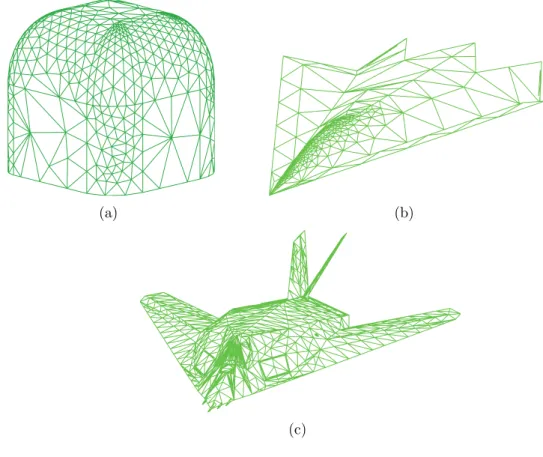
the integral in Equation (2.3) analytically for an arbitrary complex 3-D target, triangulation or triangular meshing is a common approach for modeling 3-D targets with arbitrary complex geometries. Triangulations of various geometries are shown in Figs. 2.2 and 2.3.
In a uniform triangulation, the triangle size (or mesh size) is usually chosen approximately between λ/10 and λ/5 depending on the desired accuracy. In a nonuniform triangulation, the triangle size can be adjusted locally according to the surface curvature. More detailed description of nonuniform triangulation is presented in Section 4.1.
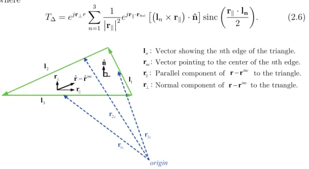
After the triangulation of the geometry, Gordon’s well-known formula for the analytic evaluation of PO integral over planar patches [8] can be used to evaluate the PO radiation from each triangle. For a single triangle ∆ shown in Fig. 2.4, this formula reduces to
Escat∆ (r) = −jk−e jkr 2πr ¡ ˆ n∆× Hinc0 ¢ T∆, (2.5)
(a) (b)
(c) (d)
Figure 2.2: Uniform meshes of arbitrary targets: (a) Sphere, (b) cube,
(a) (b)
(c)
Figure 2.3: Nonuniform meshes of arbitrary targets: (a) Cube with smooth edges, (b) a stealth target, and (c) another stealth target.
where T∆ = ejr⊥r 3 X n=1 1 ¯ ¯rk ¯ ¯2ejrk·rnc £¡ ln× rk ¢ · ˆn¤sinc µ rk· ln 2 ¶ . (2.6) 1 l 3 l 2 l 1c r 2c r 3c r ˆ nˆ n || r ˆ ˆinc − r r ⊥ r : : : : n nc ⊥ l r r r P
Vector showing the nth edge of the triangle. Vector pointing to the center of the nth edge. Parallel component of to the triangle. Normal component of to the trıangle.
inc − r r inc − r r origin
Figure 2.4: Triangle for the analytic evaluation of the PO integral.
Since Equation (2.6) is a closed-form expression with no integrals, it offers accu-rate and efficient evaluation of the PO integral over a single triangle. Afterwards, the radiation pattern from each triangle can be added to find the overall scatter-ing pattern as Escat= Nt X n=1 E∆scatn . (2.7)
2.1
Properties of the PO Approximation
The properties of the PO approximation listed below are the basis of the MLPO algorithm presented in Chapter 3.
2.1.1
Superposition
If the target surface S is split into non-overlapping subsurfaces, then the su-perposition of the radiation patterns of these subsurfaces will be equal to the
scattering pattern of S as ΨS = Q X q=1 ΨSq. (2.8)
In addition to allowing the triangulation of the target surface and evaluation of the PO integral separately on each triangle, this property will be used to group the triangles and their scattering patterns in the MLPO algorithm presented in Chapter 3.
2.1.2
Shift of Origin
Let O [r0] denote an operator shifting the target surface by vector r0as in Fig. 2.5.
Then, direct substitution of r0 = r0− r
0 in Equation (2.4) yields
O [r0] ΨS = ejk(ˆr−ˆri)·r0ΨS. (2.9)
Similarly, E [r0], which is the inverse of O [r0], can be defined as O [−r0], where
O [r0] and E [r0] denote multiplication by e−jkr0·(ˆr−ˆri)and ejkr0·(ˆr−ˆri), respectively.
This property is essential for removing the extra phase oscillations from complex
1
S
Ψ
(ˆ ˆi) 0 jke
r r r− ⋅ x y z x y z x y z 0r
1S
2S
1 scatE
= Ψ
S
2 scatE
= Ψ
S
=
Figure 2.5: Shift of the surface S by a vector r0.
scattering patterns before the interpolation in the MLPO algorithm to be pre-sented in Chapter 3.
2.1.3
Frequency Sampling
When considered as a function of frequency, the PO scattering pattern in Equa-tion (2.4) can be written as
ΨS = −jkηe −jkr 2πr Z r0∈Slit b n × Hinc0 ej2πfc r0·(ˆr−ˆri)dr0. (2.10)
This expression is in fact the superposition of exponential terms ejr0·(ˆr−ˆc ri)2πf. If R
is the radius of the smallest sphere that can contain the target as in Fig. 2.6, then r0·(ˆr−ˆr
i)
c can take a maximum value of 2R/c. This occurs when ˆr−ˆri
(backscatter-ing case) and r0 is in the same direction with ˆr = −ˆr
i. According to the Nyquist
S
R N=kR
Figure 2.6: Illustration of the smallest sphere that can contain the target. sampling theorem [10], f should be sampled with ∆f < c/4R, where ∆f is the sampling period of f . As a consequence, in order to allow interpolation, the required number of frequency samples is
Nf = Ωf
4R (fmax− fmin)
c , (2.11)
where Ωsis a real number greater than 1 indicating the ratio of the sampling rate
to the theoretical one. As a result, the number of frequency samples is O (N), where N = kR.
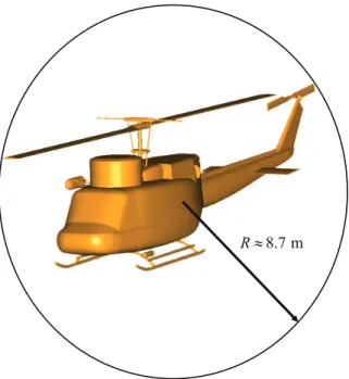
In Fig. 2.8, spectrum of the backscattering signal from a helicopter model shown in Fig. 2.7 is presented in order to verify the validity of Equation (2.11). In the same figure, the resolved band for different oversampling ratios are also shown.
8.7 m
R ≈
Figure 2.7: A helicopter model and the illustration of the smallest sphere that can contain it.
−600 −400 −200 0 200 400 600 10−4 10−3 10−2 10−1 100 time (nanoseconds) F { E scat (f) }
Normalized spectrum of the Fourier transform of Escat.
Escat is sampled as a function of frequency in the [0, 20] GHz range.
Spectrum Of The Frequency Sweep Resolved Spectrum For Ωf = 10.1588 Resolved Spectrum For Ωf = 3.5871 Resolved Spectrum For Ωf = 2.1781 Resolved Spectrum For Ωf = 1.5638 Resolved Spectrum For Ωf = 1.2198
Figure 2.8: Spectrum of the Escat signal as a function of frequency for the
backscattering case. The resolved bands for different oversampling ratios are also shown in the same figure.
From Fig. 2.8, it is observed that Ωf ≈ 1 is sufficient to resolve the harmonics
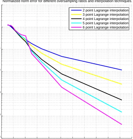
having a normalized weight of 10−4. On the other hand, in Fig 2.9, it is shown
that in order to have a norm error
kerrorknormalized = °
°Sref − Sip°°
kSipk (2.12)
below 10−3, the oversampling ratio in frequency should be greater than 3. Note
that Sref is the reference signal and Sip is the interpolated signal in
Equa-tion (2.12). 0 0.5 1 1.5 2 2.5 3 3.5 4 4.5 5 5.5 10−5 10−4 10−3 10−2 10−1 100 101 Ωf (oversampling Ratio)
Normalized norm error ||S
ref
− S
ip || / ||S
ref
||
Normalized norm error for different oversampling ratios and interpolation techniques. 2 point Lagrange interpolation 3 point Lagrange interpolation 4 point Lagrange interpolation 5 point Lagrange interpolation 6 point Lagrange interpolation
Figure 2.9: Increase of accuracy as the sampling rate increases. .
Fig 2.9 also shows that by employing different number of points in the interpo-lation, the interpolation error can be decreased for a given oversampling ratio.
It should be noted since the Lagrange interpolation is a local interpolation, in-creasing the number of points does not increase the computational complexity for uniformly sampled data. More detailed discussion of the Lagrange interpolation can be found in Appendix.
2.1.4
Angular Sampling
As mentioned in Section 2.1.3, the PO scattering pattern has the largest
oscilla-tion rate for the backscattering case, where ˆri = −ˆr. For the sake of simplicity,
the minimum angular sampling rate will be derived for the backscattering case, which is also applicable to the bistatic case. For the backscattering case, the PO scattering pattern in Equation (2.4) can be written as
Escat(r) = −jkηe−jkr 2πr Z r0∈Slit b n × Hinc 0 e2jkr
0[sin(θ) sin(θ0) cos(φ−φ0)+cos(θ) cos(θ0)]
dr0.
(2.13)
In this expression, (θ, φ) and (θ0, φ0) are the elevation and azimuth angles of the
direction of scattering and the direction of source point, respectively. For the backscattering case, as a function of φ, PO scattering pattern in Equation (2.4) can be written as Escat(r) = −jkηe−jkr 2πr Z r0∈Slit b n × Hinc 0 ej4πf r 0cos(θ) cos(θ0)
ej4πf r0sin(θ) sin(θ0) cos(φ−φ0)
dr0.
(2.14) This expression can be thought of as the superposition of exponential terms of
type ejβ cos(φ−φ0)
, where β = 4πf r0sin (θ) sin (θ0). Fourier series expansion of these
terms yields [9] ejβ cos(φ−φ0) = J0(β) + 2 ∞ X n=1 jnJ n(β) cos [n (φ − φ0)]. (2.15)
Here Jn(·) represents the Bessel function of order n. Since Bessel functions decay
β. As the maximum value that β can take is 4πf R/c, the maximum oscillation
rate of the harmonics in Equation (2.15) is bounded with 4πf R/c. From Nyquist sampling theorem, the sampling rate in φ must be twice this value. Therefore,
∆φ, which is the sampling interval in φ, should be at most c/8πfmaxR. As a
consequence, for an angular range of [0, 2π], the number of φ samples is
Nφ= Ωφ
8πfmaxR
c . (2.16)
Therefore, the number of φ samples that will allow interpolation grows with
O (N). Similarly, the number of θ samples is Nθ = Ωθ
4πfmaxR
c (2.17)
since θ is to be sampled in the [0, π] range instead of [0, 2π]. Here Ωφand Ωθ are
real numbers greater than 1 indicating the ratio of the actual sampling rates to the theoretical ones.
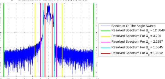
As in the frequency sampling section, in order to verify the validity of Equa-tion (2.11), spectrum of the backscattering from a helicopter model (Fig. 2.7) is given in Fig. 2.8. In the same figure, the resolved band for different oversampling ratios are also shown.
From Fig. 2.8, it is observed that increasing Ωφ beyond 3 does not decrease the
norm error significantly. This can be explained by the illumination effect. By employing the visibility function
V (r0) = 1, r0 ∈ S lit 0, otherwise , (2.18)
PO operator given in Equation (2.4) can be written as
ΨS = −jkηe −jkr 2πr Z r0∈S V (r0) bn × Hinc0 ejkr0·(ˆr−ˆri)dr0. (2.19)
It is clear that since bn × Hinc
0 term in the Fourier transform integral is multiplied
−12 −10 −8 −6 −4 −2 0 2 4 6 8 10 12 10−4 10−3 10−2 10−1 100 1/degree F { E scat ( φ ) }
Normalized spectrum of the Fourier transform of Escat.
Escat is sampled as a function of φ in the [0, 2π] range.
Spectrum Of The Angle Sweep Resolved Spectrum For Ωφ = 12.5649 Resolved Spectrum For Ωφ = 3.796 Resolved Spectrum For Ωφ = 2.2357 Resolved Spectrum For Ωφ = 1.5845 Resolved Spectrum For Ωφ = 1.0012
Figure 2.10: Spectrum of the Escatsignal as a function of φ for the backscattering
case. The resolved bands for different oversampling ratios are also shown in the same figure.
broadened. This fact can be verified from Fig. 2.10, where the spectrum of the scattered signal decays slower compared to Fig. 2.8. In addition, as the PO operator given in Equation (2.19) is evaluated on a coarse grid at the bottom level, illumination is also computed for this coarse grid. Therefore at each level, illumination is also interpolated with scattering patterns of the subdomains.
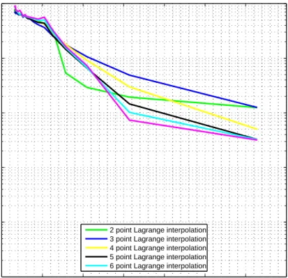
0 1 2 3 4 5 6 7 10−4 10−3 10−2 10−1 100 Ωφ (oversampling ratio)
complex error norm (normalized)
||E re f − E IP || / ||E re f ||
Normalized norm error for different oversampling ratios and interpolation techniques.
2 point Lagrange interpolation 3 point Lagrange interpolation 4 point Lagrange interpolation 5 point Lagrange interpolation 6 point Lagrange interpolation
Chapter 3
MLPO ALGORITHM
When computing the PO scattering pattern with sufficient number of samples as a function of θ, φ, and frequency, sampling rate in each dimension should be proportional to the electrical size of the target. Let R be the smallest radius of a sphere that can contain the target and N = kR, where k is the wavenumber. Then, the required number of samples in θ, φ, and frequency are O (N) each and
the total number of required samples is O (N3) . If the target surface is modeled
with a triangular mesh, there will be O (N2) triangles as the number of triangles
will be proportional to the surface area. Hence, the computational complexity of evaluating the PO integral analytically [8] on the triangular mesh for each
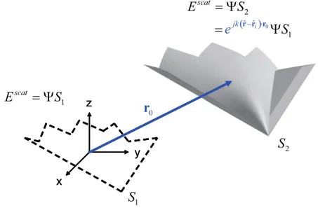
θ, φ, and frequency turns out to be O (N5). The MLPO algorithm aimed to decrease this complexity is based on the decomposition of the target surface S into nonoverlapping subdomains. Since each subdomain will have a smaller size, its scattering pattern can be sampled at a rate lower than the rate required for the scattering pattern of S as a whole. After the evaluation of the subdomain scattering patterns at lower sampling rates, these patterns can be aggregated to find the scattering pattern of the whole geometry. As the pattern evaluated by the aggregation of the smaller subdomain patterns will be larger, the subdomain
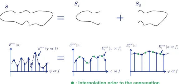
scattering patterns should be interpolated to a finer grid before aggregation. This scheme is illustrated in Fig. 3.1.
[ ] 1 scat E n or f ϕ ( ) 1 or scat E ϕ f
: Interpolation prior to the aggregation [ ] scat E n or f ϕ ( or ) scat E ϕ f 2 [ ] scat E n or f ϕ ( ) 2 or scat E ϕ f
= +
= +
S1 S2 S=
Figure 3.1: Calculating the scattering pattern of S as a sum of scattering patterns
of smaller subsurfaces S1 and S2.
Since the origin of each subdomain will be different from the global origin, subdo-main patterns will oscillate at higher rates because of the phase shift (Fig. 2.5). Therefore, prior to interpolation, subdomain patterns should be shifted to the origin and restored after interpolation. In this scheme, PO operator Ψ that computes the scattering pattern of any arbitrary surface S can be written as
ΨS =XQ
q=1E [¯rq] I NθNφNf
¯
NθN¯φN¯fO [¯rq] Ψ ¯Sq. (3.1)
Here, ¯rq is the center of the smallest sphere that can include the qth subdomain.
O [¯rq] is the operator that shifts the origin of the qth subdomain to the global
origin in order to remove the phase oscillations. The INθNφNf
¯
NθN¯φN¯f matrix is the
inter-polation matrix that increases the number of samples from ¯Nθ× ¯Nφ× ¯Nf points
to Nθ× Nφ× Nf points, and E [¯rq] is the operator that shifts the origin of the qth
subdomain back to its location after the interpolation. Efficient implementation
of interpolation INθNφNf
¯
NθN¯φN¯f is given in Appendix A.
In the MLPO algorithm, each subdomain Sqis recursively subdivided into smaller
subdomains and the scattering patterns of these subdomains are also calculated using the PO operator Ψ in Equation (3.1). When the subdomain size is in the
order of λ (wavelength), the subdivision process is stopped and the scattering patterns of the lowest-level subdomains are evaluated with the direct evalua-tion of the PO integral. Hence in the MLPO algorithm, the PO operator Ψ in Equation (3.1) takes the form of
ΨS =XQ q=1E [¯rq] I NθNφNf ¯ NθN¯φN¯fO [¯rq] XQ q=1E [¯rq] I NθNφNf ¯ NθN¯φN¯fO [¯rq] · · · Ψ ¯Sq. (3.2)
3.1
Computation Time
As the electrical size of the bottom-level subdomains will be bounded, the re-quired number of θ, φ, and frequency samples will be fixed for each subdomain at
this level. There will be O (N2) filled subdomains at this level and therefore
cal-culating the PO patterns of all subdomains analytically at this level will require
O (N2) operations. At each aggregation step, local interpolations transforming
the scattering patterns form a coarse grid of θ, φ, and frequency to a finer grid will
require O (N3) operations. As there will be O (log N) levels, total computational
cost of aggregations will be O (N3log N). Therefore, the overall computational
complexity of the MLPO algorithm is O (N2) + O (N3log N) = O (N3log N).
This complexity is far less than the O (N5) complexity of the conventional PO
integration.
3.2
Memory Requirement
As mentioned before, the number of pattern samples in the bottom level is fixed and does not grow with N. Since the number of subdomains in the bottom level
is O (N2), memory required to store the scattering patterns of the bottom-level
subdomains is also O (N2). When aggregating from lower levels to the upper
only on the surface of the target, we can assume that the number of filled clusters is reduced by a factor of 4 at each higher level. Therefore, memory required at each aggregation step will increase by a factor of 8/4 = 2. Hence, at the
uppermost level, memory requirement will be O¡N22log N¢, which is O (N3). As
will be shown in Chapter 5 , this memory requirement may prevent the solution of larger problems using the MLPO algorithm. In Chapter 5, we present a
memory-efficient implementation that reduces the memory complexity from O (N3) to
Chapter 4
MLPO ALGORITHM FOR
NONUNIFORM
TRIANGULATIONS
4.1
Nonuniform Triangulation
In electromagnetic scattering problems, triangulation or triangular meshing is a common approach for modelling targets with complex geometries. In a uniform triangulation, the triangle size (or mesh size) is usually chosen approximately between λ/10 and λ/5 depending on the desired accuracy. In this scheme, the number of triangles is directly proportional to the surface area of the target and
the complexity of the number of triangles grows with O (N2).
On the other hand, if a nonuniform triangulation is employed, instead of ad-justing the size of each triangle approximately equal to some fraction of λ, the triangle size can be adjusted according to the surface curvature of the target, i.e., the triangle size gets smaller where the curvature is high and larger where the curvature is low. In such a triangulation, the size of each triangle can be
iteratively modified until the scattering pattern of each subdomain, evaluated via PO, converges [7]. Alternatively, the size of each triangle can be adjusted until the distance of each triangle from the target surface is less than a predefined deviation. Second alternative is chosen for simplicity in the example problems that demonstrate the application of the MLPO algorithm on nonuniform trian-gulations.
(a) (b)
(c)
Figure 4.1: An example geometry with both smooth and curved regions: (a) Shaded view. (b) A uniform triangulation example. (c) A nonuniform trian-gulation example.
4.2
Modified MLPO Algorithm
As mentioned in Chapter 3, in the MLPO algorithm, only the scattering pat-terns of the smallest subdomains are computed via PO and those patpat-terns are
sampled at lower rates according to their dimensions. In a nonuniform trian-gulation, there may be triangles that are too large to fit in the smallest subdo-mains. Since the required sampling rate for the patterns of these triangles will be higher, sampling and aggregation of these triangles in the lowest levels will result in an interpolation error that grows at each aggregation step as illustrated in Fig. 4.2(a). Therefore the MLPO algorithm is modified in such a way that the radiation patterns of the larger triangles are sampled at a rate proportional to their dimensions and aggregated at the appropriate levels as in Fig. 4.2(b).
[ ] 1 s E n f ( ) 1 s E f
. . .
I I I I I I I I I I I I I I. . .
I I I I I I I I I I I I. . .
I I I I I II I I I I I I I I I I I I I I I I II I I I I I I I I I I I I I f ( ) 2 s E f [ ] 2 s E n (a) [ ] 1 s E n f ( ) 1 s E f. . .
I I I I I I I I I I I I I I. . .
I I I I I I I I I I I I. . .
I I I I I II I I I I I I I I I I I I I I I I II I I I I I I I I I I I I I f ( ) 2 s E f [ ] 2 s E n (b)Figure 4.2: Aggregation of larger triangles. (a) Aggregating at the bottom level with a lower sampling rate, which will cause an interpolation error. (b) Aggre-gating at higher levels with the correct sampling rate, which will prevent the interpolation error.
Table 4.1: Computation of the generic helicopter model’s RCS pattern: Number of triangles and CPU times for direct PO evaluation, MLPO algorithm, and modified MLPO algorithm with nonuniform triangulation.
Direct PO MLPO Modified MLPO algorithm
evaluation algorithm with nonuniform triangulation
Number of triangles 88,000 88,000 24,000
CPU time 5.7 min 0.26 min 0.075 min
4.3
Results
To illustrate the efficiency of the improved MLPO algorithm for nonuniform
triangulations, the geometry shown in Fig. 4.3 is illuminated from the (θi, φi) =
(135◦, 90◦) direction. The RCS results computed with PO and MLPO algorithm
are shown in Fig. 4.4
16 m
3.5 m
x y
z
Figure 4.3: Generic helicopter geometry
In Fig. 4.4, RCS results and the error between the RCS patterns calculated with PO integration and MLPO algorithm is presented. It is seen that the error in RCS is below 1%.
The scattering pattern is evaluated for 577 points in the frequency range of [0.1, 1] GHz via direct PO evaluation, MLPO algorithm, and the modified MLPO algorithm for nonuniform triangulations. The number of triangles and CPU times are given in Table 4.1.
0.2 0.4 0.6 0.8 1 5 10 15 20 25 30 Frequency (GHz) RCS (dBms)
Backscattering RCS results of the generic helicopter model. θ: 135° φ: 90°
PO MLPO (a) 0.2 0.4 0.6 0.8 1 −40 −35 −30 −25 −20 −15 −10 −5 0 Frequency (GHz) 10log 10 |RCS M L P O − RCS P O |
Error between backscattering RCS Patterns
(b)
Figure 4.4: Backscattering RCS pattern of the generic helicopter geometry, com-puted via direct PO integration and MLPO algorithm: (a) RCS results. (b) Nor-malized error between the complex scattered fields.
0.2 0.4 0.6 0.8 1 5 10 15 20 25 30 Frequency (GHz) RCS (dBms)
Backscattering RCS results of the generic helicopter model. θ: 135° φ: 90°
MLPO (nonuniform triangulation) MLPO (uniform triangulation)
Figure 4.5: Backscattering RCS pattern of the generic helicopter geometry, com-puted via MLPO algorithm for uniform and nonuniform triangulations.
The nonuniform triangulation consists of approximately 24,000 triangles. The CPU time of the MLPO with uniform triangulation of 6 cm is 0.26 min. On the other hand, CPU time of MLPO with the nonuniform triangulation is 0.075 min. Although a up of nearly 3.5 may seem insufficient, a greater speed-up can be achieved by increasing the deviation of the nonuniform mesh from the geometry and thereby decreasing the accuracy. Moreover, uniform triangulations may require millions of triangles in real-life applications with target sizes up to thousands of λ. Therefore, even generating such triangulations for complex geometries may become impossible and a nonuniform triangulation may become a good choice.
Chapter 5
MEMORY-EFFICIENT MLPO
ALGORITHM
The proposed memory-efficient implementation of the MLPO algorithm is based on the idea that, the patterns of the clusters need not be stored for the entire range of θ, φ, or frequency values at the same time. By a careful implementa-tion, the θ, φ, or frequency ranges can be divided into smaller ranges so that interpolations and aggregations can be performed on those smaller ranges. For instance, when aggregating the bottom level to the upper level, θ can be
sampled in the £0,π
2 ¤
range instead of [0, π]. This way, the memory required for each cluster will grow by a factor of 4 instead of 8. In the next level, the number of clusters will be reduced by a factor of 4, and the total required memory will
be constant. Then, θ can be sampled in the£0,π
4 ¤ range instead of £0,π 2 ¤ at the next level, and this procedure can be applied till the uppermost level is reached. This scheme is illustrated in Fig. 5.1.
If L is the number of levels, after the aggregations are performed, 1±2L−1portion
of whole scattering pattern will be available at the Lth level. This portion can be output to a file and the remaining portion can be obtained by aggregating the
. . . [0 : : ] samples Nθ θ∈ ∆θ π 0 : : 2 2 samples N θ θ π θ∈ ∆ 0 : : 4 4 samples Nθ θ π θ∈ ∆ . . .
Figure 5.1: Aggregation steps in the proposed memory-efficient algorithm. Note that θ ∈ [0 : ∆θ : 180] means that the patterns at that level is sampled from 0 to 180, with an increment of ∆θ
second half to Lth level. Then the 3rd portion of the pattern will be required. This portion will not be available at the (L − 1)st level. Therefore, the pattern available at the (L − 2)nd level should be aggregated to the (L − 1)st level. The 3rd portion of the whole scattering pattern at the Lth level can be obtained
by aggregation from the (L − 1)st level. In this scheme, after 2L−1 passes, the
whole scattering pattern will be obtained. As an example, aggregations of pattern portions for a 6 -level problem is depicted in Fig. 5.2.
The following pseudo-code describes the partial aggregation of the clusters at each pass:
{n is an array of size L − 1, indicating which half of the available pattern
portion should be aggregated at each pass.}
{In the first pass, first halves of the available pattern portions should be
ag-gregated.}
n(1 : L) ← 1
for t = 1 to 2L−1 do
for l = 1 to L − 1 do {all levels 1 to L − 1}
m ← L − l + 1
passes le v e ls
. . .
output to file output to file output to file output to file output to file output to file output to file output to file output to file 1 0, 32 2 0, 32 4 0, 32 8 0, 32 16 0, 32 32 0, 32 2 0, 32 2 0, 32 4 0, 32 8 0, 32 16 0, 32 32 0, 32 2 3 , 32 32 2 4 , 32 32 4 0, 32 8 0, 32 16 0, 32 32 0, 32 3 4 , 32 32 2 4 , 32 32 4 0, 32 8 0, 32 16 0, 32 32 0, 32 4 5 , 32 32 4 6 , 32 32 4 8 , 32 32 8 0, 32 16 0, 32 32 0, 32 5 6 , 32 32 4 6 , 32 32 4 8 , 32 32 8 0, 32 16 0, 32 32 0, 32 6 7 , 32 32 6 8 , 32 32 4 8 , 32 32 8 0, 32 16 0, 32 32 0, 32 7 8 , 32 32 6 8 , 32 32 4 8 , 32 32 8 0, 32 16 0, 32 32 0, 32 8 9 , 32 32 8 10 , 32 32 8 12 , 32 32 8 16 , 32 32 16 0, 32 32 0, 32 9 10 , 32 32 10 11 , 32 32 12 13 , 32 32 13 14 , 32 32 14 15 , 32 32 11 12 , 32 32 8 10 , 32 32 10 12 , 32 32 10 12 , 32 32 12 14 , 32 32 12 14 , 32 32 14 16 , 32 32 8 12 , 32 32 8 12 , 32 32 8 12 , 32 32 12 16 , 32 32 12 16 , 32 32 12 16 , 32 32 8 16 , 32 32 8 16 , 32 32 8 16 , 32 32 8 16 , 32 32 8 16 , 32 32 8 16 , 32 32 16 0, 32 16 0, 32 16 0, 32 16 0, 32 16 0, 32 16 0, 32 32 0, 32 32 0, 32 32 0, 32 32 0, 32 32 0, 32 32 0, 32 output to file output to file output to file output to file output to file output to fileFigure 5.2: Aggregations of pattern portions for a 6-level problem. Aggregations are shown as blue arrows and output to files are shown as red arrows.
for all cli ∈ lth level do {all clusters in lth level}
{Aggregate the n(l)th half of the cluster.} aggregate cluster(cli, n(l)) end for if n(l) = 1 then n(l) ← 2 else n(l) ← 1 end if end if
end for{Write the available portion of the whole targets scattering pattern.}
writeT oF ile
end for
It should be noted that higher-order interpolation schemes may be desired in order to prevent the interpolation error in aggregations [11]. In this case, addi-tional sample points at the end points in the partial patterns should be included in the interpolations as illustrated in Fig. 5.3.
x o x o x o x o x o o x o x o x x x x x x x x x x x x x x x x x x x – x – x – x – x – x – x – x – x partial pattern end point . . . . . .
Directly copying child nodes 6-point Lagrange interpolation θ
x
Figure 5.3: Interpolating cluster patterns near the end points.
For the end points corresponding to θ = 0 or θ = π, the samples corresponding to neighboring nodes on the unit sphere can be used since (0 − α, φ) = (α, φ + π) and (π + α, φ) = (π − α, φ + π) on a unit sphere.
Dividing the ranges of other dimensions will reduce the required memory at each aggregation step but will not significantly improve the memory efficiency. This is because the patterns of the bottom-level clusters dominate the memory requirement. On the other hand, aggregating the bottom-level clusters directly to the upper level without storing their patterns will reduce the required memory.
5.1
Results
5.1.1
Bistatic RCS of the Flamme Geometry
To demonstrate the efficiency and accuracy of the MLPO algorithm, bistatic RCS pattern of the scaled Flamme geometry shown in Figure 5.4 is computed for all
Table 5.1: Computation of the Flamme’s bistatic RCS pattern: Growth of the number of triangles, θ samples, φ samples, and frequency samples as N increases
N/2π (Target Size/λ Number of Nθ Nφ Nf
in Frequency Range) Triangles
[0, 1.5] 628 49 101 17 [0, 3] 1604 97 201 33 [0, 6] 5200 193 401 65 [0, 12] 19288 385 801 129 [0, 24] 75634 769 1601 257 [0, 48] 300020 1537 3201 513
directions on the unit sphere. RCS values are evaluated for the frequency ranges given in Table 5.1, and CPU times are compared in Figure 5.8. For the sake of simplicity, first column of Table 5.1 is given as N/2π, which is the electrical size of the target in λ. (a) (b) 0.23 m 0.6 m (6λ @ 3GHz) (c) 0. 23 m (d)
Figure 5.4: Geometry of the stealth Flamme target: (a) Front view. (b) A uniform mesh example. (c) Rear view. (d) Top view.
From the bistatic RCS results shown in Figs. 5.6 and 5.5, it is observed that, on the x-y, x-z, and y-z planes and in the [0, 3] GHz frequency range, the MLPO algorithm and direct PO evaluation results are in excellent agreement. Fig. 5.7
ψ (degr ee) 0 45 90 135 180 225 270 315 360 Frequency (GHz) Bistatic RCS x−y plane (dBms) 1 2 3 (a) Frequency (GHz) Bistatic RCS x−z plane (dBms) 1 2 3 (b) Frequency (GHz) Bistatic RCS z−y plane (dBms) 1 2 3 (c) −50 −40 −30 −20 −10 0
Figure 5.5: Bistatic RCS pattern of the Flamme geometry computed with direct PO evaluation: (a) x-y, (b) x-z, and (c) z-y planes.
ψ (degr ee) 0 45 90 135 180 225 270 315 360 Frequency (GHz) Bistatic RCS x−y plane (dBms) 1 2 3 (a) Frequency (GHz) Bistatic RCS x−z plane (dBms) 1 2 3 (b) Frequency (GHz) Bistatic RCS z−y plane (dBms) 1 2 3 (c) −50 −40 −30 −20 −10 0
Figure 5.6: Bistatic RCS pattern of the Flamme geometry computed with MLPO algorithm: (a) x-y, (b) x-z, and (c) z-y planes.
ψ (degr ee) 0 45 90 135 180 225 270 315 360 Frequency (GHz) Difference in RCS x−y plane (dBms) 1 2 3 (a) Frequency (GHz) Difference in RCS x−z plane (dBms) 1 2 3 (b) Frequency (GHz) Difference in RCS z−y plane (dBms) 1 2 3 (c) −95 −90 −85 −80 −75 −70 −65 −60 −55
Figure 5.7: Absolute error of the MLPO algorithm: (a) x-y, (b) x-z, and (c) z-y planes.
Since the direct PO evaluation and MLPO algorithm results are very close to each other and therefore it is difficult to see the error by comparison, the absolute
RCS difference, ¯¯RCSP O − RCSM LP O¯¯ is also provided in Fig. 5.7.
From Table 5.1, it is observed that, as N increases, the number of triangles
grows with O (N2) for large N. Numbers of θ, φ, and frequency samples (N
θ,
Nφ, and Nf, respectively) increase with O (N). Therefore, the total complexity
of the direct PO evaluation turns out to be O (N5). This can be verified from the
computation times presented in Fig. 5.8. Since both axes are in log scale, slopes
of the curves indicate the complexity. For instance, log (N5) = 5 log (N) and
when plotted versus log (N), the curve is a straight line with slope 5. Similarly,
log (N3log (N)) = 3 log (N) + log (log N) ≈ 3 log (N) and when plotted versus
101 102 103 10−2 100 102 104 106 108 1010 N
CPU time (minutes)
CPU times of different PO evaluations Direct evaluation MLPO Memory−efficient MLPO (a) 101 102 103 10−2 100 102 104 106 108 N Memory Requirement (MB)
Memory requirement of the MLPO algorithm
MLPO
Memory−efficient MLPO
(b)
Figure 5.8: Efficiency of the MLPO algorithm: (a) CPU time. (b) Memory requirement. Dashed curves represent estimated values.
For the 48λ problem presented in Table 5.1 and Fig. 5.8, computing the scatter-ing pattern with the memory-efficient MLPO algorithm takes approximately 53 hours. Computation time of the same problem with the direct PO integration is estimated to be 180,000 hours. Thus, a speed-up of nearly 3000 can be achieved with the MLPO algorithm. On the other hand, conventional MLPO algorithm would require 388 GB of memory, whereas the memory-efficient MLPO algorithm requires only 8 GB of memory, which is 77 times more efficient.
5.1.2
Backscattering RCS of the Flamme Geometry
MLPO algorithm can also be used to evaluate the backscattering RCS pattern in addition to the bistatic RCS pattern. To demonstrate the efficiency and accu-racy of the MLPO algorithm, backscattering RCS pattern of the scaled Flamme geometry shown in Figure 5.4 is computed for all directions on the unit sphere for the frequency ranges given in Table 5.1. Note that as the backscattering and the bistatic RCS patterns of a target will have approximately similar spectral
content according to the target size, the number of θ, φ, and frequency samples are the same for both bistatic and backscattering cases.
From the backscattering RCS results shown in Fig. 5.9 and Fig. 5.10, as in the bistatic case, on the x-y, x-z, and y-z planes and in the [0, 3] GHz frequency range, the MLPO algorithm and direct PO evaluation results are in excellent agreement. As in the bistatic case, the absolute error in the RCS is also presented in Fig. 5.11. ψ (degr ee) 0 45 90 135 180 225 270 315 360 Frequency (GHz) Backscattering RCS x−y plane (dBms) 1 2 3 (a) Frequency (GHz) Backscattering RCS x−z plane (dBms) 1 2 3 (b) Frequency (GHz) Backscattering RCS z−y plane (dBms) 1 2 3 (c) −50 −40 −30 −20 −10 0
Figure 5.9: Backscattering RCS pattern of the Flamme geometry computed with direct PO evaluation: (a) x-y, (b) x-z, and (c) z-y planes.
From Fig. 5.12 and Fig. 5.8, it is observed that the memory requirement of the memory-efficient MLPO algorithm is exactly the same for the backscattering and bistatic cases. As the spectral contents of the scattered fields of the subdomains are very similar for the bistatic and backscattering cases, the sampling rates in
ψ (degr ee) 0 45 90 135 180 225 270 315 360 Frequency (GHz) Backscattering RCS x−y plane (dBms) 1 2 3 (a) Frequency (GHz) Backscattering RCS x−z plane (dBms) 1 2 3 (b) Frequency (GHz) Backscattering RCS z−y plane (dBms) 1 2 3 (c) −50 −40 −30 −20 −10 0
Figure 5.10: Backscattering RCS pattern of the Flamme geometry computed with MLPO algorithm: (a) x-y, (b) x-z, and (c) z-y planes.
ψ (degr ee) 0 45 90 135 180 225 270 315 360 Frequency (GHz) Difference in RCS x−y plane (dBms) 1 2 3 (a) Frequency (GHz) Difference in RCS x−z plane (dBms) 1 2 3 (b) Frequency (GHz) Difference in RCS z−y plane (dBms) 1 2 3 (c) −50 −40 −30 −20 −10 0
Figure 5.11: Absolute error of the MLPO algorithm: (a) x-y, (b) x-z, and (c) z-y planes.
domain decomposition is also the same for the bistatic and backscattering cases, memory required to store subdomain radiation patterns is also the same. In addition, it is also seen that the computation times of the bistatic and backscat-tering cases are also very close. This is because the only difference between the backscattering and bistatic cases is the computation of the illumination on a coarse grid of directions at the bottom level for the backscattering case. As the interpolations in the aggregations are the dominant factor determining the computational time, the bistatic and backscattering cases take the same amount of time as the number of aggregations is same in each case. As a result, the speed-up of 3000 in computational time and a gain of 77 in the required memory is also achievable for the backscattering case.
101 102 103 10−2 100 102 104 106 108 1010 N
CPU time (minutes)
CPU times of different PO evaluations Direct evaluation MLPO Memory−efficient MLPO (a) 101 102 103 10−2 100 102 104 106 108 N Memory Requirement (MB)
Memory requirement of the MLPO algorithm
MLPO
Memory−efficient MLPO
(b)
Figure 5.12: Efficiency of the MLPO algorithm: (a) CPU time. (b) Memory requirement. Dashed curves represent estimated values.
As the operations done in the backscattering and the bistatic cases are very sim-ilar, the CPU times and memory requirements are also very similar in these two cases. On the other hand, for the backscattering case, the error is slightly higher compared to the bistatic case. This is because the illumination is computed only on the coarse grid of bottom level of the MLPO algorithm, when the scattering
patterns are computed. As the scattering patterns are aggregated, the illumina-tion effect is also interpolated at each aggregaillumina-tion step. Whereas in the direct evaluation of the PO, all the illuminations are directly computed in the finer grid of illumination directions. Note that for the bistatic case, illumination is in one direction and it is not a function of θ or φ.
Chapter 6
CONCLUSIONS
In this thesis, we extend the 2-D MLPO algorithm proposed by Boag [6] to 3-D problems. We also propose two improvements on the MLPO algorithm. First improvement is the modification of the algorithm that enables the solution of the scattering problems involving nonuniform triangulations, thus decreasing the CPU time. The algorithm is modified so that the radiation patterns of the larger triangles in the nonuniform mesh are sampled according to their sizes and aggregated at the appropriate levels. Therefore, in addition to the speed-up of the
MLPO algorithm, a speed-up of nearly Nt/N
0
t can be achieved, while preventing
the interpolation error. Here, Nt is the number of triangles in the uniform mesh
and Nt0 is the number of triangles in the nonuniform mesh. It is shown that for a
generic helicopter model, a up of 3.5 can be achieved. Although this speed-up may seem low, a greater speed-speed-up can be achieved by increasing the deviation of the nonuniform mesh from the geometry and thereby decreasing the accuracy. Besides, as the target size may grow beyond thousands of wavelengths in real-life radar applications, uniform triangulations may require hundreds of millions of triangles. MLPO algorithm with nonuniform triangulation may become a good choice for such cases since even generating such triangulations for complex geometries may become impossible.
We also propose, develop, and demonstrate a novel memory-efficient version of
the MLPO algorithm, in which the O (N3) memory requirement of the MLPO
algorithm is decreased to O (N2log N). It is shown that, for a 48λ scattering
problem, computation time of the scattering pattern as a function of θ, φ, and fre-quency with MLPO algorithm is only 53 hours, whereas the computation time of the same scattering pattern with direct PO evaluation is estimated to be 180,000 hours. Thus, a speed-up of 3000 can be achieved via the MLPO algorithm. In addition to this remarkable speed-up, it is shown that the maximum error in the RCS is less than 1%. On the other hand, this speed-up comes with a memory cost of 388 GB of memory. With the memory-efficient algorithm, this mem-ory requirement can be reduced to 8 GB. Another advantage of the proposed memory-efficient algorithm is that the operations performed in the conventional and the memory-efficient algorithms are exactly the same. Therefore, the mem-ory requirement is decreased while the accuracy and the computational efficiency are kept unchanged.
APPENDIX A
Lagrange Interpolation
A.1
One-Dimensional (1-D) Lagrange
Interpo-lation
Lagrange interpolation polynomial, L (θ), is a polynomial of order (n − 1) that
passes through a set of n data samples (θ1, y1) , (θ2, y2) , ..., (θn, yn) [12]. The
polynomial is constructed by a weighted sum of Lagrange basis polynomials
Pj(θ) as L (θ) = Nθ X j=1 Pj(θ), (A.1) where Pj(θ) = yj n Y k=1 k6=j θ − θk θj − θk . (A.2)
Substituting Equation (A.2) and
wj(θ) = n Y k=1 k6=j θ − θk θj − θk (A.3)
in Equation (A.1) yields
L (θ) =
N
X
Thus, Lagrange interpolation can be viewed as the weighted sum of the data points, in which the weight of each sample is determined according to its distance from the interpolated value. If the distance between the samples is equal and the interpolated values are on a uniform grid with equal distances, then the weights
wj in Equation (A.4) can be calculated once and can be used for the entire
interpolation. This property is useful in decreasing the CPU time of the MLPO algorithm presented in Chapter 3, since the interpolations are the dominant factor in the computation time. As a result, computational complexity of the
lagrange interpolation for a data set of Nθ samples turns out to be O (Nθ).
A.2
Three-Dimensional (3-D) Lagrange
Inter-polation
For a 2-D function y (θ, φ), Lagrange interpolation can be written as
L (θ, φ) = n X j=1 wj(θ) n X i=1 vi(φ) y (θj, φi), (A.5)
where the weights wj and vi are defined as
wj(θ) = n Y k=1 k6=j θ − θk θj − θk , vi(φ) = n Y l=1 l6=i φ − φl φi− φl . (A.6)
Equation (A.5) can be interpreted as “interpolation in one dimension, then in-terpolation in the other dimension” as illustrated in Fig. A.1.
By using this property, redundant calculation of the interpolated values can be
omitted. For instance in Fig. A.1, V2 can be calculated via 1-D interpolation
using V0 and V1, with a weighted sum of two terms. On the other hand, 2-D
interpolation would require the addition of four terms. As a result, the number of operations can be reduced by a factor 2 if the interpolated values are stored. In the MLPO algorithm, the interpolated values are already stored. Therefore,
X
X
X
X
X
X
=
X
X
X
X
X
X
Value being interpolated
Values that are interpolated before
X
Data samplesV2
V1 V0
Figure A.1: Implementation of 2-D Lagrange interpolation with 1-D Lagrange
interpolations. Since V0 and V1 are calculated previously, calculating V2 requires
summation of only two terms, whereas 2-D interpolation would require summa-tion of four terms.
interpolation scheme illustrated in Fig. A.1 should be employed in the implemen-tation.
3-D Lagrange interpolation is the straight-forward extension of Equation (A.5). For instance, for a 3-D function y (θ, φ, f ), Lagrange interpolation can be written as L (θ, φ, f ) = n X j=1 wj(θ) n X i=1 vi(φ) n X h=1 zh(f ) y (θj, φi, fh), (A.7)
where the weights wj and vi are defined as
wj(θ) = n Y k=1 k6=j θ − θk θj− θk , vi(φ) = n Y l=1 l6=i φ − φl φi− φl , zh(φ) = n Y m=1 m6=h f − fm fh− fm . (A.8)
The following pseudo-code describes an efficient way of implementing a 3-D La-grange interpolation for a 3-D function y (θ, φ, f ) that is a function of θ, φ, and, frequency. Note that 1-D Lagrange interpolation is the building block of the algorithm: