Modeling interestingness of streaming association rules as a benefit maximizing classification problem

BENEFIT MAXIMIZING CLASSIFICATION

PROBLEM

a dissertation submitted to

the department of computer engineering

and the institute of engineering and science

of bilkent university

in partial fulfillment of the requirements

for the degree of

doctor of philosophy

By

Tolga Aydın

January, 2009

Prof. Dr. Halil Altay G¨uvenir(Advisor)

I certify that I have read this thesis and that in my opinion it is fully adequate, in scope and in quality, as a dissertation for the degree of doctor of philosophy.

Prof. Dr. ¨Ozg¨ur Ulusoy

I certify that I have read this thesis and that in my opinion it is fully adequate, in scope and in quality, as a dissertation for the degree of doctor of philosophy.

Prof. Dr. ˙Ihsan Sabuncuo˘glu ii

Assoc. Prof. Dr. Ferda Nur Alpaslan

I certify that I have read this thesis and that in my opinion it is fully adequate, in scope and in quality, as a dissertation for the degree of doctor of philosophy.

Asst. Prof. Dr. C¸ i˘gdem G¨und¨uz Demir

Approved for the Institute of Engineering and Science:

Prof. Dr. Mehmet B. Baray Director of the Institute

Modeling Interestingness of Streaming Association Rules as a

Benefit Maximizing Classification Problem

Tolga Aydın

PhD. in Computer Engineering Supervisor: Prof. Dr. Halil Altay G¨uvenir

January, 2009

In a typical application of association rule learning from market basket data, a set of transactions for a fixed period of time is used as input to rule learning algorithms. For example, the well-known Apriori algorithm can be applied to learn a set of association rules from such a transaction set. However, learning association rules from a set of transactions is not a one-time only process. For example, a market manager may perform the association rule learning process once every month over the set of transactions collected through the previous month. For this reason, we will consider the problem where transaction sets are input to the system as a stream of packages. The sets of transactions may come in varying sizes and in varying periods. Once a set of transactions arrives, the association rule learning algorithm is run on the last set of transactions, resulting in a new set of association rules. Therefore, the set of association rules learned will accumulate and increase in number over time, making the mining of interesting ones out of this enlarging set of association rules imprac-tical for human experts. We refer to this sequence of rules as “association rule set stream” or “streaming association rules” and the main motivation behind this research is to develop a technique to overcome the interesting rule selec-tion problem. A successful associaselec-tion rule mining system should select and present only the interesting rules to the domain experts. However, definition of interestingness of association rules on a given domain usually differs from one expert to the other and also over time for a given expert. In this thesis, we

propose a post-processing method to learn a subjective model for the interest-ingness concept description of the streaming association rules. The uniqueness of the proposed method is its ability to formulate the interestingness issue of association rules as a benefit-maximizing classification problem and obtain a different interestingness model for each user. In this new classification scheme, the determining features are the selective objective interestingness factors, in-cluding the rule’s content itself, related to the interestingness of the association rules; and the target feature is the interestingness label of those rules. The pro-posed method works incrementally and employs user interactivity at a certain level. It is evaluated on a real supermarket dataset. The results show that the model can successfully select the interesting ones.

Keywords: Interestingness learning, incremental learning, classification

Akan ˙Ili¸skisel Kuralların ˙Ilgin¸cli˘gini Fayda

Maksimizasyonu Tabanlı bir Sınıflandırma Problemi

Olarak Modelleme

Tolga Aydın

Bilgisayar M¨uhendisli˘gi, Doktora Tez Y¨oneticisi: Prof. Dr. Halil Altay G¨uvenir

Ocak, 2009

Market sepet verisinden ili¸skisel kural ¨o˘grenme gibi tipik bir uygulamada, sabit bir zaman dilimi i¸cin toplanan i¸slemler k¨umesi kural ¨o˘grenme algorit-malarına girdi olarak kullanılır. ¨Orne˘gin, yaygın olarak bilinen Apriori al-goritması b¨oyle bir i¸slem k¨umesinden ili¸skisel kural k¨umesi ¨o˘grenmek ¨uzere uygulanabilir. Ancak, i¸slemler k¨umesinden ili¸skisel kurallar ¨o˘grenme i¸slemi bir kerelik bir i¸slem de˘gildir. ¨Orne˘gin, herhangi bir market y¨oneticisi her ay bir kez, son bir ay s¨uresince toplanan i¸slemler k¨umesi ¨uzerinde ili¸skisel ku-ral ¨o˘grenme i¸slemini ger¸cekle¸stirebilir. Bu nedenden dolayı, i¸slem k¨umelerinin sisteme akan paketler ¸seklinde girdi oldu˘gu bir problemi ele alaca˘gız. ˙I¸slemler k¨umeleri de˘gi¸siklik g¨osteren b¨uy¨ukl¨ukte ve zaman dilimlerinde sisteme gelebilir. Herhangi bir i¸slemler k¨umesi sisteme vardı˘gında, ili¸skisel kural ¨o˘grenme al-goritması bu son i¸slemler k¨umesi ¨uzerinde ¸calı¸stırılarak yeni ili¸skisel kural-lar ¨o˘grenilir. Bu y¨uzden, ¨o˘grenilen ili¸skisel kuralkural-lar k¨umesi zaman i¸cinde git-gide b¨uy¨umekte ve bunların i¸cinden ilgin¸c olanlarının elde edilmesi uzmanlar i¸cin pratik bir i¸slem olmaktan ¸cıkmaktadır. Bu kurallar dizisinden “ili¸skisel kural k¨umesi akımı” veya “akan ili¸skisel kurallar” olarak bahsedebiliriz ve bu ara¸stırmamızın ardındaki ana motivasyon, ilgin¸c kural se¸cme problemi-nin ¨ustesinden gelebilecek bir teknik geli¸stirmektir. Ba¸sarılı bir ili¸skisel kural

madencili˘gi sistemi ilgin¸c kuralları se¸cerek konunun uzmanlarına sunabilme-lidir. Ancak, belli bir alanda ili¸skisel kuralların ilgin¸cli˘ginin tanımı uzman-dan uzmana ve hatta aynı uzman i¸cin zaman i¸cinde farklılık g¨osterebilir. Bu tezde, akan ili¸skisel kuralların ilgin¸clik konsepti tanımı i¸cin ki¸sisel bir model ¨o˘grenmek ¨uzere sonradan-i¸slemli bir metod ¨onermekteyiz. ¨Onerilen metodun ¨ozg¨unl¨u˘g¨u ili¸skisel kuralların ilgin¸clik kavramını fayda maksimizasyonu tabanlı bir sınıflandırma problemi olarak form¨ule edebilme ve her bir kullanıcı i¸cin farklı bir ilgin¸clik modeli elde edebilme yetene˘gidir. Bu yeni sınıflandırma planında, belirleyici ¨oznitelikler ili¸skisel kuralların ilgin¸cli˘gi ile alakalı se¸cici nesnel ilgin¸clik fakt¨orleridir ve hedef ¨oznitelik bahsi ge¸cen kuralların ilgin¸clik etiketinden olu¸smaktadır. ¨Onerilen metod artımlı bir ¸sekilde ¸calı¸sarak belli bir seviyede kullanıcı etkile¸simi i¸cermektedir. Metod ger¸cek bir s¨upermarket veri k¨umesi ¨uzerinde de˘gerlendirilmekte ve sonu¸clar modelin ilgin¸c kuralları ba¸sarılı bir bi¸cimde se¸cebildi˘gini g¨ostermektedir.

Anahtar s¨ozc¨ukler: ˙Ilgin¸clik ¨o˘grenimi, artımlı ¨o˘grenim, sınıflandırma ¨o˘grenimi,

I would like to express my gratitude to Prof. Dr. H. Altay G¨uvenir, from whom I have learned a lot, due to his supervision, suggestions, and support during this research.

I am grateful to the members of my thesis committee, Prof. Dr. ¨Ozg¨ur Ulusoy, Prof. Dr. ˙Ihsan Sabuncuo˘glu, Assoc. Prof. Dr. Ferda Nur Alpaslan, Asst. Prof. Dr. C¸ i˘gdem G¨und¨uz Demir for accepting to read and review this thesis and for their valuable comments.

I would like to thank to my family for their morale support and for many things.

This thesis was supported, in part, by TUBITAK (Scientific and Technical Research Council of Turkey) under Grant Grants 101E044 and 105E065.

1 Introduction 1

1.1 Contributions . . . 7

1.2 Outline of the Thesis . . . 7

2 Previous Work 9 2.1 Basic Data Mining Techniques . . . 9

2.1.1 Classification . . . 10 2.1.2 Association . . . 10 2.1.3 Clustering . . . 11 2.1.4 Correlation . . . 11 2.1.5 Summarization . . . 12 2.2 Interestingness Concept . . . 13

2.2.1 Objective Measures From Statistics . . . 14

2.2.2 Objective Measures From Data Mining . . . 16

2.2.3 Subjective Measures . . . 23

3 BMCVFP 36

3.1 Knowledge Representation by Feature Projections . . . 37 3.2 Basic Concepts for Benefit-Maximizing Classification by Voting

Feature Segments . . . 40 3.3 Training in the BMCVFP Algorithm . . . 43 3.4 Classification in the BMCVFP Algorithm . . . 48

4 BM IRIL 54

4.1 Motivation for Modeling Interestingness Concept as a Classifi-cation Problem . . . 55 4.2 Modeling Interestingness Concept of Association Rules as a

Classification Problem . . . 57 4.3 BM IRIL in the Big Picture . . . 61 4.4 BM IRIL Algorithm . . . 64

5 Experimental Results 70

6 Conclusions 81

A Sample Association Rules Induced from a Supermarket

Trans-action Set 86

1.1 The BM IRIL Algorithm in schematic form . . . 4

2.1 A Taxonomy Example . . . 31

3.1 The BMCVFPtrain Algorithm . . . 45

3.2 The UpdateBenefitMatrix Algorithm . . . 46

3.3 UpdateGaussianProbDistributionFunction(f,c,tf) Algorithm . . 46

3.4 UpdateSegmentsClassVotes(f) Algorithm . . . 47

3.5 The BMCVFPquery Algorithm . . . 50

3.6 CalculateOrderedPairofSetsTypeFeatureVotes(f,qf) Algorithm . 52 3.7 PredictClassAndCalculatePredictionCertainty Algorithm . . . . 53

4.1 The BM IRIL Algorithm . . . 65

4.2 The UpdateFeatureWeight Algorithm . . . 68

2.1 2 x 2 contingency table for binary variables . . . 14 2.2 A 2 x 2 contingency table of a more interesting pattern . . . 16 2.3 A 2 x 2 contingency table of a less interesting pattern . . . 16 2.4 A 2 x 2 contingency table example pointing out a situation where

confidence is misleading . . . 18 4.1 Linear features and formulas . . . 59 4.2 Feature name, type and values for the query instance

represen-tation of a particular association rule R : A → B . . . 61 4.3 Feature name, type, and short descriptions for the query

in-stance representation of a particular classification rule R . . . . 64 5.1 Classification distribution statistics of rules between user and

the BM IRIL system at MinCv = 70% . . . 74

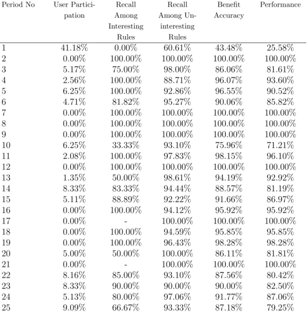
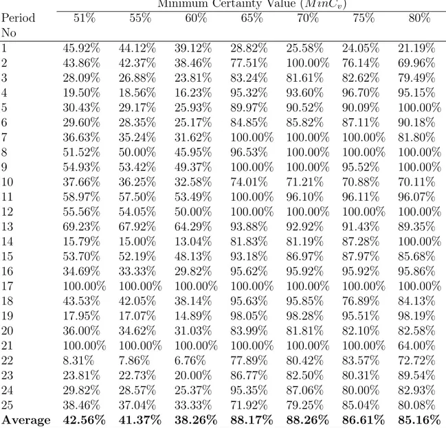
5.2 User Participation, Recall, Benefit Accuracy, and Performance values at MinCv = 70% . . . 75

5.3 Performance comparison at various minimum certainty values.

Friedman Test employed for significance test. Asymp.Sig. =

2.015e−18 _{at α = 0.05 . . . 76}

5.4 Comparison of BM IRIL against BM IRIL using the Naive

Bayesian classifier as the core classifier at MinCv = 70%.

Wilcoxon Test employed for significance test.

For Benefit Accuracy comparison criterion, Asymp.Sig.(2 −

tailed) = 1.229e−5 _{at α = 0.05}

For User Participation comparison criterion, Asymp.Sig.(2 −

tailed) = 1.228e−5 _{at α = 0.05}

For Performance comparison criterion, Asymp.Sig.(2−tailed) = 1.23e−5 _{at α = 0.05 . . . 77}

5.5 Comparison of BM IRIL against BM IRIL that does not use certainty on single feature prediction. Wilcoxon Test employed for significance test.

For Benefit Accuracy comparison criterion, Asymp.Sig.(2 −

tailed) = 0.03 at α = 0.05

For User Participation comparison criterion, Asymp.Sig.(2 −

tailed) = 0.006 at α = 0.05

For Performance comparison criterion, Asymp.Sig.(2−tailed) = 0.009 at α = 0.05 . . . 78 5.6 Comparison of BM IRIL against BM IRIL that does not use

in-stant concept update. Wilcoxon Test employed for significance test.

For Benefit Accuracy comparison criterion, Asymp.Sig.(2 −

tailed) = 0.001 at α = 0.05

For User Participation comparison criterion, Asymp.Sig.(2 −

tailed) = 0.001 at α = 0.05

For Performance comparison criterion, Asymp.Sig.(2−tailed) = 0.001 at α = 0.05 . . . 79

5.7 Comparison of BM IRIL against BM IRIL that does not use feature weighting. Wilcoxon Test employed for significance test. For Benefit Accuracy comparison criterion, Asymp.Sig.(2 −

tailed) = 0.433 at α = 0.05

For User Participation comparison criterion, Asymp.Sig.(2 −

tailed) = 0.331 at α = 0.05

For Performance comparison criterion, Asymp.Sig.(2−tailed) = 0.351 at α = 0.05 . . . 80

AQ15 : An incremental learner of attribute-based descriptions from examples

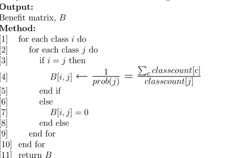
B : Benefit Matrix

Benef itAccuracyp: Benefit Accuracy at period p

BM IRIL : Benefit-Maximizing, Interactive Rule Interaction Learning algorithm BMCVFP : Benefit-Maximizing Classifier by Voting Feature Projections

c : Class

C4.5/C5.0 : An industrial-quality descendant of ID3

DBSCAN : Density-Based Spatial Clustering of Applications with Noise

FCLS : Flexible Concept Learning System

gpdf : Gaussian Probability Distribution Function

I : Item Set

ID3 : Iterative Dichotomiser 3 algorithm

KDD : Knowledge Discovery in Databases

KMEANS : Partitioning clustering algorithm

MinCv : Minimum Certainty Value Threshold

m(X) : Number of transactions containing or matching the set of items X ∈ I

N : Number of transactions

p : Period

r : Rule

R : Rule

Rp : Set of rules induced at period p

Rsp : Set of rules classified with sufficient certainty by BMCVFP at period p

Rt : Set of training rules

Rup : Set of rules classified by the user at period p

t : Training instance

T : Transaction

µ : Mean

σ : Standard deviation

Introduction

Data mining is the process of efficient discovery of patterns, as opposed to data itself, in large databases [16]. It encompasses many different techniques and algorithms. They differ in the kinds of data that can be analyzed and the kinds of knowledge representation used to convey the discovered knowledge. Patterns in the data can be represented in many different forms, including classification rules, association rules, clusters, sequential patterns, time series, contingency tables, and others [28]. In many domains, there is a continuous flow of data and therefore, learned patterns. This causes the number of patterns to be so huge that selection of the useful or interesting ones becomes difficult.

Selecting the interesting patterns among the induced ones is important because only a few of the total induced patterns are likely to be of any interest to the domain expert analyzing the data. The remaining patterns are either irrelevant or obvious, and do not provide any new knowledge.

To increase the utility, relevance, and usefulness of the discovered patterns, techniques are required to reduce the number of patterns. Some good metrics that measure the interestingness of a pattern are needed.

There are two aspects of pattern interestingness, objective and subjective aspects and this fact is what makes finding interesting patterns a challenging issue. Objective measures rate the patterns based on some statistics computed from the observed data. They are domain-independent and require minimal

user participation. On the other hand, subjective measures are user-driven; they are based on user’s belief in data, e.g., unexpectedness, novelty, and ac-tionability.

Both types of interestingness measures have some drawbacks. A particular objective interestingness measure is not sufficient by itself [41]. It may not be suitable on some domains. Authors in [33] investigate this issue and discover clusters of measures existing in a data set. An objective measure is gener-ally used as a filtering mechanism before applying a subjective measure. In the case of subjective interestingness measures, a user may not be competent in expressing his/her domain knowledge at the beginning of the interesting-ness analysis. Another drawback of a subjective measure is that the induced patterns are compared against the domain knowledge that addresses the unex-pectedness and/or actionability issues. Interestingness is assumed to depend only on these two factors. That is, if a pattern is found to be unexpected, it is automatically regarded as interesting.

It would be better to view unexpectedness and actionability as two of the interestingness factors and to develop a system that takes a set of interesting-ness factors into account to learn the interestinginteresting-ness concept of the induced patterns automatically with limited user interaction. The interaction can be realized by asking the user to classify some of the patterns as “interesting” or “uninteresting”.

Association rules are among the important pattern types and employed to-day in many application areas including web usage mining, intrusion detection, filtering, screening, and bioinformatics.

Let us give some preliminaries on association rules. Let I =

{item1, item2, . . . , itemn} be a set of items. Let S be a set of transactions,

where each transaction T ⊆ I. An association rule R is an implication of the form A → B, where A ⊆ I, B ⊆ I and A ∩ B = Ø, satisfying predefined support and confidence thresholds. Association rule induction is a powerful method for so-called market basket analysis, which aims at finding regularities in the shopping behavior of customers of supermarkets, mail-order companies and the like. In an association rule of the form R : A → B, A is called the

antecedent or body of the rule; B is called the consequent or head of the rule. A common application domain of association rules is sales data, known as basket data. In a typical application of association rule learning from market basket data, a set of transactions for a fixed period of time is used as input to rule learning algorithms. For example, the well-known Apriori algorithm can be applied to learning a set of association rules from such a transaction set. However, learning association rules from a set of transactions is not a one-time only process. For example, a market manager may perform the association rule learning process once every month over the set of transactions collected through the previous month. For this reason, it is worthwhile to consider the problem where transaction sets are input to rule learning algorithms as a stream of packages.

In this thesis, we deal with the interestingness issue of association rules discovered in domains from which information in the form of transactions is gathered at different time intervals.

The sets of transactions may come in varying sizes and in varying periods. That is, the number of transactions in a particular period may be quite different from those of the other periods. For example, if we think of the purchasing trends of customers, sales generally increase towards the end of the year and decrease in case of an economical crisis. Furthermore, it may not be possible to receive the transactions regularly. For example, if we think of a shopping center, there will not be any sales while the center is out of service, possibly for some constructional works.

Once a set of transactions arrives, the association rule learning algorithm is run on the last set of transactions, resulting in a new set of association rules. Therefore, the set of association rules learned will accumulate and increase in number over time, making the mining of interesting ones out of this enlarging set of association rules impractical for human experts. We refer to this sequence of rules as “streaming association rules” and the main motivation behind this research is to develop a technique to overcome the interesting rule selection problem.

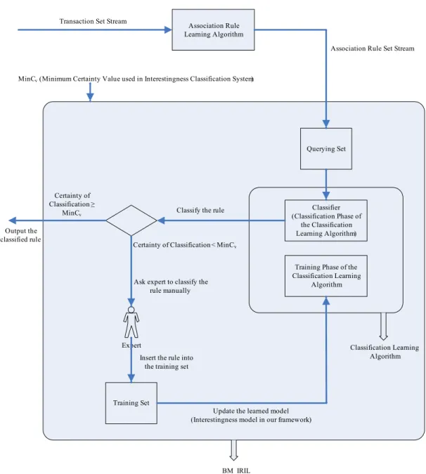
Expert Transaction Set Stream

Association Rule Learning Algorithm Querying Set Classifier (Classification Phase of the Classification Learning Algorithm)

Training Phase of the Classification Learning

Algorithm

Training Set

MinCv(Minimum Certainty Value used in Interestingness Classification System)

Certainty of Classification ≥

MinCv

Output the classified rule

Association Rule Set Stream

Classification Learning Algorithm Classify the rule

Certainty of Classification < MinCv

Ask expert to classify the rule manually

Insert the rule into the training set

Update the learned model (Interestingness model in our framework)

BM_IRIL

The definition of interestingness on a given domain usually differs from one expert to another and also over time for a given expert. The proposed system, “Benefit-Maximizing Interactive Rule Interestingness Learning” (BM IRIL) al-gorithm, learns a subjective model for the interestingness concept description of the induced rules. The interaction with the user ensures this subjectivity. It formulates the interestingness concept of streaming association rules as a benefit-maximizing classification problem and learns a different interestingness model for each user.

BM IRIL, whose schematic form is shown in Fig.1.1, is a post-processing

system that works in an incremental manner, employs a benefit-maximizing classifier inside, tries to classify the incoming rules with sufficient certainty and keeps user interactivity at a certain level.

BM IRIL was evaluated on a real supermarket dataset. We recorded the

customer transactions for 25 weeks. Each week is taken as the unit of period and has its own set of transactions. Following this, we induced association rules from the set of transactions for each period and used them as input to the BM IRIL algorithm.

A transaction set consists of transactions, and a transaction (in the super-market domain) contains the items bought by a customer at one swoop. An example transaction is:

{milk, egg, detergent, butter, coke, beer}

A transaction set belongs to a particular period, and association rules are learned from each of these sets. An example association rule is:

{tomato, cucumber, potato} → {lemon, onion}

Each association rule is regarded as a query instance and tried to be classi-fied by the inside classifier of the BM IRIL algorithm with sufficient certainty. If the classifier is not so certain to say “interesting” or “uninteresting” for the interestingness label of the association rule, user participation is put into use. The user evaluates the rule not only by looking at its content, but also by

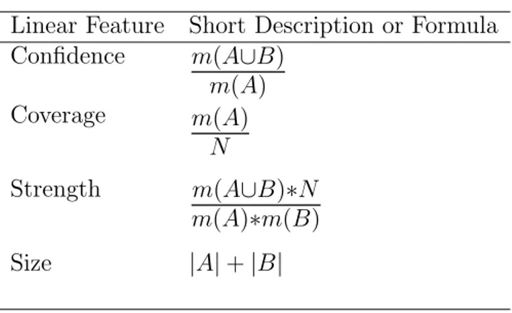
analyzing the objective factor values of this rule computed beforehand. The objective factors used in this dissertation are confidence, coverage, strength, and size. Each selected objective factor carries information about a specific property of the association rules. These are accuracy, applicability, indepen-dency, and simplicity properties of the association rules, respectively. The details about the computation of these factors are given in Chapter 4.

Once the user evaluates a rule as “interesting” or “uninteresting”, this rule becomes a training instance for the inside classifier of the BM IRIL algorithm, and the interestingness model is updated. The inside classifier proposed in this dissertation is a feature projections based classifier. It employs confidence, coverage, strength, size, and the rule’s content itself as the determining fea-tures. The learned model is the combination of the local models learned on each feature projection.

An example of a learned interestingness model is: if the confidence > 70% → rule is interesting if the coverage > 50% → rule is interesting if the strength < 1 → rule is uninteresting if the size of the rule > 6 → rule is uninteresting

if the antecedent of the rule is similar to {milk, egg} → rule is uninteresting (user is not interested in rules containing milk and egg in the body part of the rule)

if consequent of the rule is similar to {beer} → rule is interesting (user is interested in rules containing beer in the head part of the rule. He would like to know which items lead to the sales of beer)

if the rule is similar to ({tomato} → {cucumber}) → rule is uninteresting (user is not interested in rules containing such a trivial implication)

1.1

Contributions

The contributions of this dissertation can be listed as follows:

• modeling the interestingness concept of association rules as a

classifica-tion problem and proposing an active learning approach (BM IRIL) for this purpose,

• suitability of the BM IRIL approach for domains where enormous amount

of transactions arrives in varying time periods,

• learning the interestingness model rather than using a given

interest-ingness model that addresses only unexpectedness and/or actionability aspects of association rules,

• selecting both objective and subjective interestingness factors of

associa-tion rules as determining features in modeling the interestingness concept as a classification problem,

• handling the unexpectedness and actionability subjective interestingness

factors by proposing a new feature type, ordered-pair of sets. This new feature type is quite different from the classical linear and nominal feature types that are already in use by the machine learning community,

• proposing a new classifier suitable to work with ordered-pair of sets type

features,

• learning user specific interesting rules rather than the generic interesting

rules.

1.2

Outline of the Thesis

In the next chapter, we review the data mining techniques briefly and highlight the interestingness concept defined to overcome the huge number of patterns induced as a result of the mining process. In Chapter 2, we also review the categorization of the interestingness measures and give numerous examples in

the literature. In this thesis, we propose a method that has the ability to formulate the interestingness issue of association rules as a benefit-maximizing classification problem. Therefore, it makes sense to choose an appropriate classifier to be used in the proposed method. Chapter 3 is devoted to the choice of an appropriate benefit-maximizing classifier. Upon selection of an appropriate classifier, modeling interestingness of streaming association rules as a benefit-maximizing classification problem is explained in Chapter 4. Giving the empirical evaluations in Chapter 5, we conclude the thesis with Chapter 6.

Previous Work

Data mining encompasses many different techniques and algorithms. They differ in the kinds of data that can be analyzed and the kinds of knowledge representation used to convey the discovered knowledge. In this chapter, we review these techniques briefly and highlight the interestingness concept defined to overcome the huge number of patterns induced as a result of the mining process. We also review the categorization of the interestingness measures and give numerous examples in the literature.

2.1

Basic Data Mining Techniques

Knowledge discovery in databases (KDD) refers to the overall process of dis-covering useful knowledge from data, and data mining refers to a particular step in this process [16]. KDD involves many steps including data prepara-tion, data selecprepara-tion, data cleaning, incorporation of appropriate prior knowl-edge, data mining and proper interpretation of the results of mining. The data mining step is the efficient discovery of previously unknown, valid, interesting, novel, potentially useful, and understandable patterns in large databases. The knowledge that we seek to discover describes patterns in the data as opposed to knowledge about the data itself. Patterns in the data can be represented in many different forms, including classification rules, association rules, clusters,

sequential patterns, time series, contingency tables, summaries obtained using some hierarchical or taxonomic structure, and others [28].

2.1.1

Classification

Classification is perhaps the most commonly applied data mining technique. Early examples of classification techniques from the literature include Quinlan’s ID3 [58], Michalski et al.’s AQ15 [48] and Naive Bayes Classifier [30]. ID3 induces a decision tree. An object is classified by descending the tree until a branch leads to a leaf node containing the decision. AQ15 induces a set of decision rules. An object is classified by selecting the most preferred decision rule according to user-defined criteria. Naive Bayes Classifier’s approach to classifying the new instance is to assign the most probable target value, given the predicting attribute values that describe the instance. Later examples of classification techniques from the literature include Zhang and Michalski’s FCLS [71], and Quinlan’s C4.5/C5.0 [59]. FCLS induces a weighted threshold rule. The threshold determines the number of conditions that must be satisfied in a valid rule. An object is classified by generalizing and specializing examples until the number of incorrectly classified examples is below some user-defined error rate. C4.5/C5.0 is an industrial-quality descendant of ID3 that has seen widespread use in the research community.

2.1.2

Association

Association is another commonly applied data mining technique. The prob-lem is typically examined in the context of discovering purchasing patterns of customers from retail sales transactions, and is commonly referred to as market basket analysis. The association task involves the discovery of knowl-edge with a user-defined accuracy (confidence factor) and relative frequency (support factor).

Much of the literature focuses on the Apriori algorithm [1] and its descen-dants containing various refinements and improvements. Apriori extracts the

set of frequent itemsets from the set of candidate itemsets generated. A fre-quent itemset is an itemset whose support is greater than some user-defined minimum and a candidate itemset is an itemset whose support has yet to be determined. It has an important property that if any subset of a candidate itemset is not a frequent itemset, then the candidate itemset is also not a frequent itemset.

2.1.3

Clustering

Clustering, also a frequently used data mining technique, is the process of identifying objects that share some distinguishing characteristics. There are numerous techniques of clustering in the literature.

A well-known example of clustering in the literature is the k-means algo-rithm [31]. Given a set of objects X and an integer number k, the k-means algorithm searches for a partition of X into a predefined k number of clusters that minimizes the inter-cluster distance of squared errors and maximizes the intra-cluster similarity measure.

More recent examples from the literature include DBSCAN [15] by Ester et al. DBSCAN is a density-based approach that utilizes user-defined parameters for controlling the density of the discovered clusters. This approach allows adjacent regions of sufficiently high density to be connected to form clusters of arbitrary shape and is able to differentiate noise in regions of low density.

2.1.4

Correlation

Correlation is a statistical measurement of the relationship between two vari-ables. Possible correlations range from “+1” to “-1”. A zero correlation in-dicates that there is no relationship between the variables. A correlation of “-1” indicates a perfect negative correlation, meaning that as one variable goes up, the other goes down. A correlation of “+1” indicates a perfect positive correlation, meaning that both variables move in the same direction together.

Statistically oriented in nature, correlation has also seen increasing use as a data mining technique. Even though the analysis of multi-dimensional categorical data is possible, the most commonly employed method is that of two-dimensional contingency table analysis of categorical data using the chi-square statistic as a measure of significance [67].

2.1.5

Summarization

Summarization involves the discovery of high-generality knowledge, i.e. a dis-covered rule should cover a large amount of data (which is not the main re-quirement of other tasks such as classification).

In the summarization task, the goal is to produce some characteristic de-scription of a class. This dede-scription is a kind of summary, describing some properties shared by all (or most) tuples belonging to that class. In the case of discovered summaries expressed in the form of rules, the discovered rules can be interpreted in the following way: “If a tuple belongs to the class indicated in the antecedent of the rule, then the tuple has all the properties mentioned in the consequent of the rule”. Hilderman and Hamilton give various heuristic measures of interestingness for summarization task [27]. These measures in-clude Simpson, Shannon, Theil, Atkinson, etc. A characteristic rule does not aim at discriminating classes, as classification rules do. This stems from the fact that a characteristic rule for a given class is produced by taking into ac-count only tuples belonging to that class. This is in contrast with classification rules, where each rule is produced by taking into account tuples belonging to different classes.

Classification, regression and summarization can be regarded as a form of supervised discovery, since the user specifies the goal attribute (or class attribute) and the system has to discover some relationship between that at-tribute and the other atat-tributes. However, unsupervised learning tasks can be transformed into supervised ones by the user, if this is convenient (e.g. by spec-ifying the constraint that a given goal item be the only item in the consequent of an association rule).

2.2

Interestingness Concept

Typically, the number of patterns generated by the data mining techniques is very large, but only a few of these patterns are likely to be of any interest to the domain expert analyzing the data. The reason for this is that many of the patterns are either irrelevant or obvious, and do not provide any new knowledge. To increase the utility, relevance, and usefulness of the discovered patterns, techniques are required to reduce the number of patterns that are necessary to be considered. In order to satisfy this goal, some good metrics that measure the interestingness of a pattern are needed.

A pattern is interesting if it is easily understood, unexpected, potentially useful and actionable, novel, or it validates some hypothesis that a user seeks to confirm. There are two aspects of pattern interestingness, objective and subjective aspects and this fact is what makes finding interesting patterns a challenging issue. Objective measures rate the patterns based on some statis-tics computed from the observed data. They include measures such as sup-port, confidence, chi-square, and correlation. Objective measures are domain-independent and require minimal user participation (aside from specifying the quality measure threshold). Some objective measures are symmetric with re-spect to permutation of the items while others are not. From an association rule mining perspective, symmetric measures are often used for itemsets whereas asymmetric measures are applied to rules. These measures can be applied dur-ing mindur-ing or post-processdur-ing steps of the knowledge discovery process. On the other hand, subjective measures are user-driven; they are based on user’s belief in data, e.g., unexpectedness, novelty, and actionability.

Interesting patterns should be selected among the generated ones. Although there are several studies on this subject, there is not a standard or universally best measure to decide which pattern is interesting or which one is not, yet.

B ¬B

A f11 f10 f1+

¬A f01 f00 f0+

f+1 f+0 N

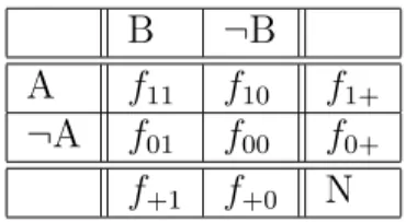
Table 2.1: 2 x 2 contingency table for binary variables

2.2.1

Objective Measures From Statistics

2.2.1.1 Goodness of fit test

This class of methods compare the actual distribution of a data set to its expected distribution under a null hypothesis. To test for item dependence, the null hypothesis assumes that a pattern consists of items that are independent of each other. Then, based on evidence provided by the observed data, one can determine whether to accept or reject the independence assumption. Although this class of methods are good, the techniques that directly estimate the degree of dependence are often more desirable.

To illustrate the test, let A and B denote a pair of binary variables. The data set that contains these variables can be summarized into a 2x2 contingency table as shown in Table 2.1. Each cell represents the four possible combinations of A and B values. fij corresponds to the frequency (support count) for each

cell; while fi+ = fi0+ fi1 and f+j = f0j+ f1j . Also, N refers to the size of the

database.

Pearson’s χ2 _{statistic is often used for goodness of fit test:}

χ2 ₌X j,k (fo jk− fjke )2 fe jk

This statistic measures the sum of the normalized deviation between the ob-served support count, fo

jk, of each cell in the contingency table from its expected

support count, fe

jk. To test for variable dependencies, it is first hypothesized

that the variables are independent of each other. In this case, the expected support count for each contingency table cell entry is fe

jk = N( fo j+ N )( fo +k N ). For

the 2x2 contingency table shown in Table 2.1, its χ2 _{value can be simplified}

into the following expression:

χ2 ₌ N(f11f00− f01f10)2

f1+f0+f+1f+0

If the computed χ2 _{value is large, then we have more evidence to reject the}

independence hypothesis. This begs the question of how large should the χ2

value be in order to conclude with high confidence that the variables are not independent? By looking up the standard probability tables for χ2_{distribution,}

a cutoff value can be obtained for which the independence assumption can be rejected at any significance level α.

However, χ2 _{does not tell us the strength of correlation between items in}

an association pattern. Instead, it will only help us to decide whether items in the pattern are independent of each other. Thus, it cannot be used for ranking purposes. Another disadvantage is that the χ2 _{statistic depends on}

the total number of transactions. But, the χ2 _{cutoff value depends only on}

the degrees of freedom of the attributes, (which is one for binary attributes) and the significance level desired. For example, the rejection region for binary attributes at 0.05 significance level is 3.84. When the number of transactions is large, the cutoff value can be exceeded by a very large number of itemsets.

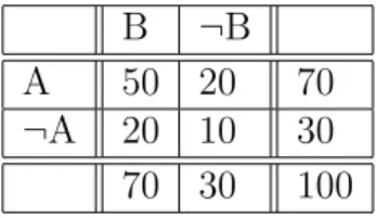
2.2.1.2 Correlation Coefficient

In statistics, a standard way to measure the degree of association between binary variables is to use Pearson’s φ-coefficient, where

φ = pf11f00− f10f01

f1+f0+f+1f+0

The value of this coefficient ranges from -1 to +1. φ-coefficient is desir-able because it relates to statistical correlation, a widely accepted measure in statistics. However, it is also symmetric in terms of exchanging f11↔ f00 and

large f00 from large f11. For example, Table 2.2 should correspond to a more

interesting pattern compared to the one in Table 2.3, yet their φ-coefficients stay the same, since Table 2.2 has a larger support.

B ¬B

A 50 20 70

¬A 20 10 30

70 30 100

Table 2.2: A 2 x 2 contingency table of a more interesting pattern

B ¬B

A 10 20 30

¬A 20 50 70

30 70 100

Table 2.3: A 2 x 2 contingency table of a less interesting pattern Other measures from statistical literature include Goodman and Kruskal’s λ and τ coefficients, Pearson’s coefficient of contingency, uncertainty coefficients, etc [67].

2.2.2

Objective Measures From Data Mining

2.2.2.1 Support and Confidence

A rule A → B has support s if s% of all the transactions contains both A and B. The rule has a confidence c if c% of all transactions that contain A also contains B. Those rules that exceed a predetermined minimum threshold for support and confidence are considered to be interesting. Since the choice of an appropriate support threshold is often ad-hoc, it should be ensured that support-based pruning would not remove many of the interesting patterns. Ku-mar et al. [67] indicate that placing a maximum support threshold will lead to pruning uncorrelated, positively correlated and negatively correlated itempairs in equal proportions to their initial distribution. In contrast, if a minimum support threshold is specified, most of the itempairs removed are either uncor-related or negatively coruncor-related [67]. But, if the minimum support threshold is

too high, it tends to produce patterns that are obvious to most analysts. On the other hand, a low minimum support threshold may result in an unmanage-able number of patterns. Furthermore, some of the most interesting patterns may have very low support, e.g. patterns involving expensive jewelries. Cur-rently, there have been some attempts to rectify this problem such as assigning weights to different items [8], using a relative interestingness measure [32] or employing a combination of random sampling and hashing techniques [12] to mine exception rules. Hussain et al. argue that objective measures are al-ways reliable due to their unbiased nature, but those measures are sometimes completely unable to justify a rule’s interestingness as they can not handle knowledge from common sense rules [32]. The example below illustrates the situation:

A → X Common Sense Rule (Strong Pattern) (High support, high confidence)

A, B → ¬X Exception Rule (Weak Pattern)

(Low support, high confidence)

B → ¬X Reference Rule

(Low support and/or low confidence)

Hussain et al. search for reliable exceptions starting from the common sense rules [32]. They find exception rule from the two common sense rules

A → X and B → X (B → X as common sense infers B → ¬X to be reference

for its obvious low support and/or low confidence). By doing this, they can estimate the amount of surprise the exception rule brings from the knowledge of extracted rules. If only the above exception rule were given, it would not be objectively interesting. However, if the other two common sense rules (A → X and B → X) are known then the exception rule should be interesting. This suggests a need to have a relative interestingness measure. That is, Hussain et al. mine rules that are objectively interesting, but in the meantime they measure interestingness with respect to already mined rules.

Cohen et al. state that Apriori algorithm is only effective when the only rules of interest are relationships that occur very frequently [12]. However, there are some applications, such as identification of similar web documents, where the rules of interest have comparatively few instances in the data. In these cases, we must look for highly correlated items, or possibly even causal

relationships between infrequent items. Cohen et al. develop a family of algo-rithms for solving this problem, employing a combination of random sampling and hashing techniques [12].

Since support is an objective measure, it does not involve domain knowl-edge. Incorporating domain knowledge may require having an subjective inter-estingness measure. Sarawagi et al. propose using temporal description length to approximate the role of domain knowledge in the search for interesting pat-terns [10]. They concentrate on the problem of boolean market basket data and states that a set of k items is interesting, not necessarily because its sup-port exceeds a user-defined threshold, but because the relationship between the items changes over time and these changes are not totaly explained by the changes in the support of smaller subsets of items. Sarawagi et al. propose a precise characterization of surprise based on the number of bits in which a basket sequence can be encoded under a carefully chosen coding scheme [10]. In this scheme, it is inexpensive to encode sequences of itemsets that have steady, hence likely to be well known, correlation between items. Conversely, a sequence with large code length hints at a possibly surprising correlation.

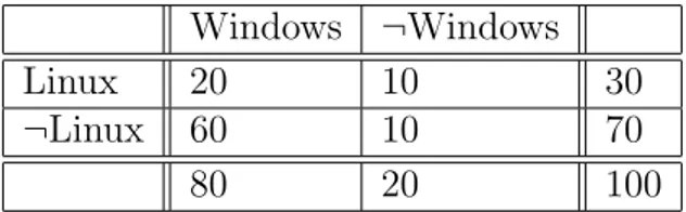
The Confidence measure can be misleading in some situations, as explained in the following example.

Windows ¬Windows

Linux 20 10 30

¬Linux 60 10 70

80 20 100

Table 2.4: A 2 x 2 contingency table example pointing out a situation where confidence is misleading

Suppose the support and confidence thresholds were set at 5% and 50%, respectively. The association rule Linux → Windows would have a 20% support and 67% confidence. Thus, it will pass both threshold conditions and eventually declared to be interesting. However, this information is misleading. The prior probability that a customer buys Windows is 80%. Once it is known that the customer had bought Linux, the conditional probability that he or she would buy Windows reduces to 67%. In other words, the discovered rule does not

make sense. This is why confidence may not be an appropriate measure. If it is assumed that the overall confidence of an itemset is represented by the maximum confidence among the rules that can be generated from this itemset, it is observed that there is a linear relationship between Pearson’s

φ -coefficient and the overall confidence in the range of typically encountered

support values. In fact, the most interesting rule according to any objective measure must reside along a support border [5].

2.2.2.2 Interest Factor

The Interest factor is another objective measure of association between items [67]. It is defined as the ratio between the joint probability of two items to their marginal probabilities:

I(X, Y ) = P (X, Y ) P (X)P (Y ) =

f11N

f1+f+1

This ratio can range anywhere between 0 and +∞ . An interest factor of 1 corresponds to total independence between the two items. Positively (or negatively) correlated items will have an interest factor greater (less) than 1. Unfortunately, this measure can be close to one (independence) even though the two items are highly dependent on each other. For example, let’s consider the following situation: Let P(X,Y) = 0.1, P(X) = 0.1 and P(Y) = 0.1. The interest factor is large i.e., 1 / 0.1 = 10, while its φ-coefficient is equal to 1 (perfect positive correlation). Now, if P(X,Y) = 0.9, P(X) = 0.9 and P(Y) = 0.9, once again the φ-coefficient is equal to 1. However, the interest factor has dropped dramatically from 10 to 1 / 0.9 = 1.11, which is very close to the independence situation.

This objective measure also has a linear relationship (strong correlation) with φ-coefficient in the range of typically encountered support values [67].

2.2.2.3 Conviction

The Conviction measure is proposed as an alternative to interest factor be-cause they needed an asymmetric objective measure for implication rules [67]. Conviction is defined to be:

conviction = P (X)P (¬Y ) P (X, ¬Y )

This measure is derived from interest factor in the following way. A rule

X → Y is logically equivalent to ¬(X ∩ ¬Y ). Thus, above equation is an

asymmetric way for testing independence between X and Y . The ratio between

P (X, ¬Y ) and P (X)P (¬Y ) is inverted due to the negation symbol in the logical

expression ¬(X ∩ ¬Y ).

Conviction is different from confidence because it does not suffer from the problem of producing misleading rules. Unlike interest factor, conviction will assign the value +∞ if the confidence of the rule is 1 (regardless of what

P (X, Y ) is). If two items are independent, their conviction value will be equal

to 1.

2.2.2.4 Gini Index

For an association rule of the form X → Y , Gini [67] is defined as follows:

Gini = P (X)(P (Y |X)2_{+ P (¬Y |X)}2_{) + P (¬X)(P (Y |¬X)}2_{+ P (¬Y |¬X)}2₎

− P (Y )2− P (¬Y )2

The values for the Gini index range between 0 (when the two items are independent) and 0.5 (when the two items are perfectly correlated). Gini index treats both positively and negatively correlated itemsets in the same way. However, as the range of support values is restricted, the negatively correlated pairs are eliminated.

2.2.2.5 Piatetsky-Shapiro’s rule-interest Piatetsky-Shapiro’s rule-interest is defined as:

RI = P (X, Y ) − P (X)P (Y )

The range of this measure is between -0.25 and 0.25. If X and Y are independent, RI = 0. RI is maximum when P (X, Y ) = P (X) = P (Y ) = 0.5. This measure also has a strong correlation with φ-coefficient in the range of typically encountered support values.

2.2.2.6 Entropy (Information Gain Ratio)

Entropy is developed from information theory and is defined for a rule X → Y as follows [67]:

Entropy = HX + HY − HXY HX

where

HX = −P (X) log P (X) − P (¬X) log P (¬X),

HY = −P (Y ) log P (Y ) − P (¬Y ) log P (¬Y ) and

HXY =

P

i

P

jP (X = i, Y = j) log P (X = i, Y = j).

The range of this measure is between 0 (for absolute independence) and 1 (for perfect correlation). This measure treats positive and negatively correlated items in the same way.

2.2.2.7 Neighborhood-based Unexpectedness

Dong and Li introduce neighborhood-based interestingness by considering un-expectedness in terms of neighborhood-based parameters [14]. They first

present some novel notions of distance between rules and of neighborhoods of rules. The neighborhood-based interestingness of a rule is then defined in terms of the pattern of the fluctuation of confidences or the density of the mined rules in some of its neighborhoods. They rank the interesting rules by com-bining some neighborhood-based characteristics, the support and confidence of the rules, and user’s feedback.

Taking the association rules into account, we might think that it is possible to handle the post-mining rule analysis problem by increasing the threshold values. This way, the number of induced association rules will decrease. How-ever, using the world map analogy, only those global peaks will be induced and the useful information conveyed by those local peaks over vast plains will be missed [14]. For example, suppose we have two different geographical regions A and B, where A is a mountainous area with an average altitude of 5000 meters and B is a vast plain with an average altitude of 50 meters. A mountain with a height of 6000 meters in A is not as interesting as a mountain with a height of 1000 meters in B. That is, the interestingness concept should also be related to the position among neighborhoods.

Interestingness is used to evalute the importance of an association rule by considering its unexpectedness in terms of other association rules in its neigh-borhood. The neighborhood of an association rule consists of all association rules within a given distance. The distance metric is given by:

D(R1, R2) = δ1|(X1∪ Y1)Θ(X2∪ Y2)| + δ2|X1ΘX2| + δ3|Y1ΘY2|

where R1 = X1 → Y1, R2 = X2 → Y2, δ1, δ2 and δ3 are parameters to

weight the relative importance of all three terms, and Θ is an operator denoting the symmetric difference between X and Y (i.e.,(X − Y ) ∪ (Y − X)). An r-neighborhood of a rule is given by the set:

N(Ro, r) = {R|D(R, Ro) ≤ r, R a potential rule}

and is used to define the interestingness of a rule. Two types of interestingness are unexpected confidence and isolated interestingness. Unexpected Confidence

Interestingness is given by: UCI =    1 if ||c(Ro) − ac(Ro, r)| − sc(Ro, r)| > t1 0 otherwise

where c(Ro) is the confidence of Ro, ac(Ro, r) and sc(Ro, r) are the average

confidence and standard deviation of the confidences of the rules in the set

M ∩ N(Ro, r) - {Ro} (M is the set of rules satisfying the minimum support

and confidence), and t1 is a threshold.

II =    1 if |N(Ro, r)| − |M ∩ N(Ro, r)| > t2 0 otherwise

where |N(Ro, r)| is the number of potential rules in an r-neighborhood, |M ∩

N(Ro, r)| is the number of rules generated from the neighborhood, and t2 is a

threshold.

2.2.3

Subjective Measures

One approach to defining interestingness of a pattern is to define it in objective terms, where interestingness of a pattern is measured in terms of its structure and the underlying data used in the discovery process. However, that objective measures of interestingness, although useful in many respects, usually do not capture all the complexities of the pattern discovery process, and are not suf-ficient in many data mining applications because one can still generate a large number of strong rules that are interesting “objectively” but of little interest to the user. Thus, subjective measures of interestingness are needed to define interestingness of a pattern.

2.2.3.1 Silberschatz’s Belief System

The subjective measures do not depend only on the structure of a rule and on the data used in the discovery process, but also on the user who examines the pattern [64]. These measures recognize that a pattern that is of interest to one

user, may be of no interest to another user. There are two major reasons why a pattern is interesting from the subjective (user-oriented) point of view:

• Actionability Measure

A pattern is interesting if the user can do some action after he/she sees the pattern. The user can use the outcomes of the interesting pattern to his/her advantage. Actionability is an important subjective measure of interestingness because users usually prefer to see the knowledge that makes their lives easy, by taking proper actions in response to the newly discovered and learned patterns.

• Unexpectedness Measure

Unexpectedness measure can be analyzed both objectively and subjec-tively. A newly discovered pattern can be surprising to the user, which automatically leads it to be an interesting pattern. Surprising or un-expected patterns are interesting since they contradict expectations of the human beings, and the expectations naturally depend on the belief system. It is therefore convenient to define the unexpected measure of interestingness in terms of the belief system that the user owns. Silber-schatz et al. express interestingness of a pattern in terms of how it affects the belief system [64].

Unexpectedness and actionability are two different types of interesting-ness. There are patterns that are unexpected but non-actionable. There are patterns that are actionable but expected. There are also patterns that are both unexpected and actionable. It is worthwhile to note that most of the actionable patterns are also unexpected; and most of the unexpected patterns are also actionable [64]. Therefore, unexpectedness and actionability are good substitutes for each other.

Although both actionability and unexpectedness are important, people are usually interested in actionability since they prefer to react to the patterns to make their lives easy. However, actionability is very difficult to capture formally [64] because the space of all patterns should be par-titioned into a finite number of equivalence classes and a proper set of actions should be associated with each equivalence class. The space of all patterns is usually unknown in many situations. Even if the space

is known, it is a very hard task to partition the space into equivalence classes and to associate a proper set of actions with each equivalence class. Even if the space partitioning and the action associating steps suc-ceed, there is no guarantee that the actions and the association of the actions to the equivalence classes will never change. These difficulties make actionability difficult to capture formally.

Unexpectedness and actionability are good substitutes for each other. Most of the unexpected patterns are actionable and most of the action-able patterns are unexpected. Therefore, we can handle actionability through unexpectedness [64]. Unexpectedness is related to beliefs and beliefs are classified into two categories:

– Hard beliefs are beliefs that can never be changed despite contra-dictory evidence.

– Soft beliefs are beliefs that a user is willing to change if compelling new evidence are found.

Interestingness determines the extent to which a soft belief is changed as a result of encountering new evidence (i.e., discovered knowledge). A pattern is interesting relative to some belief system if it affects this system, and the more it affects it, the more interesting the pattern is. Interestingness within the context of soft beliefs is given by:

I =X

α

P (α|E, ²) − P (α|²) P (α|²)

where α is a belief, E is new evidence, ² is the previous evidence sup-porting belief α, P (α|²) is the confidence in belief α, and P (α|E, ²) is the new confidence in belief α given the new evidence E. Summation is over all beliefs. The Bayes theorem is used to determine the new confidence and is given by:

P (α|E, ²) = P (E|α, ²)P (α|²)

P (E|α, ²)P (α|²) + P (E|¬α, ²)P (¬α|²)

The Bayesian approach can be applied to arbitrary beliefs not only for beliefs expressed as rules [64].

2.2.3.2 Liu’s Fuzzy Matching Technique for Classification Rules Rule induction research implicitly assumes that after producing the rules from a data set, these rules will be used directly by an expert system or a human user. In real-life applications, the situation may not be as simple as that, particularly, when the user of the rules is a human being. The human user almost always has some previous concepts or knowledge about the domain represented by the data set. Naturally, he/she wishes to know how the new rules compare with his/her existing knowledge [41]. With the increasing use of machine learning techniques in practical applications such as data mining, this issue of post-analysis of rules warrants greater emphasis and attention. Liu and Hsu perform the post-analysis of classification rules generated by systems such as C4.5. They propose a fuzzy matching technique to perform the post-analysis of classification rules [41].

Most of the work on machine learning focuses on the generation of rules from various types of data sets as well as pruning of the generated rules [59, 7]. Some systems also use existing domain knowledge in the induction process [53, 11, 57]. However, their purpose is mainly for helping the induction process so as to increase learning efficiency and/or improve prediction accuracy of the generated rules. Clearly, the focus of their research is quite different from the one presented by Liu and Hsu, which is primarily a post-analysis method that aims to help the user analyze the rules generated.

In the fuzzy matching technique developed to perform the post-analysis of rules, existing rules, E, (from previous knowledge) are regarded as fuzzy rules and are represented using fuzzy set theory. The newly generated rules, B, are matched against the existing fuzzy rules using the fuzzy matching technique. The matching process results in identifying conforming and unexpected rules. They present a high level view of the fuzzy matching method. It consists of two main steps:

• The user converts each rule in E to a fuzzy rule. The fuzzy rule has

the same syntax as the original rule, but its attribute values must be described using some fuzzy linguistic variables.

• The system matches each new rule Bi ∈ B against each fuzzy rule Ej ∈ E

in order to obtain the degree of match for each new rule Bi against the

set E. The new rules in B are then ranked according to their degrees of match with E.

The rules in E and B have the same syntax and semantics as the rules produced by C4.5. The syntax of the rules generated by C4.5 has the following form:

P1, P2, ..., Pn→ C

where “,” means “and”, and Pi is a proposition of the form: attr OP value,

where attr is the name of an attribute in the data set, value is a possible value for attr, and OP ∈ {=, 6=, <, >, ≤, ≥} is the operator. C is the consequent of the form: Class = value.

2.2.3.3 Liu’s Tuple-level Fuzzy Matching Technique for

Classifica-tion Rules

The technique proposed by Liu et al. asks the user to provide his/her ex-pected patterns according to his/her past knowledge and/or intuitive feelings [43]. Given these expectations, the system uses a tuple-level fuzzy matching technique to analyze and rank the discovered patterns according to a number of interestingness measures. In this technique, a number of rankings can be performed for different purposes. Two main types of ranking are conformity ranking and unexpectedness ranking.

The conformity can be measured at the pattern-level and at the tuple-level. Liu and Hsu propose a pattern-level fuzzy matching technique [41]. For example;

Discovered pattern (or rule): If X > 9, Y < 5, Q=2 Then R = TRUE User-expected pattern (or rule): If X > 9, Y < 6, P=4 Then R =TRUE

On the surface, the two rules seem similar (or conforming). The pattern-level match method in [41] will give a high conforming match value. However, it may be the case that tuples in the database suggest that (X>9, Y<5, Q=2) implies (X>9, Y<5, P=4) -the two patterns are conforming, or that (X>9, Y<5, P=4) implies R = FALSE -the user expected pattern is actually false, or other possible situations. Without consulting the actual database, it cannot be decided which one of these cases is true. However, it is obvious that pattern level matching is efficient.

2.2.3.4 Liu’s General Impressions for Classification Rules

Liu et al. propose a technique that analyzes the discovered classification rules against a specific type of existing knowledge, which they call general impres-sions, to help the user identify interesting rules [42]. They first propose a rep-resentation language to allow general impressions to be specified. They then present some algorithms to analyze the discovered classification rules against a set of general impressions. The results of the analysis tell us which rules conform to the general impressions and which rules are unexpected. Although both unexpected and conforming rules are considered to be interesting, unex-pected rules are more interesting.

Liu and Hsu report a fuzzy matching approach to analyze the discovered rules against the user’s existing concepts [41]. One limitation of this technique is that too much reliance is being placed on the user’s ability to supply the set of fuzzy expectations. In many situations, users do not know enough about their domains to supply the expected rules. Instead, Liu and Hsu find that even if the users cannot supply the set of fuzzy expectations, they do have certain general impressions (GI) about their domains [42]. Silberschatz et al. propose to use a belief system to describe unexpectedness [64]. However, this approach requires the user to provide complex belief information, such as conditional probabilities, which are difficult to obtain in practice. It does not handle GIs. Assume a human user has some previous concepts about the domain rep-resented by the database D. These concepts can be correct, partially correct or entirely wrong. Two types of existing concepts exist:

• General Impressions (GI): The user does not have detailed concepts

about the domain, but does have some vague feelings. For example, in a housing loan domain, the user may feel that having a high monthly salary increases one’s chance of obtaining a loan.

• Reasonably Precise Knowledge (RPK): The user has more definite

idea. For example, in the same loan domain, the user may believe that if one’s monthly salary is over $5000; one will be granted a loan. Of course, the user may not be so sure that it is exactly $5000. There is a fuzziness surrounding the value $5000 in his/her mind.

Liu and Hsu study the rule analysis against RPK [41], where as Liu et al. focus on GIs [42]. In the situation where one has some RPK about certain aspects of the domain, but only GIs about the others, a combined approach may be used.

Liu et al. analyze classification rules produced by C4.5 [42], as in the work described in [41]. A general impression is used to evaluate the importance of classification rules by comparing discovered rules to an approximate or vague description of what is considered to be interesting. So, a general impression is a kind of specification language. There are two types of general impressions that can be specified: Type 1 and Type 2.

A Type 1 general impression is a rule of the form A1OP1, A2OP2...AxOPx →

Cj, where each AiOPi is called an impression term, each Ai is an attribute,

each OPi is an impression descriptor from the set {<, >, <<, |, ¤}, and Cj

is a class. The < (>) impression descriptor means smaller (larger) attribute values are more likely to lead to inclusion in class Cj, << means some range

of attribute values are more likely to lead to inclusion in class Cj, | means

some relationship exists between an attribute and class Cj but the nature of

this relationship is not exactly known, and ¤ means that some subset of the possible values for an attribute are more likely to lead to inclusion in class Cj.

A Type 2 general impression is specified when there is more confidence that the combination of impression terms will lead to inclusion in class Cj.

AmOPm, AnOPn...AxOPx → Cj, where the part to the left (right) of the &

symbol is called the core (supplement). The core must always exist, otherwise the general impression should be specified as Type 1. If the supplement exists, then the rule is called a maximal impression. In a maximal impression, the general impression is that the impression terms in the core and any subset of those in the supplement are more likely to lead to inclusion in class Cj. If

the supplement does not exist, then the rule is called an exact impression. In an exact impression, the general impression is that the impression terms in the core are more likely to lead to inclusion in class Cj. The specified general

impressions are matched against the rules generated, and ranked to identify those that are most valid [42].

2.2.3.5 Rule Templates for Association Rules

Klemetinen et al. show how a formalism of rule templates makes it possible to easily describe the structure of interesting rules [37]. They also give examples of visualization of rules, and show how a visualization tool interfaces with rule templates. Templates, which are closer to regular expressions, can be used to describe the form of interesting rules, and also to specify which rules are not interesting.

For a rule to be presented to the user, a rule must be interesting; i.e., it should match one of the inclusive templates and it must not be uninteresting; i.e., it should not match with any of the restrictive templates [37]. That is, to be interesting, a rule has to match an inclusive template. If a rule, however, matches a restrictive template, it is considered as uninteresting. Rule pruning can be done by setting support, confidence, and rule size thresholds. But, although rule pruning based on support and confidence thresholds is effective, it fails to take into account special interests or domain knowledge. So, subjective measures such as rule templates provide effective solutions. The simple idea of classifying the attributes of the original data set to an inheritance hierarchy, and using templates defined in terms of that hierarchy, can be used to prune the rule sets effectively and according to the user’s intuitions. The drawback of rule templates is that the degree of interestingness is not specified [37]. To

Food Item

Fruit Dairy-Product Meat

grape pear apple milk cheese butter beef _chicken

Figure 2.1: A Taxonomy Example

give an interestingness value to the discovered rules, inclusive templates could be given weights.

2.2.3.6 Liu’s General Impressions, Reasonably Precise Concepts

and Precise Knowledge for Association Rules

Liu et al. propose a new approach to assist the user in finding the interest-ing rules (in particular, unexpected rules) from a set of discovered association rules [44]. This technique is characterized by analyzing the discovered asso-ciation rules using the user’s existing knowledge about the domain and then ranking the discovered rules according to various interestingness criteria, e.g., conformity and various types of unexpectedness.

Before discussing the proposed technique, they first introduce the concept of association rules, in particular, generalized association rules. The generalized association rule model is more general than the original association rule model. The (generalized) association rule mining is defined as follows: Let I =

{i1, ..., iw} be a set of items. Let G be a directed acyclic graph on the items.

An edge in G represents an is-a relationship. Then, G is a set of taxonomies. A taxonomy example is shown in Fig. 2.1 (taken from [44]). Let T be a set of transactions, where each transaction t is a set of items such that t ⊆ I. A (generalized) association rule is an implication of the form X → Y , where

X ⊂ I, Y ⊂ I, and X ∩ Y = Ø. The rule X → Y holds in the transaction set T with confidence c if c% of transactions in T that support X also support Y .