Reducing MLFMA Memory with Out-of-Core
Implementation and Data-Structure Parallelization
Mert Hidayeto˘glu
1,2, Barıs¸can Karaosmano˘glu
1,2, and Levent G¨urel
1,21Department of Electrical and Electronics Engineering, Bilkent University, Ankara, TR-06800, Turkey 2Computational Electromagnetics Research Center (BiLCEM), Ankara, TR-06800, Turkey
[email protected], [email protected], [email protected]
Abstract—We present two memory-reduction methods for the parallel multilevel fast multipole algorithm (MLFMA). The first method implements out-of-core techniques and the second method parallelizes the pre-processing data structures. Together, these methods decrease parallel MLFMA memory bottlenecks, and hence fast and accurate solutions can be achieved for large-scale electromagnetics problems.
I. INTRODUCTION
In electromagnetics, out-of-core implementation has been applied on well-known solvers based on the method of mo-ments (MoM) [1]. A parallel version of MoM using the out-of-core technique is implemented in [2]. Out-out-of-core imple-mentation of the sequential multilevel fast multipole algorithm (MLFMA) is provided in [3]. The current work applies out-of-core techniques on the parallel MLFMA in order to decrease the memory consumption of near-field calculations and matrix-vector multiplications (MVMs). The paper also discusses implementation details and parameter optimization.
Although MLFMA is effectively parallelized in [4], its pre-processing step remains sequential because those data struc-tures do not consume as much memory as MVM and near-field calculations do, i.e., pre-processing is not a bottleneck when solving large-scale problems. After applying the out-of-core technique to the parallel MLFMA, however, although the memory consumption of MVM decreases, the pre-processing step now becomes a memory bottleneck, and thus must be parallelized.
When both techniques are applied, the memory consump-tion of MLFMA decreases and large-scale electromagnetics problem can be solved.
II. MLFMA
Scattering and radiation problems of arbitrary geometries are formulated by surface integral equations (SIEs). Then, the problem is discretized using MoM to obtain a matrix equation:
Z · x = b, (1)
where Z is the known impedance matrix, b is the known incident field, and x is the unknown coefficient of the surface currents on the geometry. There are two main approaches to solving the obtained matrix equation: a direct solution or an iterative solution. Direct solutions have very high computa-tional costs; for example, the Gaussian elimination method has a computational complexity of O(N3), where N is the
number of unknowns. For this reason, iterative methods are preferred for solving the matrix equation. However, for an iterative method, MVM must be performed, and with its computational complexity of O(N2), it is unacceptable for large-scale scattering problems. MLFMA reduces the matrix-vector computation complexity to O(N log N ), thus large-scale problems can be solved.
An arbitrary geometry is placed into a hypothetical box, and then the box, is recursively divided into smaller boxes until the smallest box size reaches 0.25λ, where λ is the wavelength of the illuminating plane wave in free space. This process is called clustering, and it determines the tree structure of the geometry. Near-field and far-field interactions are found according to the tree structure, and then (1) becomes:
Z · x = ZNF· x + ZFF· x, (2)
where ZNF and ZFF represent near-field and far-field
inter-actions, respectively.
Near-field interactions define the interactions of the basis and testing functions in the lowest-level clusters, and they are calculated directly. Far-field interactions are calculated in a multilevel scheme within a tree structure. Using the addition theorem, far-field interactions are calculated in three steps: aggregation, translation and disaggregation.
TABLE I
MEMORYCOMPLEXITIES OF THEMAJORPARTS OFMLFMA
Part Complexity
Pre-Processing O(N ) Near-Field Interactions O(N ) Radiation and Receiving Patterns O(N ) Translation Operations O(N )
MVM O(N log N )
The parallel MLFMA consists of three main parts: pre-processing, setup and an iterative solution. Clustering of the geometry and constructing the tree structure are performed in pre-processing. Calculating near-field interactions, radiation and receiving patterns and performing translational operations are done during setup. MVMs are performed at each iteration in the iterative solution part. The memory complexities of the parts of MLFMA are given in Table I.
III. OUT-OF-COREMETHOD
The main objective of the out-of-core method is to reduce in-core memory usage by using hard-drive sources.
core solvers operate on various software and hardware plat-forms. Either in one piece or in smaller data blocks, calculated data in the in-core memory is transferred into large out-of-core storage units to be used later on. The stored data on the drive is read back to the in-core memory when needed. In this way, in-core memory usage is reduced.
A. Implementation
Despite the relatively low memory requirement of MLFMA (compared to conventional solution methods), solutions of extremely large problems may easily require terabytes of mem-ory. Therefore, solving such problems on modest computer clusters requires out-of-core techniques.
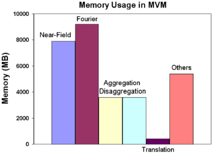
In addition to the memory complexity of MLFMA’s major parts, the memory size of these parts should also be investi-gated. The memory usage during iterations of a problem with 540 million unknowns is given in Fig. 1.
Fig. 1. Amounts of memory required by the data structures used in the MVM part of MLFMA for a problem that contains 540 million unknowns.
Radiation/receiving patterns (shown as “Fourier” in Fig. 1) and near-field interactions allocate most of the memory space during MVMs, and they are calculated once to be used several times. These aspects make them suitable to be used out of core. In the setup part of the algorithm, near-field interactions and radiation/receiving patterns are calculated in blocks of arrays and stored out of core to be used in the iterative solution part. During the iterative solution, first the near-field MVM is handled and then the near-field array is used out of core in small array pieces. Second, the near-field interactions are calculated and then the radiation/receiving patterns are used out of core.
B. Benchmarks
To test the effectiveness of the out-of-core method, we consider a set of scattering problems involving conducting spheres and their MLFMA solutions with various numbers of unknowns. Both solid-state drives (SSDs) and ordinary hard-disk drives (HDDs) are used, and similar results are obtained. Data is saved out of core in binary form to reduce the I/O time. The duration and the allocated memory to perform an MVM is
recorded for each problem; the results are presented in Table II, where the first column presents the problem size in terms of the number of unknowns. The second and the third columns present the elapsed time to perform an MVM, without out-of-core and with out-of-out-of-core implementations, respectively. The fourth and the fifth columns present the allocated memory per-process to perform an MVM. The solutions are obtained using 64 processes.
As evident from Table II, when the out-of-core technique is implemented, CPU time increases as the allocated memory decreases. This is due to slow I/O speed of the storage unit. In other words, taking advantage of the memory-saving out-of-core method extends the CPU time of the solution. Even so, the out-of-core method enables solving large-scale problems with limited memory.
TABLE II
TIMINGS ANDMEMORYSAVINGS OFOUT-OF-COREIMPLEMENTATION Unknowns MVM Time (seconds) MVM Memory (MB)
(Millions) MLFMA Out-of-Core MLFMA Out-of-Core
0.8 2 3 80 19 1.5 4.3 6.3 146 38 3.3 7.8 12.1 308 64 23.4 73.8 151 2278 541 53.1 176 199 4243 963 93.6 357 482 7224 2245
IV. PARALLELIZINGDATASTRUCTURES
Parallelization of MLFMA enables solving large-scale elec-tromagnetics problems that cannot be solved using the se-quential MLFMA. The setup and iterative-solution parts of MLFMA were already parallelized efficiently [4-6]. Paralleliz-ing the pre-processParalleliz-ing step was omitted because of its low memory usage compared to the memory of the setup and iterative-solution parts.
Sequential pre-processing is performed by a single process, while other processes remain idle. In systems with low per-node memory, pre-processing becomes a memory bottleneck because of the limited memory of the node on which the processing runs. To overcome this memory bottleneck, the pre-processing step is parallelized by means of distributing the input geometry data among the processes.
To parallelize the pre-processing step, we partition the components of the input geometry, such as nodes, triangles and edges, among the processors in a load-balanced manner. Assume that there is a one-to-one correspondence among the processors and processes, so that these two terms can be used interchangeably. In the pre-processing step, every processor needs the information of the whole geometry, but since the geometry data is partitioned, each processor only has a portion of it. To resolve this issue, data portions are transferred among the processes for any processor to reach any portion of data. To be more precise, each processor does its calculation on its initial portion of data and translates the data to another processor. Then the processors perform the same procedure on their temporary data. After p iterations, each process will have
accessed every other process’ portion of data and will retrieve its own initial data, where p is the number of processes.
Figure 2 illustrates the communication scheme of four processors. Here, pi denotes the processes and di denotes the
portions of distributed data, where 0 ≤ i < p and i is the process ID. In every iteration, processes access their required information from their temporary data, then send the data to their consequent process in terms of the process ID, i.e., at the end of every iteration, p1 gives its data to p2, p2gives its
data to p3, and so on. In that way, data is translated among
the processes in a cyclic manner, and every process accesses the information of the whole geometry.
Fig. 2. Cyclic communications among the processors.
V. NUMERICALRESULTS
To demonstrate the memory reduction of MLFMA, we consider a set of solutions for a conducting sphere, discretized with different numbers of unknowns. The sphere has a radius of 0.3 m, and it is meshed using equilateral triangles. The average mesh size is chosen to be 0.1λ.
We use a 16-node cluster with 2 TB of total memory. We record the allocated memory spaces at certain check-points to observe the memory consumptions of MLFMA and reduced-memory MLFMA (RM-MLFMA). The memory checkpoints are chosen such a way that the recorded memory is updated whenever a memory allocation or deallocation is made. Figures 3 and 4 show the recorded memory usage of the programs: the pre-processing step is performed between memory checkpoints 1-31, the setup part is performed be-tween memory checkpoints 31-43, and the MVMs start after memory checkpoint 43. We consider only the first 60 memory checkpoints because memory usage does not increase after the MVMs have started.
Figure 3 illustrates the memory consumptions of MLFMA and RM-MLFMA for various problems. The solutions of prob-lems with 135 million unknowns and 375 million unknowns are achieved using MLFMA, whereas the solution of the
Fig. 3. Memory consumption of MLFMA and RM-MLFMA per process.
Fig. 4. Total memory requirements of RM-MLFMA solutions for various problems using 64 processes.
problem with 684 million unknowns is achieved using RM-MLFMA. The programs are run on 128 processes. As Fig. 3 shows, in MLFMA, the peak memory grows rapidly when the problem size increases from 135 million unknowns to 375 million unknowns. On the other hand, with RM-MLFMA, we can solve a problem with 684 million unknowns by allocating almost the same amount of peak memory as to the problem with 375 million unknowns. The memory savings of RM-MLFMA highlights the importance of the proposed methods in terms of solving large-scale problems with limited computer resources.
To observe the memory scaling of large-scale scattering problems, we fill the arrays of RM-MLFMA without perform-ing any calculations, usperform-ing 64 processes. The results given in Fig. 4 show that we can handle a problem with 1, 233, 460, 224 unknowns within a total memory space of 1.83 TB.
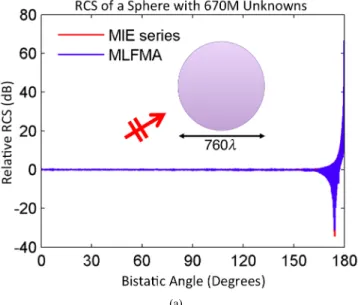
As an example, we present the results of an extremely large scattering problem solved with RM-MLFMA.The sample
(a)
(b)
Fig. 5. RCS of a sphere with 670 million unknowns. (a) 0◦< θ < 180◦ and (b) 178◦< θ < 180◦.
problem involved a conducting sphere with a radius of 380λ and 670, 138, 368 unknowns. The iterative solver converged in 30 iterations to satisfy a 1% residual error. Using 128 processes, the CPU time of the program was 40 hours and the total peak memory was 955 GB. The radar cross section (RCS) of the solution is presented in Fig. 5. Computational results obtained with RM-MLFMA agree well with the analytical Mie-series solutions.
VI. CONCLUSIONS
Memory reduction is achieved for MLFMA by using an out-of-core storage strategy and by parallelizing the pre-processing data structures. In order to eliminate some of the most significant memory bottlenecks, the out-of-core method is implemented on data structures during MVMs, and par-allelization is implemented on the largest data structures
used during the pre-processing steps. Numerical results are presented to demonstrate the memory-reduction ability of these methods. With the reduced-memory MLFMA, large-scale electromagnetic scattering problems are solved involving as many as 670 million unknowns with less than 1 TB memory. We also present numerical evidence to indicate that 1.3 billion unknowns can be solved with 2 TB memory.
ACKNOWLEDGMENTS
This work was supported by the Scientific and Technical Research Council of Turkey (TUBITAK) under Research Grants 110E268 and 111E203, by Schlumberger-Doll Re-search (SDR), and by contracts from ASELSAN, Turkish Aerospace Industries (TAI), and the Undersecretariat for De-fense Industries (SSM). Computer time was provided in part by a generous allocation from Intel Corporation. The authors would like to thank Jamie Wilcox of Intel Corporation for providing invaluable expertise to facilitate the benchmarking experiments on parallel computers.
REFERENCES
[1] M. Yuan, T. K. Sarkar, and B. M. Kolundzija, “Solution of large complex problems in computational electromagnetics using higher-order basis in MoM with out-of-core solvers,” IEEE Antennas Propagat. Mag., vol. 48, no. 2, pp. 55–62, 2006.
[2] X. W. Zhao, Y. Zhang, H. W. Zhang, D. G. Donoro, S. W. Ting, T. K. Sarkar, and C. H. Liang, “Parallel MoM-PO method with out-of-core technique for analysis of complex arrays on electrically large platforms,” Prog. Electromagn. Res., vol. 108, pp. 1–21, 2010.
[3] J. M. Song and W. C. Chew, “Multilevel fast-multipole algorithm for solving combined field integral equations of electromagnetic scattering,” Microwave Opt. Tech. Lett., vol. 10, no. 1, pp. 14–19, 1995.
[4] ¨O. Erg¨ul and L. G¨urel, “Efficient parallelization of the multilevel fast multipole algorithm for the solution of large-scale scattering problems,” IEEE Trans. Antennas Propag., vol. 56, no. 8, pp. 2335–2345, 2008. [5] ¨O. Erg¨ul and L. G¨urel, “A hierarchical partitioning strategy for an
efficient parallelization of the multilevel fast multipole algorithm,” IEEE Trans. Antennas Propag., vol. 57, no. 6, pp. 1740–1750, 2009. [6] L. G¨urel and ¨O. Erg¨ul, “Hierarchical parallelization of the multilevel
fast multipole algorithm (MLFMA),” Proc. IEEE, vol. 101, no. 2, pp. 332–341, Feb. 2013.