Variations in normal color vision. IV. Binary hues
and hue scaling
Gokhan Malkoc*
Department of Psychology, University of Nevada, Reno, Reno Nevada 89557 Paul Kay
International Computer Science Institute, Berkeley, California 94704, and University of California, Berkeley, California 94720
Michael A. Webster
Department of Psychology, University of Nevada, Reno, Reno Nevada 89557 Received February 22, 2005; accepted May 6, 2005
We used hue cancellation and focal naming to compare individual differences in stimuli selected for unique hues (e.g., pure blue or green) and binary hues (e.g., blue-green). Standard models assume that binary hues depend on the component responses of red–green and blue–yellow processes. However, variance was compa-rable for unique and binary hues, and settings across categories showed little correlation. Thus, the choices for the binary mixtures are poorly predicted by the unique hue settings. Hue scaling was used to compare indi-vidual differences both within and between categories. Ratings for distant stimuli were again independent, while neighboring stimuli covaried and revealed clusters near the poles of the LvsM and SvsLM cardinal axes. While individual differences were large, mean focal choices for red, blue-green, yellow-green, and (to a lesser extent) purple fall near the cardinal axes, such that the cardinal axes roughly delineate the boundaries for blue vs. green and yellow vs. green categories. This suggests a weak tie between the cone-opponent axes and the structure of color appearance. © 2005 Optical Society of America
OCIS codes: 330.1690, 330.1720, 330.5020, 330.5510.
1. INTRODUCTION
Conventional models of color appearance hold that the perception of color is organized according to a small num-ber of privileged axes.1–5 In Hering’s theory of color op-ponency, one of these axes represents variations in light-ness or darklight-ness while the other two encode the opposing dimensions of red vs. green and blue vs. yellow.6By this account, the unique hues (colors that appear pure red, green, blue, or yellow) are special because they reflect the undiluted response of a single opponent process. All other hues are binary hues because they instead reflect mix-tures of red or green with blue or yellow. For example, or-ange is composed of red and yellow, while purple is a blend of red and blue.7,8Thus binary hues have a status subordinate to the unique hues because they have no rep-resentation in the model other than in terms of the con-tributions of the underlying unique hues. The stimuli cor-responding to unique hues can be found by varying a spectral stimulus until it appears pure (e.g., to find the point at which a red stimulus appears untinged by blue or yellow).9–12More generally, the red–green or blue–yellow responses to any stimulus can be measured by physically nulling the hue sensation (e.g., by adding a “green” light to the stimulus until any redness in the stimulus is canceled)13or by scaling the component sensations (e.g., by judging the relative amounts of red and yellow that make up an orange stimulus).14–17
Another approach to studying color appearance has
been to test for consensus in color naming across observ-ers. Berlin and Kay18found that languages have only a small number of basic color terms, in the sense that the terms are monolexemic, used consistently by different speakers, and refer to color independent of particular ob-jects. They also showed that the basic terms in different languages tend to be focused on very similar regions of color space, and that while languages vary in the number of basic terms, these follow a highly constrained order. For example, as refined in later work, a language with two terms is likely to have one encompassing white, red, yellow, and other “warm” colors with the other encom-passing black, green, blue, and other “cool” colors. More recently, this broad pattern has been verified by analyses of color naming from the 110 unwritten languages sampled by the World Color Survey.19–22The centroids of the stimuli labeled by basic color terms in these lan-guages cluster strongly around similar points in color space, showing that respondents view the spectrum in very similar ways regardless of the varying number of categories into which their lexicons partition it. While counterexamples have been noted (e.g., Ref. 23), the simi-lar clustering across languages suggests that the special and shared status of basic color terms may reflect special and shared properties of the human visual system or of the visual environment.
Like the unique hues, the evidence for basic color terms implies that some stimuli have a privileged status in color 1084-7529/05/102154-15/$15.00 © 2005 Optical Society of America
appearance. Indeed, when given comparable stimulus sets, English-speaking observers select the same stimuli for unique hue settings as they do when choosing the best example or focal stimulus for red, green, blue, or yellow.24,25 However, basic color terms are not restricted to the set of primaries given by the three opponent axes. For example, English has 11 basic terms, which include the Hering primaries (white, black, red, green, blue, yel-low, and a neutral gray) but also secondary colors (orange, purple, pink, and brown).18Thus, by the criterion of con-sensus color naming, orange in English has a status simi-lar to that of red or yellow and may have a status superior to that of a comparable mixture category such as yellow-green, for which there is not a basic term. Moreover, the stimuli labeled by different basic color terms do not sup-port the independence of the luminance and chromatic di-mensions assumed by many color-opponent models. For example, green and blue terms apply to stimuli over a wide range of lightness levels, while red is restricted to low values and yellow is used only for stimuli with a high lightness.18,21,26 Thus the specific structure of color ap-pearance implied by the standard three-channel model of color opponency and by basic color terms differ, and this circumstance has led to suggestions that there may be an explicit neural process corresponding to each of the 11 ba-sic categories.26
In this study we examined the structure of color ap-pearance by observing individual differences in color naming. Subjects with normal color vision have been pre-viously shown to vary widely in the stimuli they select for the unique hues10,27–31and in the focal stimuli they select for basic color terms.18,21,22,31Thus a yellow that appears distinctly reddish to one observer might appear strongly greenish to another. In previous studies of these varia-tions, we found that the stimuli observers choose for dif-ferent unique hues are largely uncorrelated.10 For ex-ample, a subject whose unique yellow is more reddish than average is not more likely to choose a unique blue that is more reddish (or more greenish) than average. The independence of the unique hues is surprising given that many factors that affect visual sensitivity (such as differ-ences in screening pigments or in the relative numbers of different cone types) should influence different hues in similar ways and thus predict strong correlations
be-tween them.10However, a number of studies have shown
that the unique hue loci are not in fact clearly tied to mea-sures of visual sensitivity29,32–35and may instead reflect learning or adaptation to specific properties of the color environment.34,36–39 By either account, our results sug-gest that the variations in the axes for the red–green and blue–yellow dimensions of color appearance—or between the two poles of the same opponent axis—are controlled by independent factors.
In the present study our aim was to look more closely at the patterns of variation in color naming by sampling color space more finely. In particular, we were interested in the range in color space over which hue choices are cor-related and whether different patterns emerge for the unique hues and intermediate hues. For example, even if the selections for red and yellow are uncorrelated, to the extent that orange reflects the combined “responses” of red and yellow, the loci for orange might be expected to
covary with the loci of the underlying primaries. Alterna-tively, if focal orange is fine tuned by its own physiological or environmental constraints, then it might instead float freely between red and yellow. In turn, hues like orange and purple for which English has basic color terms might vary in different ways than blue-green or yellow-green, which may instead correspond more to the boundaries be-tween categories. Comparing individual differences in the unique and binary hues might thus provide clues about the nature and number of the processes calibrating color appearance. A further goal of our study was to extend measures of individual differences in color appearance to include the dimensions of saturation and lightness and thus to characterize the patterns of variations more fully within the volume of color space. Our results show that the range of individual differences in color naming is similar for unique and binary hues and that there are again only weak correlations between the color categories from neighboring regions of color space. Thus, by these criteria, the unique hues do not emerge as special and do not alone fully anchor the structure of color appearance for an individual.
2. METHODS
Stimuli were presented on a Sony 20se monitor controlled by a Cambridge Research Systems VSG graphics card. The monitor was calibrated with a PR650 Spectracolorim-eter, and gun luminances were linearized through look-up tables. The test colors were presented on a uniform 6 deg!8 deg background provided by the monitor screen.
The background had a mean luminance of 30 cd/m2and a
mean chromaticity equivalent to Illuminant C (CIE 1931 x=0.31, y=0.316). (Note this differs from conventional studies of the unique hues, which have instead typically used narrowband stimuli presented on a dark back-ground, but it has the advantage that we could explore the foci for moderately saturated lights under steady ad-aptation. To the extent that observers are adapted to the background, the results are unlikely to depend on the choice of the specific chromaticity chosen for the neutral background.16,40,41)
Color and luminance were specified in terms of a scaled
version of Derrington, Krauskopf, and Lennie42 color
space, in which the origin corresponded to the background color and contrast varied as a vector defined by the lumi-nance, LvsM and SvsLM cardinal axes. Units in the space were related to the r, b chromaticity coordinates in
MacLeod–Boynton43 space and to Michelson luminance
contrast!Lc" by
LvsM contrast =!rmb− 0.6568"*2754, SvsLM contrast =!bmb− 0.01825"*4099,
LUM = 3*L c.
We used three sets of stimuli and procedures to measure individual differences in color judgments.
A. Unique and Binary Hue Settings
In the first case, subjects made both unique hue settings (for red, green, blue, or yellow) and binary hue settings (for orange, purple, yellow-green, or blue-green). Stimuli were moderately saturated isoluminant pulses, presented at the full contrast for 1 s and ramped on and off with a Gaussian envelope (with a standard deviation of 250 ms). The stimuli all had the same maximum contrast of 80 in the space and thus varied only in hue angle within the LvsM and SvsLM plane, with isoluminance defined pho-tometrically. The hues were presented in a central 2-deg field demarcated from the 6!8 deg background by a nar-row black outline. Between stimuli the field remained at the same gray as the background.
For each setting, subjects first adapted to the gray background for 1 min. Hue loci were then estimated with a 2AFC staircase procedure. On each trial, the observer responded whether the target hue was biased toward one of the target’s neighboring hues or the other. For example, for unique red, they responded whether the color ap-peared either too purple or too orange, while for purple they responded too blue or too red, etc. Successive hues were then varied using two randomly interleaved stair-cases, with the hue angle estimated from the mean of the final six of ten reversals from both staircases. During a 1-h session the eight hues were tested two times each in random order and were retested in a second session for each subject approximately one week later. Observers were 73 students at the University of Nevada, Reno (UNR). All subjects were screened for normal color vision by the Neitz Color Test44and the Ishihara pseudoisochro-matic plates and were naïve with regard to the specific aims of the study.
B. Individual Differences in Hue, Lightness, and Contrast
In the second experiment, stimuli were varied not only in hue but also in lightness and saturation, in order to com-pare the variations for each color in terms of the three principal attributes of color appearance. Because this re-quired varying the stimuli along three dimensions in-stead of one, we used a different procedure in which sub-jects were shown a palette of colors at a fixed contrast, and then selected the best example of a given color term from this palette. This procedure was thus more similar to the types of procedures used in cross-linguistic studies of color naming. In the present case, the palette was com-posed of a 9!9 array of stimuli that varied in hue across columns and in lightness across rows, with the lightness and hue steps equated within the scaled space defined above. Each circular patch subtended 1.15 deg with 1.3 deg between the patch centers. The background in this case subtended 15!20 deg. The term to be selected for was written in the upper left corner of the background. Subjects were first shown a broad range of colors span-ning a hue angle of 112 deg centered at random points in color space around the nominal focal stimulus, and they selected the best patch for the term indicated by using a keypad to move a thin black ring over the array to high-light their choice. The next five trials then zoomed in at random points around the selected chip and showed a much finer color array spanning 45 deg in color angle that
was centered at random points around their color selec-tion. During a given run all stimulus arrays had a fixed contrast, with the eight color terms and five repetitions presented in random order. Color terms again included the four unique hues and the four binary terms. Contrast across runs varied in random order in steps of 20 units, from 20 up to the maximum contrast available for a given region of the space. A separate new sample of 53 UNR stu-dents participated in this experiment. As before, these subjects were all screened for normal color vision and re-peated the settings in two daily sessions.
C. Hue Scaling
To provide a still finer sampling of color space, in the final condition we used a hue scaling task to rate the color ap-pearance of 24 isoluminant stimuli falling at intervals of 15 deg along a circle spanning the LvsM and SvsLM plane. These stimuli all had a fixed contrast of 80 and were again shown in a square 2-deg field, pulsed for 1 s as in the unique and binary hue settings described in the first condition above. The scaling procedure followed the procedure used by De Valois and colleagues.16 For each stimulus, subjects rated the hue by pressing separate but-tons to indicate the relative amounts of red, green, blue, or yellow. For example, the response to a reddish orange might be three red presses and two yellow. Subjects were instructed to use at least five presses to score the color but were allowed to use more if they wanted to use finer scal-ing (e.g., seven red and one yellow for a red that appeared only slightly tinged with yellow). Each angle was pre-sented five times in random order, and subjects repeated the settings on a second day. On a separate run during the session the hues were again shown, and subjects se-lected a color label for the hue by choosing from the four unique and four binary terms displayed at the bottom of the screen. A separate sample of 59 additional color-normal students took part in these settings.
3. RESULTS
A. Unique and Binary Hue Settings
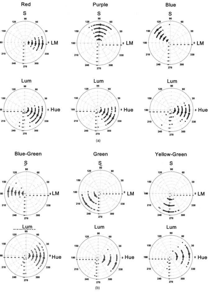
Figure 1 plots the mean hue angles chosen by individual subjects for each of the color terms tested. The average angles across subjects and their range are given in Table 1. As in previous studies,28the range of variation in the hue settings is pronounced, to the extent that the range of focal choices for neighboring color terms often overlap. Thus some subjects chose as their best example of orange a stimulus that other subjects selected as the best ex-ample of red, while others selected for orange a stimulus that some individuals chose for yellow. In fact, there was only one narrow region of the color circle, between red and purple, that did not receive choices for any of the eight terms.
Surprisingly, the degree of consensus among observers did not clearly distinguish unique from binary hues, nor basic terms from nonbasic terms. For example, both blue and green spanned a relatively large range of hue angles, while the narrowest range was for blue-green. Thus there was much greater agreement between subjects about the border separating the blue and green categories than about the focal stimulus for either category. Of course,
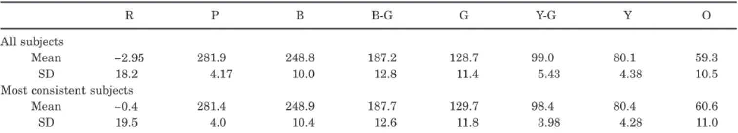
this comparison depends on the choice of space. The cone-opponent space explicitly captures how the hues vary in terms of the dimensions underlying early postreceptoral color coding but makes little assumption about the sa-lience of hue differences along different chromatic angles and thus may fail to reveal the perceptual magnitude of the spread for each hue. To explore this, Table 2 gives the mean and standard deviation of the hue angles converted
to the CIE u
!
v!
space, which is designed to roughlyequate the perceptual distances between different regions of color space. Within this space the range for red and blue-green are greatly expanded, while yellow and purple are contracted. Yet it is still the case that as a group the unique hues do not differ from the binary hues in the de-gree of consensus.
Within the cone-opponent space of Fig. 1 the blue-green settings are not only narrow but are also notable for fall-ing close to the +M/−L pole of the LvsM axis (especially since the empirically defined axis may be rotated slightly clockwise relative to the nominal axis that we used based on the standard observer).45Red is well known to be the only unique hue that lies near one of the cardinal axes.10,16,46,47 However, the fact that blue-green settings cluster tightly around the opposite pole of the LvsM axis indicates that the blue and green categories (if not the unique points) may also be more closely associated with the cardinal axes than normally supposed. In particular, whether a stimulus appears more green or more blue (and whether a red appeared too blue or too yellow) depends roughly on whether it results in more or less S-cone exci-tation relative to the background. However, as with the unique red settings, this is only a very rough correspon-dence, for the range of individual differences in the color choices far exceeds the plausible range of variation in the stimulus angles isolating the LvsM axes for different observers.45,48It is also notable that the average settings for yellow-green fall close to one of the poles of the SvsLM axis (and that purple skirts the opposite pole, though in this case the average differed more clearly from the S axis). Thus again, while focal yellow or green lies at inter-mediate angles in terms of the cardinal axes, the partition defining whether a color is too yellow or too green falls roughly at the SvsLM axis and thus depends on whether the hue has a larger or smaller L/M ratio than the back-ground. (Again this must at best be a very rough corre-spondence, yet the SvsLM axis is more strongly affected than the LvsM axis by factors such as variations in macu-lar pigment density, and thus the range of potential varia-tion in the SvsLM cardinal axis is much larger.45,48)
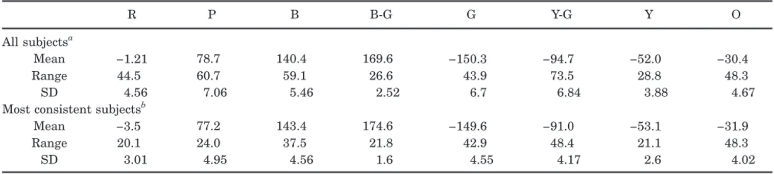
Table 3 shows the correlations between the settings for the different color terms. Previously we found that there is little correlation either among unique hue choices10or among different focal judgments for the unique hue terms.22The present results confirm this and, moreover, Table 1. Mean Hue Angles for Unique and Binary Hues in the Scaled LvsM and SvsLM Space and the
Range and Standard Deviation (SD) across Observers
R P B B-G G Y-G Y O
All subjectsa
Mean −1.21 78.7 140.4 169.6 −150.3 −94.7 −52.0 −30.4
Range 44.5 60.7 59.1 26.6 43.9 73.5 28.8 48.3
SD 4.56 7.06 5.46 2.52 6.7 6.84 3.88 4.67
Most consistent subjectsb
Mean −3.5 77.2 143.4 174.6 −149.6 −91.0 −53.1 −31.9
Range 20.1 24.0 37.5 21.8 42.9 48.4 21.1 48.3
SD 3.01 4.95 4.56 1.6 4.55 4.17 2.6 4.02
aResults for all 73 subjects.
bResults for the 21 subjects who set the hues most consistently.
Fig. 1. Mean hue angles selected by individual observers for the eight different color terms. (a) all observers, (b) settings for the subset of observers who selected the hues most consistently.
show that the settings for both unique and binary hues are also largely uncorrelated. The independence of the unique hues is surprising in two regards. First, many models of color appearance assume that the opponent hues (e.g., blue and yellow) are shaped by common factors (e.g., the equilibrium axis for the red–green dimension). Yet these factors do not appear to strongly constrain how individuals vary within each category. Second, as we noted at the outset, most conventional models of color ap-pearance assume that the binary hues are represented only in terms of the underlying unique hues. Yet the indi-vidual choices for the binary categories cannot be pre-dicted from the choices for either component unique hue. The lack of consistent correlations between the differ-ent hues across subjects could occur if individual subjects were inconsistent in their hue settings. In fact, the diag-onal cells in the matrix of Table 3 show the correlation be-tween the settings for the same color across the two ses-sions, and these are low for some of the terms. (Note that this does not directly imply that subjects were unreliable in their settings but only that they were inconsistent rela-tive to the range of variation across the group.) To test whether intraobserver variation was masking a depen-dence between the different hues, we reanalyzed the set-tings for the subset of observers who chose the focal stimuli with the highest reliability (as in our previous
study10). Subjects were chosen by excluding any observer whose range of four settings (two from each daily session) exceeded the mean range on any color by more than 1.5 standard deviations. This left a pool of 21 observers whose results are shown in Fig. 1(b) and in the lower halves of Tables 1 and 3. For this subset, the consistency of repeated settings was much higher, while the variance between observers was roughly halved. However, indi-vidual differences remained substantial. Moreover, the correlations among different hues remained weak. Thus the independence regarding the different hue settings is unlikely to be an artifact of noise in the observers’ set-tings.
We also asked whether the weak dependence between unique and binary hues occurred because we correlated only pairs of colors. If blue and green vary independently, then if blue-green represented a “halfway point” between them, it might be tied more closely to the average of an observer’s blue and green loci rather than to the setting for either color alone. We therefore compared the correla-tions between each hue and the mean of its two neighbors (Table 4). This comparison showed a consistent relation-ship with the bounding neighbors for yellow and for or-ange but still weak dependence on the bounding neigh-bors for the other colors and no clear tendency for unique and binary hues to behave differently. This again sug-Table 2. Mean and Standard Deviation (SD) of the Hue Angles within the u
!
v!
Uniform Color SpaceR P B B-G G Y-G Y O
All subjects
Mean −2.95 281.9 248.8 187.2 128.7 99.0 80.1 59.3
SD 18.2 4.17 10.0 12.8 11.4 5.43 4.38 10.5
Most consistent subjects
Mean −0.4 281.4 248.9 187.7 129.7 98.4 80.4 60.6
SD 19.5 4.0 10.4 12.6 11.8 3.98 4.28 11.0
Table 3. Correlations between Hue Angles Chosen for Different Color Termsa
R P B B-G G Y-G Y O All subjects R 0.57* 0.23!* −0.05 0.0 −0.29!* −0.06 −0.07 0.01 P 0.39* 0.31!* −0.04 −0.09 −0.07 −0.16 −0.10 B 0.67* 0.02 0.02 0.02 −0.29!* −0.17 B-G 0.60* 0.19 0.05 −0.14 −0.12 G 0.61* 0.12 −0.23!* −0.12 Y-G 0.57* 0.19 0.04 Y 0.31* 0.45!* O 0.66*
Most consistent subjects
R 0.61* 0.27 0.06 0.13 0.19 0.09 −0.20 0.23 P 0.40* 0.12 0.22 0.16 0.12 −0.28 −0.13 B 0.83* 0.34 0.11 0.09 −0.32 −0.36 B-G 0.85* 0.25 0.13 −0.40 −0.06 G 0.84* −0.18 −0.47!* −0.33 Y-G 0.83* 0.18 0.05 Y 0.77* 0.56!* O 0.82*
gests that there is little joint constraint on the individual foci for unique and binary hues.
B. Effects of Lightness and Contrast
In the next set of experiments we asked how the focal color settings depended on the lightness and contrast of the stimuli. As noted in Section 2, this required sampling a much wider range of colors, and we therefore changed the procedure so that subjects picked the focal stimuli from a palette. The selections for individual observers are shown in Fig. 2. For each of the eight colors, the top panel shows the chosen hue angles within the LvsM and SvsLM chromatic plane (similar to Fig. 1), and the bottom panel plots the elevation out of the isoluminant plane. Succes-sive radii show the settings at contrasts ranging from 20 to 100 units. For orange, the monitor gamut limited the maximum contrast at higher lightnesses to 80, and for yellow, green, and yellow-green, the maximum was 60. Fewer settings are therefore shown for these colors (and are shown with a different scaling for the radii).
Relative to the settings in the preceding cancellation task, mean hue angles in the present task tended to be biased away from the LvsM and toward the SvsLM axis, perhaps reflecting weaker sensitivity to SvsLM contrast in the palette stimulus. Note also that for these settings the stimuli varied along spheres of fixed radius within the cone-opponent space. Thus increasing or decreasing the lightness outside the isoluminant plane required a trade-off between luminance contrast and chromatic contrast and in this sense provided a measure of the relative im-portance of hue and lightness for the focal choices. That is, stimuli with a high lightness could be chosen only by sacrificing chromatic saturation. Nevertheless, for certain color terms the focal choices had a strong lightness com-ponent. For example, most subjects chose stimuli for red and purple that were darker than the background, while for yellow the focal choices had a higher lightness. This confirms previous studies in showing that lightness level is an important dimension of some focal colors and of yel-low in particular.26Consistent with this, yellow also had the lowest variance in the lightness settings, while for all other colors the standard deviation of the lightness angles exceeded those for the corresponding hue angles. This
could indicate that lightness is less important to the judg-ment. However, an alternative is that subjects vary more in their preferred lightness values. In fact, we have re-cently found that the focal choices for different languages in the World Color Survey differ more in their lightness settings than in their hue settings (relative to the respec-tive within-language variations),22 and thus it is likely that the variations in lightness levels do partly reflect ac-tual variations in subject’s preferences.
This is further suggested by the relationships among different lightness settings. Table 5 shows the correlation matrix among the eight color terms. Values below the di-agonal give the correlations between the hue angles and are consistent with the preceding experiment in showing that the variations between hues are largely independent (though notably the strongest correlation is again be-tween orange and yellow). The cells above the diagonal give the corresponding values for the lightness settings. The correlations are again weak overall, yet they are clearly stronger than for the hue settings, and in all cases the significant values are positive. This suggests that, un-like the hue settings, the lightness settings for individual observers revealed a general tendency to choose lighter or darker samples for their focal stimuli.
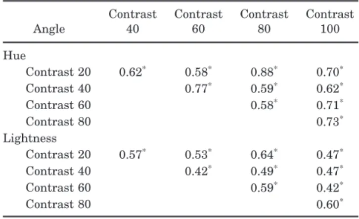
Unlike both hue and lightness, the correlations in the foci across different contrast levels were strong. Table 6 illustrates these for the red settings. (The pattern for the other colors was similar.) Because different contrasts and color terms were randomly intermixed during testing, such results suggest that in this task subjects were rela-tively consistent at selecting the same color-luminance angle in their settings, regardless of the contrast of the stimulus. In turn, this finding reinforces the conclusion that the choices for different terms are largely indepen-dent and that this independence reflects actual differ-ences between observers rather than variance within the observers’ settings. Moreover, it suggests that the differ-ences between observers are largely captured by the color-luminance angles of their stimuli.
C. Hue Scaling
The preceding results showed that the variations in focal colors across neighboring color categories are largely in-dependent. That is, the color a subject selects for red does not predict his or her selection for orange. In the final ex-periment we explored the pattern of variation not only across but also within color categories—for different shades of red or orange—by measuring individual differ-ences in a hue scaling task. As noted in Section 2, in this case the stimuli were 24 hues spanning the LvsM and SvsLM plane at intervals of 15 deg. Subjects judged the hue by rating the relative amount of red, green, blue, or yellow. These ratings were then converted into a hue angle within a perceptual opponent space defined by the
pure red–green !0–180 deg" and blue–yellow
!90–270 deg" axes. For example, a stimulus that was rated three parts blue and two parts red would have an angle of tan−1!3/2"=56.3 deg within the perceptual red vs. green and blue vs. yellow space. Figure 3(a) shows the relationship between the stimulus angle in the cone-opponent space and the average perceptual hue angle for the observers. On separate trials each observer also la-Table 4. Correlation between the Angles Chosen
for Each Term and the Mean of the Angles for the Two Bounding Termsa
Hue SubjectsAll ConsistentSubjects Primary
Red vs. orange/purple 0.21 0.36
Green vs. blue-green/yellow green 0.18 −0.05 Blue vs. blue-green/purple 0.30* 0.27 Yellow vs. orange/yellow-green 0.39* 0.53* Binary Purple vs. blue/red 0.40* 0.22 Blue-green vs. blue/green 0.15 0.38 Yellow-green vs. yellow/green 0.22 −0.11 Orange vs. yellow/red 0.31* 0.65* a *p"0.05.
Fig. 2. Individual settings for the hue and lightness of each of the eight color terms. For each term, the top panel plots the selected hue angle projected onto the isoluminant plane (i.e., independent of the subject’s lightness setting), while the bottom panel shows the eleva-tion out of the isoluminant plane (i.e., independent of the subject’s selected hue angle). Settings for stimuli of increasing contrast are plotted along circles of increasing radii. (Continues on next page.)
beled the stimulus with one of the eight color terms. The distribution of these labels is shown in Fig. 4.
Not surprisingly, the ratings in the hue scaling task are qualitatively consistent with how stimuli were selected in the focal color task. It is again interesting to ask how these ratings are related to the cone-opponent axes used to define the stimuli. In Fig. 3(a) the arrows mark the in-tersection of each pole of the cardinal axes with the nomi-nal perceptual axis (the four unique hues or the equal bi-nary mixtures of these hues) that was nearest to the scaled hue. As before, the +L axis falls close to unique red, while the remaining cone-opponent axes lie close to the binary axes. (A similar pattern can be seen in the results of De Valois et al.49) That is, the −L pole was, on average, rated as nearly an equal mixture of blue and green, while the −S pole was a balanced mixture of green and yellow. Thus, like the focal choices, these results point to a rela-tionship between the structure of cone-opponent space
and the structure of color appearance (a relationship that is again very loose because of the large individual differ-ences). Three of the cone-opponent directions therefore represent boundaries between the unique hue axes (e.g., whether a stimulus is more green or more blue), while the fourth is “unique” in that it is aligned with the red pri-mary.
As with the focal color settings, subjects also varied widely in the hue scaling judgments. For the settings con-verted to angles in the RG–BY space, standard deviations for the individual stimuli ranged from 6 to 22 deg!mean =14 deg". We asked whether the variation in the range for different stimuli might be predicted from the rate at which perceived color varies in different regions of color space. As Fig. 3(a) shows, perceived color as determined by the scaling task changes rapidly for stimuli moving from yellow to red, changing more slowly for transitions from red to purple. If individual differences in the ratings Table 5. Correlations between Hue Angles (below Diagonal) and Lightness Levels (above Diagonal) for
Different Color Terms Lightness R P B B-G G Y-G Y O R 0.02 0.11 0.12 0.21 −0.09 −0.06 0.09 P 0.15 0.30!* 0.34!* 0.17 0.08 −0.06 0.30!* B −0.03 0.01 0.56!* 0.29!* 0.20 0.13 0.28!* B-G 0.11 −0.14 0.23 0.34!* 0.10 0.10 0.36!* G −0.12 −0.24 −0.02 0.14 0.16 0.09 0.49!* Y-G 0.07 −0.08 0.08 −0.02 0.26 0.21 0.29!* Y −0.06 0.10 0.14 −0.16 −0.01 0.40!* 0.13 O −0.06 0.16 −0.03 −0.11 0.31!* 0.10 0.48!* Hue Fig. 2. (Continued).
reflected a fixed range of perceptual color difference, then this range should be related to the local slope of the hue
scaling function. These slopes were estimated from a poly-nomial fit to the mean hue scaling curve. Figure 3(b) com-pares the standard deviations in the ratings for each of the 24 stimuli (again with the ratings expressed as angles in the perceptual space) with the slope of the hue scaling function at each stimulus angle. There is little relation-ship between the two values, indicating that the variance in judgments probably does not depend on the salience of color differences in different regions of the space. This conclusion is also consistent with the analysis above showing that large differences in the ranges for different color terms remain when the stimuli are represented in a uniform color space such as u
!
v!
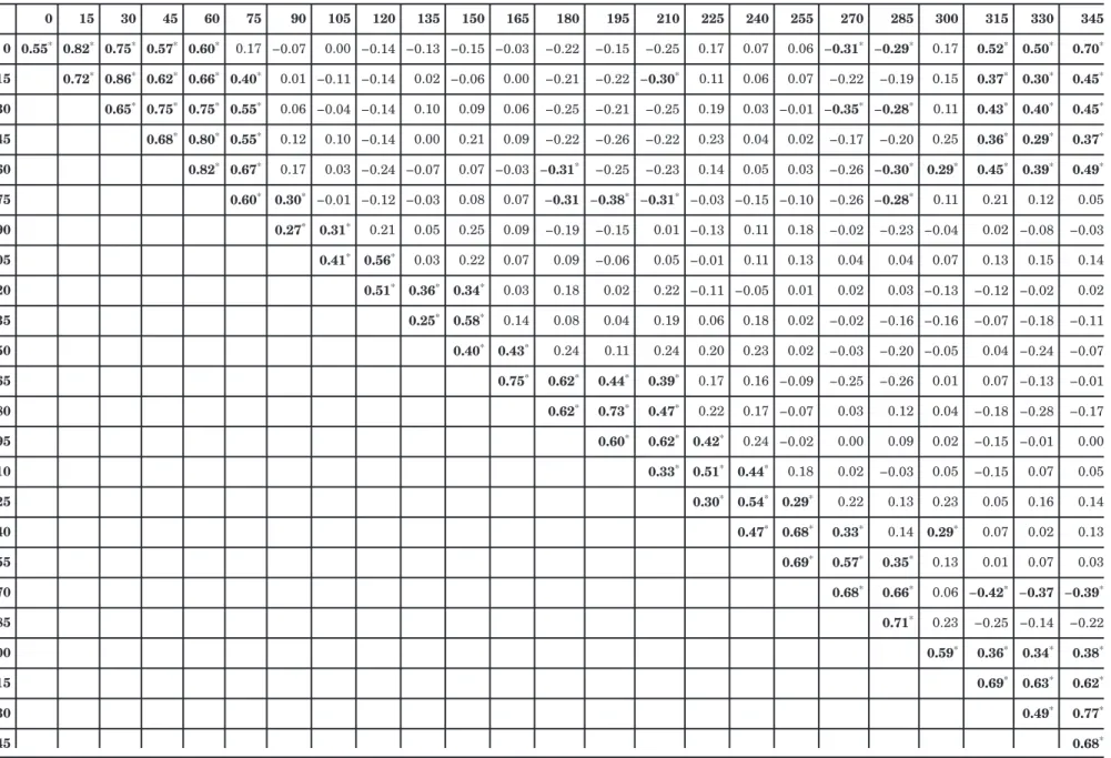
(Table 2).The correlations between the ratings for the different chromatic angles are shown in Table 7. It is clear that there tend to be strong correlations between nearby hue angles yet only weak relationships between more distant angles. Thus the variations in each hue again depend on relatively local factors. This is further seen in Table 8, which reproduces the values for the eight angles closest to the foci for the eight color terms. These were determined from the modal values in the distributions of color labels in Fig. 4. Like the results for focal choices, few of the color terms are significantly correlated (though once again or-ange emerges as a possible exception). In the case of the hue scaling, this is all the more surprising, because sub-jects could rate the stimuli only in terms of the four unique hues, yet the variations in scaling binary hues like purple did not depend on how subjects differed in scaling red or blue.
One possible basis for this pattern of local correlations is that each hue angle covaries consistently only with its nearby neighbors. However, there is instead a discrete clustering of the correlations. To visualize this, we calcu-lated for each stimulus the “center of mass” of its correla-tion coefficients, given by averaging the stimulus angles weighted by the coefficients. For these averages we used only coefficients that were significant and positive. The mean angles for each cluster are plotted as a function of the stimulus angle in Figs. 5(a) (for all subjects) and 5(b) (for the 30 most consistent subjects, whose repeated set-tings varied less than the median variance for all sub-jects). If the local correlations were centered at each stimulus angle, then these clusters would vary continu-ously and fall along the diagonal of the figure. Instead, there are clear steps, especially for the subset of consis-tent observers. One of these steps is centered on the +L pole of the LvsM axis and includes a wide span of stimu-lus angles ranging from −45 deg (orange) to 60 deg (red-dish purple). Over this span subjects differed consistently from each other in how they scaled the stimuli, while set-tings for neighboring stimuli just outside this cluster re-sulted in a new pattern of individual differences. Weaker clusters are also evident near 180 deg, the opposite pole of the LvsM axis, and at 270 deg, the +S pole of the SvsLM axis.
Recall again that in the hue scaling task the subjects were restricted to using four color terms (the perceived amounts of red, green, blue, and yellow). Thus it is pos-sible that the clustering simply reflects how subjects weighted the independent primaries. However, predic-Table 6. Correlations among the Hue Angles and
Lightness Levels Chosen for Focal Red across Different Contrast Levels
Angle Contrast40 Contrast60 Contrast80 Contrast100 Hue Contrast 20 0.62* 0.58* 0.88* 0.70* Contrast 40 0.77* 0.59* 0.62* Contrast 60 0.58* 0.71* Contrast 80 0.73* Lightness Contrast 20 0.57* 0.53* 0.64* 0.47* Contrast 40 0.42* 0.49* 0.47* Contrast 60 0.59* 0.42* Contrast 80 0.60*
Fig. 3. (a) Average hue scaling function. Points plot the judged angle in a red–green versus blue–yellow perceptual color space as a function of the stimulus angle in the LvsM and SvsLM plane. Arrows point to the perceived hues of stimuli lying along the cardinal axes and the closest unique or binary color term. (b) Relationship between individual differences in the hue scaling and the local slope of the average hue scaling function.
tions based on scaling or rotating the mean hue scaling response to red, green, blue, and yellow failed to fit the observed pattern of correlations or of factors derived from a factor analysis of the correlation matrix. Thus we are
uncertain of the basis for the clustering. Yet what-ever its basis, the individual differences in hue scaling do not ap-pear tied to differences in the relative strength or direc-tion of mechanisms tuned to the unique hue direcdirec-tions. Fig. 4. Distribution of color labels for the 24 stimuli used in the hue scaling task. Each panel shows the number of times subjects chose a given color term as the label for the stimulus. The eight panels show results for the four unique hue terms or the four binary terms.
Table 7. Correlations between the Rated Hues for Each of the 24 Stimuli in the Hue Scaling Task 0 15 30 45 60 75 90 105 120 135 150 165 180 195 210 225 240 255 270 285 300 315 330 345 0 0.55* 0.82* 0.75* 0.57* 0.60* 0.17 −0.07 0.00 −0.14 −0.13 −0.15 −0.03 −0.22 −0.15 −0.25 0.17 0.07 0.06 −0.31* −0.29* 0.17 0.52* 0.50* 0.70* 15 0.72* 0.86* 0.62* 0.66* 0.40* 0.01 −0.11 −0.14 0.02 −0.06 0.00 −0.21 −0.22 −0.30* 0.11 0.06 0.07 −0.22 −0.19 0.15 0.37* 0.30* 0.45* 30 0.65* 0.75* 0.75* 0.55* 0.06 −0.04 −0.14 0.10 0.09 0.06 −0.25 −0.21 −0.25 0.19 0.03 −0.01 −0.35* −0.28* 0.11 0.43* 0.40* 0.45* 45 0.68* 0.80* 0.55* 0.12 0.10 −0.14 0.00 0.21 0.09 −0.22 −0.26 −0.22 0.23 0.04 0.02 −0.17 −0.20 0.25 0.36* 0.29* 0.37* 60 0.82* 0.67* 0.17 0.03 −0.24 −0.07 0.07 −0.03 −0.31* −0.25 −0.23 0.14 0.05 0.03 −0.26 −0.30* 0.29* 0.45* 0.39* 0.49* 75 0.60* 0.30* −0.01 −0.12 −0.03 0.08 0.07 −0.31 −0.38* −0.31* −0.03 −0.15 −0.10 −0.26 −0.28* 0.11 0.21 0.12 0.05 90 0.27* 0.31* 0.21 0.05 0.25 0.09 −0.19 −0.15 0.01 −0.13 0.11 0.18 −0.02 −0.23 −0.04 0.02 −0.08 −0.03 105 0.41* 0.56* 0.03 0.22 0.07 0.09 −0.06 0.05 −0.01 0.11 0.13 0.04 0.04 0.07 0.13 0.15 0.14 120 0.51* 0.36* 0.34* 0.03 0.18 0.02 0.22 −0.11 −0.05 0.01 0.02 0.03 −0.13 −0.12 −0.02 0.02 135 0.25* 0.58* 0.14 0.08 0.04 0.19 0.06 0.18 0.02 −0.02 −0.16 −0.16 −0.07 −0.18 −0.11 150 0.40* 0.43* 0.24 0.11 0.24 0.20 0.23 0.02 −0.03 −0.20 −0.05 0.04 −0.24 −0.07 165 0.75* 0.62* 0.44* 0.39* 0.17 0.16 −0.09 −0.25 −0.26 0.01 0.07 −0.13 −0.01 180 0.62* 0.73* 0.47* 0.22 0.17 −0.07 0.03 0.12 0.04 −0.18 −0.28 −0.17 195 0.60* 0.62* 0.42* 0.24 −0.02 0.00 0.09 0.02 −0.15 −0.01 0.00 210 0.33* 0.51* 0.44* 0.18 0.02 −0.03 0.05 −0.15 0.07 0.05 225 0.30* 0.54* 0.29* 0.22 0.13 0.23 0.05 0.16 0.14 240 0.47* 0.68* 0.33* 0.14 0.29* 0.07 0.02 0.13 255 0.69* 0.57* 0.35* 0.13 0.01 0.07 0.03 270 0.68* 0.66* 0.06 −0.42* −0.37 −0.39* 285 0.71* 0.23 −0.25 −0.14 −0.22 300 0.59* 0.36* 0.34* 0.38* 315 0.69* 0.63* 0.62* 330 0.49* 0.77* 345 0.68* J. Opt. S oc. Am. A /V ol. 22, No. 10 /October 2005 Malkoc et al.
4. DISCUSSION
The processes underlying subjective color experience, and how they are derived from the opponent organization at early postreceptoral stages of the visual system, remain very poorly understood. The present results bear on two general questions about the structure of color appearance. First, they allowed us to examine whether judgments about color follow directly from how observers judge the red–green and blue–yellow dimensions that are assumed to underlie color appearance. Second, they provide a mea-sure of the relationships between color appearance and the early cone-opponent axes.
In previous studies we found that the variations among individuals in the stimuli selected for unique hues are nearly independent, suggesting that each unique hue is controlled by independent factors.10 This is consistent with evidence showing little relationship between the
unique hue settings and variations in visual
sensitivity29,32–35and with several studies indicating that the different poles of the color-opponent axes are medi-ated by separate processes.16,46,50–54 The present work tested whether the four independent processes coding the primary hues could account for how observers judged bi-nary mixtures of the hues. Surprisingly, we again found that the stimuli selected for these binary hues were largely independent of the observers’ unique hue settings and that consensus among observers was comparable for the unique hues and the binary hues. Thus by these spe-cific criteria, there is little to distinguish between the unique and the binary hues and, in particular, little evi-dence that the binary settings reflect color judgments that are derived directly from underlying red–green and blue– yellow responses. Moreover, it suggests that the varia-tions in color judgments depend on local factors, perhaps varying independently within each color category, rather
than global factors such as differences in sensitivity at pe-ripheral stages of the visual system.10 For example, if there are indeed distinct neural processes tuned to each basic color term,26then our results suggest that the fac-tors contributing to individual differences in these pro-cesses are largely category-specific. Similarly, if the terms instead reflect properties of the environment rather than the observer, such as the distribution of colors in the
environment,55 then the independence we found would
suggest that the distributions for different clusters either vary or are learned in category-specific ways.
The one exception to this pattern was for orange, which correlated consistently with the yellow and, to a lesser de-gree, the red settings. Within our cone-opponent space, orange, yellow, and red lie close together, with an average separation of 50 deg in their hue angles. Thus the ten-dency for orange to covary with yellow may partly reflect the closer proximity to its primaries compared with other binary hues. Yet even for orange, the correlation with yel-low or red was modest and not present for all conditions, and thus the orange settings were not strongly deter-mined by the individual’s red and yellow foci.
For purple, which like orange corresponds to a basic color term, the foci appeared much less tied to the foci for the blue and the red component colors. Thus in terms of the individual variation, purple appeared to behave like a distinct category. It is possible that this is because purple is far removed from other focal colors in the space. (Simi-larly, in Munsell space the hue circle is divided into roughly five equal arcs, with the four unique hues and
purple as principal hues.56) The independence of the
purple category means that while it may be possible to perceptually decompose a purple into red and blue,7 the “red” that is contributing to purple may not be the same “red” that is mediating judgments within the red color Table 8. Correlations between Scaled Hues for Stimuli That Fell Closest to Each of the Four Unique Hues
or Four Binary Colors
R P B B-G G Y-G Y O 0! 90! 135! 180! 225! 270! 300! 330! All subjects R 0 0.55* −0.07 −0.13 −0.22 0.17 0.31!* 0.17 0.50!* P 90 0.27* 0.05 −0.19 −0.13 −0.02 −0.04 −0.08 B 135 0.25* 0.08 0.06 0.02 −0.16 −0.18 B-G 180 0.62* 0.22 0.03 0.04 0.28!* G 225 0.30* 0.22 0.23 0.16 Y-G 270 0.68* 0.06 0.37!* Y 300 0.59* 0.34!* O 330 0.49*
Most consistent subjects
R 0 0.89* −0.04 −0.16 −0.42!* 0.01 −0.45!* 0.0 0.68!* P 90 0.62* −0.06 −0.18 −0.13 −0.22 −0.07 −0.02 B 135 0.42* 0.06 0.26 0.11 −0.06 −0.05 B-G 180 0.80* 0.28 0.21 −0.13 0.49!* G 225 0.52* 0.31 0.20 0.10 Y-G 270 0.83* 0.14 −0.49!* Y 300 0.78* 0.30 O 330 0.81*
category, since the purple and red foci vary in indepen-dent ways. This point is illustrated most clearly for the hue scaling results, where settings for purple (e.g., stimuli at 75 or 90 deg) varied independently of the set-tings for neighboring bluish-reds (e.g., 45 or 60 deg).
It may seem paradoxical that binary hues could be in-dependent of the red–green and blue–yellow primaries, since the former are defined in terms of the latter. In par-ticular, the settings for blue-green and yellow-green seem very likely a priori to reflect judgments about the bound-aries between the primary color categories. In this case the independence we found may mean only that the egory boundaries do not vary systematically with the cat-egory foci. In this regard, purple may be like the yellow-green and blue-yellow-green terms because it represents the border between red and blue. Our analysis tested only for the relationships between focal choices and thus does not exclude a relationship between the unique and binary hues based on other factors, such as the underlying spec-tral sensitivities of the opponent color dimensions, or the
possibility that the “rules” for defining the color bound-aries vary independently of the rules for the category foci. If the shapes of the perceptual spectral sensitivities can vary in ways that are not tied to the focal choices, then it is not necessary that mixture hues covary with the foci. The extent to which these spectral sensitivities are non-linear, and the conditions under which these nonlineari-ties are manifest, remain unclear.51,52,57–60However, indi-vidual differences in color appearance based on different linear cone combinations predict stronger dependence for the binary hues than we observed, for in that case the spectral sensitivities are completely determined by and covary with the focal direction.
The factors shaping the location of different color cat-egories remain unknown. It is well established that the red–green and blue–yellow dimensions of color appear-ance are not the dimensions along which chromatic infor-mation is encoded at early postreceptoral levels. For ex-ample, cells in the lateral geniculate do not show the return of a “red” response at short wavelengths that is predicted by the “red–green” perceptual channel.61 In-stead, retinal and geniculate cells are tuned to stimulus
variations along the LvsM and SvsLM cardinal axes,42
and psychophysical measures of sensitivity and adapta-tion similarly point to an organizaadapta-tion in terms of these axes.4 Zone models of color coding have illustrated the types of transformations that could convert from early postreceptoral to the perceptual axes.62–64 Yet whether such transformations occur or are even necessary in prciple and whether cortical color coding might instead in-volve very different representations (for example in terms of multiple chromatic channels) is still debated, because neural mechanisms that correspond clearly to the red–
green and blue–yellow axes have yet to be
identified.49,65,66Moreover, evidence for these transforma-tions would still leave unanswered the question of why the unique hues are oriented along particular axes. One answer to this question has been that the unique hues are special because they reflect special properties of the envi-ronment. For example, previous authors have pointed out that the blue–yellow axis falls close to the daylight locus and have suggested that unique yellow might reflect a normalization of the L- and M-cone responses to the av-erage color in the observer’s environment.34,36,37,67 Simi-larly, Yendrikhovskij55 has recently argued that the foci and relative salience of basic color terms could be pre-dicted from how the color characteristics of natural im-ages are clustered in the volume of color space. By these accounts, then, the location of the unique hues is shaped by salient properties of the environment.
Of the four unique hues, only red falls close to one of the cardinal axes,10,46,47and in color naming red emerges as an earlier and more robust dimension than other hues.18–20What salient property of the world might it sig-nal? Recently, Webster and Kay22suggested that both the special prominence of red as a color term and the fact that it lies near the +L axis might be related to the fact that the LvsM axis is believed to have evolved for discriminat-ing edible fruits and leaves from the background foliage.68–70Thus red might be special because it behaves in some sense like a trigger feature for ripeness, the spec-tral stimulus that drove the evolution of primate trichro-Fig. 5. Clustering in the correlations between the scaled hues
for different stimuli. Clusters for each stimulus angle were cal-culated by averaging the stimulus angles weighted by the corre-lation coefficients (excluding nonsignificant or negative coeffi-cients). (a) All subjects, (b) most consistent subjects.
macy. This account suggests a close functional connection between the cardinal axes and unique red and thus be-tween the structure of cone-opponent and perceptual color space. On the other hand, it is clear that this connection must be a loose one, for individuals vary widely in unique red and far more than they vary in the stimulus direction isolating the LvsM axis.10,45,48
The remaining unique hues are oriented along direc-tions intermediate to the cardinal axes and thus cannot be tied in a similar way to isolated activity in one of these axes. This has provided compelling evidence for the disso-ciation between the dimensions of color appearance and precortical color organization and has tended to imply that the cardinal axes may impose little constraint on color categories. However, we found that the foci for bi-nary hues do tend to fall near the cardinal axes. That is, focal settings for blue-green clustered nearly as close to one pole of the LvsM axis as the unique red settings did to the other, and similarly, the hue scaling functions showed that the −L axis is very close to the stimulus that appears to be an equal mixture of blue and green. While this leaves open the question of what determines the best ex-amples of blue and green, it raises the possibility that the boundary that partitions these categories may in part be related to properties of the representation of color at early postreceptoral levels. In the same way, the yellow–green boundary that divides hues into more yellow or more green fell close to the −S axis, while purples fell near the +S axis (though in the case of purple the average deviates significantly from this axis, and any connection between the S axis and the red–blue boundary is thus more tenu-ous). These effects were also mirrored in how subjects varied in their hue scaling. The differences among indi-viduals appeared to reflect local variations that were roughly centered around the cardinal axes and thus again around differences in red on the one hand and in the bi-nary hues of blue-green and yellow-green (and perhaps purple) on the other. (This asymmetry suggests another possible basis for the special prominence of red, since it is the only unique hue aligned with, and possibly more di-rectly following from, a cardinal axis.)
A connection between the unique hue boundaries and the cardinal axes is consistent with a model of color
cod-ing proposed by De Valois and De Valois.63 They
sug-gested that the cardinal axes are recombined in the cortex to form channels tuned to the unique hues. Specifically, in their model, inputs from the SvsLM dimension are used to modulate the signals from the LvsM dimension, rotat-ing the hue mechanisms either clockwise or counterclock-wise off the LvsM axis depending on the sign of the S in-put. This model fails to account for the average locus of unique red we found in the present study and in previous studies,10,31,46since again this locus remains very close to the LvsM axis (though for their small samples a bias to-ward +S was found16,49), but is qualitatively consistent with the loci for blue, green, and yellow. Moreover, a no-table feature of their proposal is that the cardinal axes provide the reference frame for repartitioning color space and thus could account for our findings that the bound-aries separating some of the unique hue categories tend to lie along the cardinal axes. As before, it is important to emphasize that any consideration of the average stimulus
angles for a color term must be tempered by the enormous variations across observers, so that any connection be-tween an individual’s color judgments and the cardinal axes must be a weak one. Yet in any case, such results point to possible ties between the dimensions defining color appearance and early color coding.
ACKNOWLEDGMENTS
This research was supported by grants EY-10834, NSF 0130120, and NSF 0418404.
*Present address, Department of Psychology, Dogus
University, Istanbul, Turkey.
REFERENCES
1. R. L. De Valois, “Neural coding of color,” in The Visual Neurosciences Vol. 2, L. M. Chalupa and J. S. Werner, eds. (MIT Press, 2003), pp. 1003–1016.
2. J. Gordon and I. Abramov, “Color Vision,” in The Blackwell Handbook of Perception, E. B. Goldstein, ed. (Blackwell, 2001), pp. 92–127.
3. P. Lennie and M. D’Zmura, “Mechanisms of color vision,” Crit. Rev. Neurobiol. 3, 333–400 (1988).
4. M. A. Webster, “Human colour perception and its adaptation,” Network Comput. Neural Syst. 7, 587–634 (1996).
5. B. A. Wandell, Foundations of Vision (Sinauer, 1995). 6. E. Hering, Outlines of a Theory of the Light Sense (Harvard
U. Press, 1964).
7. K. Fuld, B. R. Wooten, and J. J. Whalen, “The elemental hues of short-wave and extra-spectral lights,” Percept. Psychophys. 29, 317–322 (1981).
8. C. S. Sternheim and R. M. Boynton, “Uniqueness of perceived hues investigated with a continuous judgemental technique,” J. Exp. Psychol. 72, 720–776 (1966).
9. R. G. Kuehni, “Determination of unique hues using Munsell color chips,” Color Res. Appl. 26, 61–66 (2001). 10. M. A. Webster, E. Miyahara, G. Malkoc, and V. E. Raker,
“Variations in normal color vision. II. Unique hues,” J. Opt. Soc. Am. A 17, 1545–1555 (2000).
11. B. Schefrin and J. S. Werner, “Loci of spectral unique hues throughout the lifespan,” J. Opt. Soc. Am. A 7, 305–311 (1990).
12. D. M. Purdy, “Spectral hues as a function of intensity,” J. Psychol. 43, 541–559 (1931).
13. D. Jameson and L. M. Hurvich, “Some quantitative aspects of an opponent-colors theory: I. Chromatic responses and spectral saturation,” J. Opt. Soc. Am. 45, 546–552 (1955). 14. I. Abramov, J. Gordon, and H. Chan, “Using hue scaling to
specify color appearances and to derive color differences,” Proc. SPIE 1250, 40–51 (1990).
15. R. M. Boynton and J. Gordon, “Bezold-Brucke hue shift measured by color-naming technique,” J. Opt. Soc. Am. 55, 78–86 (1965).
16. R. L. De Valois, K. K. De Valois, E. Switkes, and L. E. Mahon, “Hue scaling of isoluminant and cone-specific lights,” Vision Res. 37, 885–897 (1997).
17. J. Gordon, I. Abramov, and H. Chan, “Describing color appearance: hue and saturation scaling,” Percept. Psychophys. 56, 27–41 (1994).
18. B. Berlin and P. Kay, Basic Color Terms: Their Universality and Evolution (University of California Press, Berkeley, 1969).
19. P. Kay and C. K. McDaniel, “The linguistic significance of the meanings of basic color terms,” Language 54, 610–646 (1978).
20. P. Kay, B. Berlin, L. Maffi, and W. Merrifield, “Color naming across languages,” in Color Categories in Thought and Language, C. L. Hardin and L. Maffi, eds. (Cambridge U. Press, Cambridge, UK, 1997), pp. 21–56.
21. P. Kay and T. Regier, “Resolving the question of color naming universals,” Proc. Natl. Acad. Sci. USA 100, 9085–9089 (2003).
22. M. A. Webster and P. Kay, “Individual and population differences in focal colors,” in The Anthropology of Color, R. L. MacLaury, G. Paramei, and D. Dedrick, eds. (John Benjamins, to be published).
23. J. Davidoff, “Language and perceptual categorization,” Trends Cogn. Sci. 5, 382–387 (2001).
24. E. Miyahara, “Focal colors and unique hues,” Percept. Mot. Skills 97, 1038–1042 (2003).
25. B. Wooten and D. L. Miller, “The psychophysics of color,” in Color Categories in Thought and Language, C. L. Hardin and L. Maffi, eds. (Cambridge U. Press, Cambridge, UK, 1997), pp. 59–88.
26. R. M. Boynton and C. X. Olson, “Salience of chromatic basic color terms confirmed by three measures,” Vision Res. 30, 1311–1317 (1990).
27. G. Jordan and J. D. Mollon, “Rayleigh matches and unique green,” Vision Res. 35, 613–620 (1995).
28. R. G. Kuehni, “Variability in unique hue selection: a surprising phenomenon,” Color Res. Appl. 29, 158–162 (2004).
29. B. E. Schefrin and J. S. Werner, “Loci of spectral unique hues throughout the life span,” J. Opt. Soc. Am. A 7, 305–311 (1990).
30. C. M. Cicerone, “Constraints placed on color vision models by the relative numbers of different cone classes in human fovea centralis,” Farbe 34, 59–66 (1987).
31. M. A. Webster, S. M. Webster, S. Bharadwadj, R. Verma, J. Jaikumar, G. Madan, and E. Vaithilingam, “Variations in normal color vision. III. Unique hues in Indian and United States observers,” J. Opt. Soc. Am. A 19, 1951–1962 (2002). 32. D. H. Brainard, A. Roorda, Y. Yamauchi, J. B. Calderone, A. Metha, M. Neitz, J. Neitz, D. R. Williams, and G. H. Jacobs, “Functional consequences of the relative numbers of L and M cones,” J. Opt. Soc. Am. A 17, 607–614 (2000). 33. E. Miyahara, J. Pokorny, V. C. Smith, R. Baron, and E.
Baron, “Color vision in two observers with highly biased LWS/MWS cone ratios,” Vision Res. 38, 601–612 (1998). 34. J. Pokorny and V. C. Smith, “L/M cone ratios and the null
point of the perceptual red/green opponent system,” Farbe
34, 53–57 (1987).
35. B. E. Schefrin, A. J. Adams, and J. S. Werner, “Anomalies beyond sites of chromatic opponency contribute to sensitivity losses of an S-cone pathway in diabetes,” Clin. Vision Sci. 6, 219–228 (1991).
36. J. D. Mollon, “Color vision,” Annu. Rev. Psychol. 33, 41–85 (1982).
37. J. Neitz, J. Carroll, Y. Yamauchi, M. Neitz, and D. R. Williams, “Color perception is mediated by a plastic neural mechanism that is adjustable in adults,” Neuron 35, 783–792 (2002).
38. J. S. Werner, “Visual problems of the retina during ageing: Compensation mechanisms and colour constancy across the life span,” Prog. Retin. Eye Res. 15, 621–645 (1996). 39. J. Pokorny and V. C. Smith, “Evaluation of single-pigment
shift model of anomalous trichromacy,” J. Opt. Soc. Am. 67, 1196–1209 (1977).
40. M. A. Webster and J. A. Wilson, “Interactions between chromatic adaptation and contrast adaptation in color appearance,” Vision Res. 40, 3801–3816 (2000).
41. S. M. Wuerger, “Color appearance changes resulting from iso-luminant chromatic adaptation,” Vision Res. 36, 3107–3118 (1996).
42. A. M. Derrington, J. Krauskopf, and P. Lennie, “Chromatic mechanisms in lateral geniculate nucleus of macaque,” J. Physiol. (London) 357, 241–265 (1984).
43. D. I. A. MacLeod and R. M. Boynton, “Chromaticity diagram showing cone excitation by stimuli of equal luminance,” J. Opt. Soc. Am. 69, 1183–1186 (1979). 44. M. Neitz and J. Neitz, “A new mass screening test for
color-vision deficiencies in children,” Color Res. Appl. 26, S239–S249 (2001).
45. M. A. Webster, E. Miyahara, G. Malkoc, and V. E. Raker,
“Variations in normal color vision. I. Cone-opponent axes,” J. Opt. Soc. Am. A 17, 1535–1544 (2000).
46. J. Krauskopf, D. R. Williams, and D. W. Heeley, “Cardinal directions of color space,” Vision Res. 22, 1123–1131 (1982). 47. M. A. Webster and J. D. Mollon, “The influence of contrast adaptation on color appearance,” Vision Res. 34, 1993–2020 (1994).
48. V. C. Smith and J. Pokorny, “Chromatic discrimination axes, CRT phosphor spectra, and individual variation in color vision,” Vision Res. 12, 27–35 (1995).
49. R. L. De Valois, K. K. De Valois, and L. E. Mahon, “Contribution of S opponent cells to color appearance,” Proc. Natl. Acad. Sci. USA 97, 512–517 (2000).
50. I. Abramov, J. Gordon, and H. Chan, “Color appearance in the peripheral retina: effects of stimulus size,” J. Opt. Soc. Am. A 8, 404–414 (1991).
51. E. J. Chichilnisky and B. A. Wandell, “Trichromatic opponent color classification,” Vision Res. 39, 3444–3458 (1999).
52. R. Mausfeld and R. Niederee, “An inquiry into relational concepts of colour, based on incremental principles of colour coding for minimal relational stimuli,” Perception 22, 427–462 (1993).
53. K. Shinomori, L. Spillmann, and J. S. Werner, “S-cone signals to temporal off-channels: possible asymmetrical connections to postreceptoral chromatic mechanisms,” Vision Res. 39, 39–49 (1998).
54. V. C. Smith and J. Pokorny, “Color contrast under controlled chromatic adaptation reveals opponent rectification,” Vision Res. 36, 3087–3105 (1996).
55. S. N. Yendrikhovskij, “Computing color categories from statistics of natural images,” J. Imaging Sci. Technol. 45, 409–417 (2001).
56. G. Derefeldt, “Colour appearance systems,” in The Perception of Colour, P. Gouras, ed. (MacMillan, 1991). 57. M. Ayama, P. Kaiser, and T. Nakatsue, “Additivity of red
chromatic valence,” Vision Res. 25, 1885–1891 (1985). 58. S. A. Burns, A. E. Elsner, J. Pokorny, and V. C. Smith, “The
Abney effect: chromaticity of unique and other constant hues,” Vision Res. 24, 479–489 (1984).
59. J. Larimer, D. H. Krantz, and C. M. Cicerone, “Opponent-process additivity I: red/green equilibria,” Vision Res. 14, 1127–1140 (1974).
60. J. Larimer, D. H. Krantz, and C. M. Cicerone, “Opponent process additivity—II. Yellow/blue equilibria and nonlinear models,” Vision Res. 15, 723–731 (1975).
61. R. L. De Valois, I. Abramov, and G. H. Jacobs, “Analysis of response patterns of LGN cells,” J. Opt. Soc. Am. 56, 966–977 (1966).
62. D. B. Judd, “Basic correlates of the visual stimulus,” in Handbook of Experimental Psychology, S. S. Stevens, ed. (Wiley, 1951), pp. 811–867.
63. R. L. De Valois and K. K. De Valois, “A multi-stage color model,” Vision Res. 33, 1053–1065 (1993).
64. S. L. Guth, “Model for color vision and light adaptation,” J. Opt. Soc. Am. A 8, 976–993 (1991).
65. K. R. Gegenfurtner and D. C. Kiper, “Color vision,” Annu. Rev. Neurosci. 26, 181–206 (2003).
66. P. Lennie, “Color coding in the cortex,” in Color Vision: From Genes to Perception, K. R. Gegenfurtner, and L. T. Sharpe, eds. (Cambridge U. Press, Cambridge, UK, 1999), pp. 235–247.
67. H.-C. Lee, “A computational model for opponent color encoding,” in Advance Conference Summaries, SPSE’s 43rd Annual Conference (Society for Imaging Science & Technology, 1990), pp. 178–181.
68. G. H. Jacobs, “The distribution and nature of colour vision among the mammals,” Biol. Rev. Cambridge Philos. Soc.
68, 413–471 (1993).
69. S. Polyak, The Vertebrate Visual System (University of Chicago Press, 1957).
70. B. C. Regan, C. Julliot, B. Simmen, F. Vienot, P. Charles-Dominique, and J. D. Mollon, “Fruits, foliage and the evolution of primate colour vision,” Philos. Trans. R. Soc. London, Ser. B 356, 229–283 (2001).