THE INTERACTION BETWEEN THE RETURN AND
BUYING APPETITE OF INVESTORS
By Gizem Turna Supervised by Dr. Orhan Erdem Istanbul, Turkey September, 2014
A Dissertation Proposed in Partial Fulfillment of the Requirements for the Degree of Master of Science in Economics
1
ABSTRACT
The aim of this research is exploring the relationship between buying/selling behaviors of individual investors and their previous gains/losses in terms of portfolio return. In Behavioral Finance literature, two conflicting biases come to the fore: Overconfidence and Disposition Effect. If positive and significant portfolio return leads investors to buy more, this behavior may be explained by ‘Overconfidence’. If investors sell the stocks after the price increases (meaning positive or higher portfolio return), but hold after the price decreases (meaning negative or lower portfolio return), this behavior may be explained by ‘Disposition Effect (DE)’. In this paper, it is tried to figure out which one of the two contradicting biases came forward. The direction of the relationship between previous portfolio returns and the current buying behavior has a primary role on determining these biases. In order to explore the direction of this relationship, daily recorded transactions of individual investors who trade in Borsa Istanbul between 2008 and 2012 are analyzed and a strong evidence on the existence of Disposition Effect is found. Buying appetite is identified by the widely used measurement tool ‘buy-sell imbalance’, which is the ratio of net buying value to the total trading value; and it is found to be significantly smaller when the portfolio return increases. The individual investors have strong tendency to sell the stock that they have when they won on the previous day. In addition, gender and age have significant influence on the power of this behavior. Male investors tend to buy more than their female counterparts. Furthermore, the age and buying appetite are negatively correlated - especially for males. The male and young investors are more influenced by DE bias than the female and the old investors. These results are also supported with the panel regression in which one of the primary determinants of buying behavior is the previous day’s portfolio return. Previous day’s portfolio return, gender and age also have significant effects on the buying behavior according to the regression results.
2
ÖZET
Bu çalışmanın amacı bireysel yatırımcıların alım/satım davranışları ile onların evvelki portföylerinde oluşan kayıp/kazanç arasındaki ilişkiyi araştırmaktır. Davranışsal finans literatüründe öne çıkan, çelişkili iki eğilim (yanlılık) vardır: Aşırı Güven ve Yatkınlık Etkisi. Eğer pozitif ve belirgin bir portföy getirisi yatırımcıların daha çok alım yapmasına neden oluyorsa, bu davranış ‘Aşırı Güven’ ile açıklanabilir. Eğer yatırımcılar fiyat artışının ardından ellerindeki payları satıyor ancak fiyat düşüşünün ardından payları portföylerinde tutmaya devam ediyorsa, bu davranış ‘Yatkınlık Etkisi’ ile açıklanabilir. Bu çalışmada, birbiriyle çelişen iki eğilimden hangisinin öne çıktığı bulunmaya çalışılmıştır. Geçmiş portföy getirisi ve satın alma davranışı arasındaki ilişkinin yönü, bu eğilimleri belirlemede önemli rol oynamaktadır. Bu ilişkinin yönünü keşfetmek için, Borsa İstanbul’da, 2008-2012 yılları arasında işlem yapan bireysel yatırımcıların günlük işlem verileri incelenmiş ve Yatkınlık Etkisi’nin varlığına dair güçlü kanıtlar bulunmuştur. Satın alma iştahı, sıkça kullanılan ölçüm aracı olan ‘alım-satım dengesizliği’ ile ifade edilmiştir ki; alım-satım dengesizliği, net alış hacimlerinin toplam yapılan işlem hacmine oranıdır ve portföy getirisi arttıkça alım-satım dengesizliğinin önemli derecede düştüğü görülmüştür. Bireysel yatırımcılar, önceki gün kazandıkları zaman, ellerindeki payları satma eğilimi göstermektedirler. Ek olarak, cinsiyet ve yaş, bu davranışın gücü üzerinde önemli ölçüde etkiye sahiptir. Erkek yatırımcılar kadınlara göre daha fazla alım yapma eğilimi göstermektedir. Ayrıca, özellikle erkeklerde, yaş ve alım iştahı arasında da negatif bir ilişki mevcuttur. Genç ve erkek yatırımcılar, yaşlı ve kadın yatırımcılara göre ‘Yatkınlık Etkisi’ eğiliminden daha fazla etkilenmektedirler. Bu sonuçlar, geçmiş günün portföy getirisinin; satın alma davranışının başlıca belirleyenlerinden biri olduğu bir panel regresyon ile de desteklenmiştir. Regresyon sonuçlarına göre de; önceki günün portföy getirisi, cinsiyet ve yaş, satın alma davranışı üzerinde önemli derecede etkilidir.
3
ACKNOWLEDGEMENTS
I would like to thank Borsa İstanbul and Central Registry Agency for providing the data and to my research supervisors, Dr. Orhan Erdem and Dr. Yusuf Varlı, for their great assistance and the Research Department of Borsa İstanbul for all the contributions.
I would also like to special thanks Deniz Nebioğlu Kasapoğlu for all her guidance, encouragement and patience over the last year, Dr. Deniz İkizlerli, Dr. Fatma Didin Sönmez, Selin Altay, Dilan Toplu, Orkun Doğan, Doğukan Kahraman, Çiğdem Asarkaya, Rıza Ergün Arsal, Murat Unanoğlu and Zeynep Siretioğlu Girgin for their useful comments and suggestions, and our managers Dr. Metehan Sekban and Dr. Göksel Aşan for their tolerance.
Of course, I would like to thank my family, especially İhsan Cem Cebeci, for their patience, sensibility and contributions.
A special thanks to TUBITAK BİDEB for financial support within the 2210 Graduate Scholarship Program.
Last but not the least, I am thankful and indebted to all those who directly and indirectly helped me in completion of this research.
4
TABLE OF CONTENTS
List of Tables 6 List of Figures 7 List of Abbreviations 8 1. Introduction 9 2. Literature Review 112.1. Behavioral Economics and Behavioral Finance 11
2.2. Cognitive Biases 13 2.2.1. Overconfidence 13 2.2.2. Representativeness 15 2.2.3. Anchoring 15 2.2.4. Conservatism 16 2.2.5. Confirmation 17 2.2.6. Framing 18 2.3. Emotional Biases 19 2.3.1. Endowment Effect 19 2.3.2. Loss Aversion 20 2.3.3. Regret Aversion 21 2.3.4. Disposition Effect 22 2.3.5. Self-Control 23 2.3.6. Optimism 23 2.4. Buy-Sell Imbalance 24
3. Data & Methodology 28
3.1. Data 28
3.1.1. Descriptive Statistics 29
3.2. Methodology 31
3.2.1. Statistical Analysis 33
5 4. Results 36 4.1. Statistical Results 36 4.2. Regression Results 41 5. Conclusion 46 References 48 Appendix 53
6
List of Tables
Table 2.1 Cognitive and Emotional Biases.
Table 2.2 Framing bias experiment of Kahneman and Tversky.
Table 3.1 Descriptive statistics of the investors’ age.
Table 3.2 Descriptive statistics of the buy-sell imbalance (BSI) and the market-adjusted portfolio return based on investor types.
Table 4.1 The comparison of the average BSI values of each group for all investors.
Table 4.2 Within group analysis of age.
Table 4.3 Within group analysis of gender.
Table 4.4 Estimation results of pooled OLS and pooled OLS with cluster robust standard errors.
7
List of Figures
Figure 2.1 A hypothetical value function in Prospect Theory.
Figure 3.1 The distribution of the investors based on gender.
Figure 3.2 Age distribution of males.
Figure 3.2 Age distribution of females.
Figure 4.1 The relationship between the average BSI and previous day market-adjusted portfolio return.
Figure 4.2 Comparison of young and old investors.
8
List of Abbreviations
AR(1) : Autocorrelation of order 1.
BIST100 : Borsa İstanbul 100 Index.
BSI : Buy-Sell Imbalance.
CAPM : Capital Asset Pricing Model
DE : Disposition Effect.
EMH : Efficient Market Hypothesis.
EUT : Expected Utility Theory.
FE : Fixed Effect.
i.i.d. : independent and identically distributed.
LCH : Life Cycle Hypothesis
MKK : Merkezi Kayıt Kuruluşu (Central Registry of Agency).
NIF : Net Investment Flow
PT : Prospect Theory.
RE : Random Effect.
9
1. Introduction
The traditional economic theory assumes that economic agents (called Homo economicus by Adam Smith; 1986) who are acting in any market behave rationally, and as a result of these rational behaviors of all economic agents, the market would be as efficient as possible. According to well-designed economic models in the traditional theory; the framework and the processes are clear enough to shape the expectations and to predict the future.
If so, why there are so many economic crises? In 1979, Kahneman and Tversky developed a theory called Prospect Theory (PT) and ‘Behavioral Economics’ became popular in the sense that people can not be rational at all times. This theory is contradicted with Expected Utility Theory (EUT) introduced by Daniel Bernoulli (1738) and developed by von Neumann and Morgenstern (1947). EUT assumes that the probability assigned to any outcome is independent from gain/loss. However, PT defines different value functions for gain and loss domain. A certain amount of gain is weighted differently with the same amount of loss. Kahneman (1979) observed individuals and stated that tendency of risk aversion has strong influence rather than the desire to win.
After this innovation, many new discussion topics have emerged in the recent decades. What are the features of a rational man? How should the rational behavior be? Also, new concepts have begun to discuss according to irrationality. Generally, there are two classes of irrational tendencies: Cognitive Biases and Emotional Biases. The cognitive bias may be thought of as a rule of thumb that may or may not be factual. The emotional Bias is to believe in something for the sake of believing. Overconfidence is a type of Cognitive Bias while Disposition Effect (DE) is a type of Emotional Bias that are going to be described below in detail.
Odean (1998) found that the investors in financial markets are overconfident. The investors think that they are above the average, which leads to overestimation of their knowledge, underestimation of risks, and the exaggeration their abilities to control events. Their confidences lead them to believe that they are better than others at choosing the best stocks and the best times to enter/exit a position. Overconfidence leads investors to trade more frequently, and as a result, the portfolio performance decreases (Odean and Barber; 2000). In this context, we can say
10 that when the investors get a positive return in a day, it adds to their overconfidence and become more likely to trade (especially buy) more in the next day, believing that their good luck will keep on going.
On the other hand, Shefrin and Statman (1985) were the first to introduce the Disposition Effect as a type of bias that can be explained as a selling stock whose price is above the purchasing price (reference point may be the previous price rather than the purchasing price in some cases), and holding stock whose price is below the purchasing price. Odean (1998) found that investors tend to realize gains in the early stage but do not want to realize losses so long although there is a tax advantage at selling the losing stocks. The tax advantage could break the power of DE bias only in December.
The Disposition Effect has been analyzed in terms of stocks as mentioned above. However, it is possible to think this bias as a wider concept. Let’s suppose that an investor gets positive and significant returns in a day. Meanwhile, the return represents the value of portfolio holding throughout this paper. If this investor buys less (or sells more) in the next day, this action may be also caused by the disposition effect. The first important contribution of this paper is investigating DE in terms of investors rather than stocks and providing direct knowledge about DE bias. Using investor-based measure rather than stock-based measure is a significant contribution since it provides more clear information about the behaviors of investors.
In this study, all transactions of selected individual investors (selection criteria is going to be explained at Section 3.1.) who trade in Borsa İstanbul between 2008 and 2012 are evaluated on a daily basis. It is found that there is a strong evidence about the existence of DE and some demographics such as gender and age, have different roles on this bias. Male and young investors are more influenced by DE bias than female and old investors.
On the other hand, the panel regression is performed to measure the effect level of various variables on the buying appetite since there is a close relationship between the biases (Overconfidence and DE) and buying appetite: Overconfidence and buying appetite is positively related while DE and buying appetite is negatively related. Buy-sell imbalance (BSI), which is the widely used measurement tool when analyzing buying appetite, is regressed on the previous day
11 market-adjusted portfolio return, exchange rate, and three dummy variables which are used to look at the effect of gender and age on BSI. Exchange rate is thought as a substitute of stock trading. The results of the panel regression are fully consistent with statistical analysis results. Previous day return has a negative effect on buying appetite since investors buy less as their previous day portfolio return increases. Buying appetite of male and young investors is higher than their female and old counterparts.
I hope this research is going to be helpful in explaining the investor behaviors in financial markets and make significant contributions to behavioral finance literature.
The remainder of this paper is designed as follows. The summary of literature about Behavioral Economics concepts and measurement method in section 1. Data and methodology are explained in section 2. Main results are presented in section 3 and the conclusion in section 4.
2. Literature Review
2.1. Behavioral Economics and Behavioral Finance
Traditional economic theories assume that all agents are rational in decision making process meaning that they try to maximize their own utilities with self-motivated utility functions subject to their budget constraints and the deviations from rationality can only be a random process. There is no systematic bias. On the other hand, behavioral economics claims that the people are do care about others and their irrational actions give us an evidence of the existence of systematic biases.
Herbert Simon (1955) was the first to use the term ‘Bounded Rationality’ to point out the causes of systematic bias. Bounded rationality says that people are not perfect utility-maximizers. They cannot process all information because of some limitations such as time and availability and their capability of accounting is not perfect as assumed in classical theory.
12 On the other hand, Daniel Kahneman and Amos Tversky (1979) have elaborated on decision making process from a psychological sense in their famous article ‘Prospect Theory’ and stated that people have different perceptions about gain and loss. Their theory has explained most of the gaps in traditional theory and became to be one of the main field of economics.
Subsequently, traditional finance theory which is called Efficient Market Hypothesis (EMH) (Fama; 1970) also assumes that investors make rational decisions, all information are available and they can use all information that should be used in a decision. Thus, financial markets are fully efficient in which all prices reflect all available information. Like in traditional economic theories, traditional finance theory also states that returns are unpredictable, prices follows a random walk at all places, trades of irrational investors are random therefore, have no effect on prices meaning that there is no arbitrage opportunity!
However, breakdown of the rationality assumption has activated the world of finance too. Shiller (1981), showed that stock market prices are more volatile than could be justified by a rational model. De Bondt and Thaler (1985), performed long-term analysis about comparing two portfolio groups which contain extreme loser and extreme winner stocks and found that past winners become the losers and past losers become the winners. This result can not be explained by using Capital Asset Pricing Model (CAPM) (Treynor; 1961, Sharpe; 1964, Lintner; 1965, Mossin; 1966) which is mostly used model to predict rate of return of an asset. Jagadeesh and Titman (1993), found an evidence of momentum in stock returns. They showed that movements in individual stock prices over a period of 6-12 months can be used to predict future price movements in the same direction. These earlier studies proved that investors do not always behave in a rational way. Thus, behavioral finance literature began to occur.
Systematic irrational actions of individuals are defined as biases. Fundamentally, there are two main parts of systematic biases in behavioral finance, Cognitive Biases and Emotional Biases, which are summarized in Table 2.1. They will be explained in detail at the next section.
13 Table 2.1 Cognitive and Emotional Biases
Cognitive Biases Emotional Biases Overconfidence Endowment Effect Representativeness Loss Aversion
Anchoring Regret Aversion
Conservatism Disposition Effect
Confirmation Self-control
Framing Optimism
2.2. Cognitive Biases
The Human brain is not like a computer, it often uses shortcuts when processing information. These shortcuts may be similar to each other and if so, it is called a type of bias. Cognitive Biases that often referred in behavioral finance literature are explained below.
2.2.1. Overconfidence:
If people overestimate their knowledge, underestimate risks and exaggerate their ability to control events, it is an indicator of overconfidence. There are also two sub concepts: illusion of control and illusion of knowledge. People have the tendency to believe that the accuracy of their forecasts increases with more information. This is the illusion of knowledge, but in some cases, more information does not lead to better decision making. For instance, many people may not have the training, the experience, or the skills to interpret the information they have. Especially the individual investors are often influenced by this bias because of limited skills. Also, people have the tendency to control or at least affect the results of an event even if it is not possible most of the time. This is the illusion of control and there are some attributes that foster this bias such as choice, task familiarity or active involvement.
Most famous field study about overconfidence in terms of above than average bias is the study of Svenson (1981). In this study, the subjects were asked about their competences as drivers in relation to a group of drivers, and the results showed that 93% of American drivers rate themselves as better than the median. This is a clear indication of overconfidence.
14 On the other hand, the relation between overconfidence and trade frequency is one of the most researched areas since overconfident investors are certain about their opinions. Hence, they increase trading. Barber and Odean conducted various researches on this relation. They claim that turnover rate of overconfident investors is higher since they tend to trade more when overconfidence arise (2000). However, their portfolio performance decreases as turnover increases meaning that trading more decreases their return. They also state that male investors trade 45% more than females (2001).
Barber and Odean (2001), also found that negative effect of excessive trading on portfolio return is higher at male investors. Their returns decreases by 2.65 percent because of excessive trades while the female investors’ return decreases only by 1.72 percent.
Gervais and Odean (2001), stated that the reason of investors’ overconfidence is their successful trades. Consequently, they trade more after the period in which they get positive return. In addition to their findings about excessive trading in such a situation, we claim that investors have tendency to buy more (or sell less) after the period in which they get positive return because of DE bias. Therefore, the causal relationship between previous return and buy-sell imbalance should be investigated to introduce the power of DE bias.
In Turkey, Erdem et al. (2013), examines the daily trades in Borsa İstanbul of 20,000 individual investors and found that individual investors underperform the market. In addition, there is a reverse relation between the turnover and returns which is consistent with Odean’s findings. Also, they analyzed the effects of two demographic features on portfolio performance and found that men are trading more than women, hence they underperform the women and age has a positive effect on the portfolio returns. They analyzed the relation between trading frequency and portfolio performance and presented significant difference on portfolio performance, which represented by market-adjusted return, based on gender and age. We, on the other hand, try to demonstrate the causal relationship between the previous return and the buying appetite of individual investors in Turkey and whether or not there is a difference on this relation depending on gender and age as an extensive analysis.
15 2.2.2. Representativeness:
The brain makes the assumption that any sample can represent the whole population even if it is quite small in contrast to law of big numbers which says that sample size should be large enough to give accurate information about the population. Representativeness is judgment based on stereotypes. Kahneman et al. was the first to introduce representativeness bias with two famous case studies1 which has been rapidly adopted to economic and financial fields.
In the financial market, the investors often confuse a good company with a good investment because of representativeness bias. Nofsinger (2001)2 define good companies and good
investments concepts as follows:
“Good companies are those that generate strong earnings and have high sales growth and quality management. Good investments are stocks that increase in price more than other stocks”.
However, the stocks of good companies may not be always a good investment because good companies are usually popular in the market and their stock prices may be higher than their actual values due to popularity. This is known as overreaction3 in the literature.
The growth rate of sales, the book to market ratio and price to earnings ratio are popular measures to define a company as good, and the related studies (Shefrin and Statman; 2003 , Agarwal et al; 2011) showed that there is no relation between good management and subsequent stock performance.
2.2.3. Anchoring:
People tend to believe that first information learned about a subject is more accurate and permanent. They don’t change their perception even if new information available and they don’t give attention to new information because of anchoring bias, although it is sufficiently severe.
1 Tom W. (1973) and Taxicab (1982) studies are the first examples of representativeness bias.
2 Nofsinger, J. R. (2001),” Investment Madness - How Psychology Affects Your Investing… and What to Do About It”,
Financial Times Prentice Hall.
3 For more information about overreaction hypothesis: DeBondt, W. F. M. and R. Thaler (1985), “Does the Stock
16 In the literature, the first and the most famous example of anchoring bias is the study of Kahneman and Tversky (1982). Subjects were asked to compute the product of the numbers one through eight, either as 1 *2 *3 * 4 * 5 * 6 * 7 * 8 or reversed as 8 * 7 *6 * 5 * 4 * 3 * 2 * 1 within five seconds. In the first one, the estimated median is 512 since the starting point of the sequence is the smallest number in it. However, the estimated median is 2,250 in the second one since the starting point of the sequence is the biggest number in it. The correct answer was 40,320. The reason of the huge difference between the medians is that subjects did not have enough time to calculate the full answer, so they had to make an estimation after their first few multiplications. Anchoring bias leads subjects to focus on the starting point of the sequence and their estimations were influenced by starting point mostly.
The most common anchor on the financial decisions is the purchasing price of a stock. Investors tend to sell the stock when its price is above the purchasing price. The purchase price (or previous day price in some cases) is the reference point in human brain and selling decision is made dependent on reference point although there are lots of information about the future of the company.
2.2.4. Conservatism:
People have the tendency to update their beliefs very slowly when the new evidence is available. It is a mental process in which people keep their thoughts and predictions even though there is contradicting, the new and the clearly empirical information. People are conservative enough to move away from rationality and this bias may leads investors to underreact new and urgent information.
Montier (2002)4 noted that “People tend to cling tenaciously to a view or a forecast. Once a
position has been stated, most people find it very hard to move away from that view. When movement does occur, it does so only very slowly. Psychologists call this conservatism bias.”
Suppose that you have heard that a company is planning to launch a new product and your expectation is that there will be an increase in the stock price of that company. If you buy that
17 stock and then negative situation occurs about new product unexpectedly, you can not change your optimistic impression rapidly. You probably keep that stock even if bad news continues to exist since you are conservative about your beliefs and expectations.
Although Montier’s researches are generally based on securities analysts, conservatism bias can easily be applied to individual investors since they also forecast stock prices using new information available.
2.2.5. Confirmation:
The confirmation bias can be seen as a type of selection bias. There are 4 common problems caused by confirmation bias:
Supporting data: People often tend to give more attention to the information which supports their own decisions.
Positive-negative news: They usually search for positive news about the stock they have to prove the accuracy of their own thoughts and beliefs. Also, they ignore the negative or contradictory news.
Overconcentrate in specific stock: Confirmation bias can cause employees to overconcentrate in company stock. They think that the companies they work for will do well and they ignore the bad news about that company.
Under-diversified portfolio: Investors continue to hold under-diversified portfolios or produces a lopsided portfolio which contains stocks of specific companies operating in same sector.
Fisher and Statman (2000) have studied on cognitive biases by using forecasts depend on price to earnings (P/E) ratios and dividend yields to illustrate the biases. They documented that confirmation bias is a common issue and offer various remedies to avoid this bias.
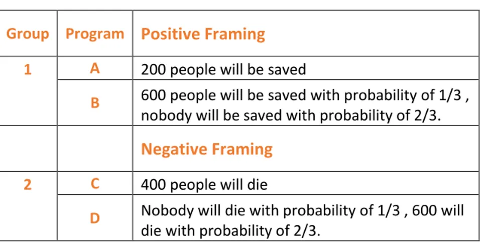
18 2.2.6. Framing:
The Framing Bias is closely related to the Prospect Theory. Kahneman and Tversky (1984), explains this bias with a well-designed study. They use two groups of people in the study and ask them to choose one of the two programs to overcome an Asian illness in US. The experiment is summarized in Table 2.2.
Table 2.2 Framing bias experiment of Kahneman and Tversky.
Group Program Positive Framing
1 A 200 people will be saved
B
600 people will be saved with probability of 1/3 , nobody will be saved with probability of 2/3.
Negative Framing
2 C 400 people will die
D
Nobody will die with probability of 1/3 , 600 will die with probability of 2/3.
Both the programs A and C and the expected value of program B and D are exactly equal. However, when the situation is framed positively, 72% of the subjects in group 1 chose program A and the rest chose B. On the other hand, when the situation is framed negatively, 22% of the subject chose program C and the rest chose D.
This experiment shows that when you describe an event with different framings, the perception in human mind might be different and they make significantly different decisions about the same subject. Describing problems with different words or illustrating the data with different charts or tables can change the perception in investors’ mind and their decisions may differ in the same situation.
19 2.3. Emotional Biases
The Emotional Biases are associated with the aspects of feelings when processing information while Cognitive Biases are associated with the type of organizing information. It is more difficult to identify and evaluate Emotional Biases. Thus, Cognitive Biases have been more analyzed in the literature. Emotional Biases that are often referred to in the behavioral finance literature are explained below.
2.3.1. Endowment Effect:
The people tend to assign greater value to an object when they own it. Professor Richard Thaler (1994)5 who also conducted an experiment with Daniel Kahneman and Jack L. Knetsch to show
Endowment Effect defines this bias as follows:
“If out-of-pocket costs are viewed as losses and opportunity costs are viewed as foregone gains, the former will be more heavily weighted.”
According to law of one price, which is one of the major assumptions of classical economic theory, a good must have a unique price at all locations. However, people give different values to the same good when they own it because of endowment bias. The willingness to pay and the willingness to accept are two different things.
Samuelson and Zeckhauser (1988) designed controlled experiments using a questionnaire consisting of a series of decision questions. The subjects were asked to choose four investment alternatives: a moderate-risk company, a high-risk company, U.S. Treasury bills and municipal bonds when they inherited a large sum of money from your great uncle. There are two versions of decision questions: neutral version and status quo6 version. In the neutral version, the four
investment alternatives are available and the subjects are free to choose. On the other hand, in
5 Thaler, R. (1994), “Quasi Rational Economics”, Russell Sage Foundation.
20 the status-quo version, the subjects were told that the inheritance was already invested in one of the investment alternatives.
The results showed that the subjects of the studies were influenced more by the status quo than by their own risk and return objectives since most of them did not change their investments in status quo version although they choose another investment alternative in neutral version.
Kahneman et al. (1990) also conducted various experiment with university students to measure endowment effect and found that short-term ownership would be enough to suppress preferences and tastes of individuals.
2.3.2. Loss Aversion:
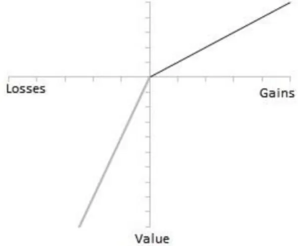
The origin of loss aversion bias is the Prospect Theory which is developed in 1979 by Kahneman and Tversky. As I mentioned in Section 2.1. , Prospect Theory states that people assign different values to gain and loss dimensions. The value functions have different characteristics on the gain/loss domains as shown in Figure 2.1.
21 The Prospect Theory states that the degree of loss aversion is greater enough to move away from the principles of expected utility theory. Pompian (2012)7 summarizes loss aversion as:
“… Loss aversion causes investors to hold their losing investments and to sell their winning ones, leading to suboptimal portfolio returns.”
Thus, Pompian creates a link between loss aversion and the Disposition Effect. The Disposition Effect will be explained below in detail.
In addition to disposition effect bias, loss aversion is seen as the main source of other irrational behaviors such as endowment effect bias or optimism since people sometimes make irrational decisions only to avoid loss. Furthermore, Shefrin and Statman (1985) investigated the aspects of loss aversion by using historical transaction data and stated that other elements, namely mental accounting, regret aversion, self-control, and tax consideration are also included in the framework that concerning a general disposition to sell winners too early and hold losers too long.
2.3.3. Regret Aversion:
If there is an uncertainty in a decision making process, regret aversion is one of the frequently observed bias after loss aversion. People mostly do not take an action to avoid regret in risky situations. For example, if they think that there is a lot of uncertainty about the future of stock’s price, they do not purchase this stock to avoid regret in the case of price decreases.
There are two aspects of regret aversion: errors of commissions (cases where people suffer because of an action they took) and errors of omission (cases where people suffer because of an action they fail to take). It is very close concept to loss aversion and Shefrin and Statman (1984) also studied on this bias and found that investors prefer stocks that pay dividends and regret is stronger for errors of commission.
They explained this findings as following: If you have to sell some of the stocks of a company that does not pay dividend and there is subsequent increase in the price of that stock, you feel
7 Pompian, M. M. (2012), “Behavioral Finance and Investor Types: Managing Behavior to Make Better Investment
22 substantial regret because the error is one of commission. Conversely, if you have to sell some of the stocks of a company that pay dividend and there is subsequent increase in the price of that stock, you feel less regret because you are able to extract cash from the dividends.
2.3.4. Disposition Effect:
It can be explained by the concepts of loss aversion and regret aversion (discussed earlier). Investors do not want to realize loss but they strongly want to realize gain. Thus, they have the tendency of selling stocks whose prices are above the purchasing price and holding stocks whose prices are below the purchasing price. There is extremely large literature about this bias including both field experiments and controlled laboratory experiments.
Firstly, Weber and Camerer (1998), proved the existence of Disposition effect by conducting controlled laboratory experiment with university students in Germany. Their findings showed strong evidence on the existence of Disposition Effect: “Subjects will tend to sell winners and keep losers.”
On the other hand, Odean (1998)8 analyzed transactions of 10.000 investors at a large discount
brokerage firm between 1987 and 1993 and stated that: “… individual investors demonstrate a significant preference for selling winners and holding losers, except in December when tax motivated selling prevails.”
There is also demographic-based research that try to relate this bias with gender. Da Costa et al. (2008), found that the hypothesis about the existence of Disposition Effect collapse for female subjects when the reference point is the previous price instead of purchasing price. (Hypothesis: Subjects sell more (less) stocks when the sale price is above (below) the previous price).
Many researchers discuss the dimensions of this bias in terms of time horizons. For instance, Svedsater et al.(2009) claimed that Disposition Effect and feedback strategy have different roles depending on the time period. Investors have different perceptions in long-run and short-run and the probability to have that type of bias increases as the time period increases. In addition,
23 Risfandy and Hanafi (2014)9 stated that “Investors behave as momentum trading when respond
to short-run return and became contrarian trader when they react to long-run return”. Disposition Effect exists clearly in the long-run.
My research also makes a contribution to Behavioral Finance literature especially in the context of Disposition Effect. However, my approach is quite different from the previous ones and will be explained in detail in Section 3.
2.3.5. Self-Control:
The classical consumption theory, which is called Life-Cycle Hypothesis (LCH), assumes that people want to smooth their wealth during their life, so they save significant amount of their earnings of today to keep their standards of living continuous. According to LCH, there is no attraction of consumption for today. However, behavioral theory claims that people prefer to consume today rather than save for tomorrow. There is a strong attraction to consume today and this is self-control bias.
The Self-control bias was firstly introduced by Shefrin and Thaler (1988) and they state that self-control underlies national borrowing/savings rate.
Erdem and Can (2013) conducted a survey to check present-bias as well as self-control problems among individuals in Turkey and found that in particular, the low-income and old-age individuals suffer present-bias problem. Thus, the failure in savings can also be explained by behavioral aspects of decision making.
2.3.6. Optimism:
Optimism is the belief and feeling that things have a good chance to come out favorably. Optimist investors think that their investment decisions are not affected from bad things and investment tools they chose are always the best. Thus, they are not interested in decreasing risk by diversification. This bias makes their portfolio potentially vulnerable.
9 Risfandy, T. and M. M. Hanafi (2014), “An Experimental Study on Disposition Effect: Psychological Biases, Trading
24 The optimism bias can cause investors to see themselves as above the average and lead investors to make irrational decisions because the investors are optimist about the progress of the market, progress of the overall economy and the potential performance of the investment.
Montier (2002) explains optimism as: “Perhaps the best documented of all psychological errors is the tendency to be over-optimistic. People tend to exaggerate their own abilities. Like the children of Lake Woebegone, they are all above average. For instance, when asked if they thought they were good drivers, around 80% of people say yes!”
In summary, both cognitive biases and emotional biases have common aspects and they share illogical facts of human beings. However, each of them can explain exactly one aspect of irrationality in decision making process. In this study, DE can be clearly seen in the behaviors of individual investors and it is investigated at a broader context including the effects of demographic features such as gender and age.
2.4. Buy-Sell Imbalance
The Buy-sell imbalance (BSI) is a ratio of net buying value to the total trading value and it is used as a measurement tool, especially to analyze buying behavior of investors in financial markets. Irrationality on the behaviors of investors breakdowns the basic assumptions of classical finance theory and creates inefficiency in the market since the systematic irrational behavior which is called ‘bias’ or ‘anomaly’ provide others - especially professional market makers - to obtain an unfair advantage by using the anomalies in a systematic way. Thus, investigating the behaviors of the investors and clarifying the reasons of them issubstantially important to achieve an efficient and fair financial market.
In the earlier studies, classification of transactions was not publicly available, so researchers developed methods to classify buyer-initiated or seller-initiated trades through the whole transactions. The most frequently used method is the algorithm of Lee and Ready (1991) which
25 defines the type of transaction (buy or sell) referring to the time between order of a transaction and realization of a transaction.
Chordia et al. (2002), use the term ‘OIBNUM’ as the number of buyer-initiated trades less the number of seller-initiated trades on a daily basis. Each transaction is determined whether it is buyer-initiated or seller-initiated transaction using the Lee and Ready algorithm and calculate stock-based order imbalance using historical transactions of US individual investors. They try to identify the direction of feedback trading strategy and the persistency of this strategy by regressing OIBNUM on day-of-the-week dummies, past lagged values of market return and also past lagged values of order imbalance (S&P500 Index is used as an aggregate market index). As a result, they found that investors use contrarian feedback strategy; they buy when the market declines and sell when the market rises. The validity period of contrarian strategy is just three days.
Kamesaka et al. (2003), on the other hand, calculates ‘Net Investment Flow (NIF)’ for each investor group as purchasing value minus selling value divided by total trading value on a weekly basis. Their investor groups consist of individual investors, foreign investors and five types of institutional investors. Vector Autoregression (VAR) Model is implemented for each investor group using NIF and Tokyo Stock Price Index (Topix) return as a dependent variables to test for Granger causality between investor group trading and market returns. Also, to study the performance of investor groups after heavy buying and selling weeks, they divide each group into five equal sets. The Group 1 contains the weeks of highest positive NIF and called buy weeks, and the group 5 contains the weeks of largest negative weeks and called sell weeks. For each group, the average market return for the next period is analyzed to examine portfolio performance of each investor groups. The term ‘period’ is used to represent three different time horizons that are: one week, one month and two months. As a result, they stated that “After taking into account investment flow autocorrelation using the bivariate VAR(4) model, foreign investors, companies, and Japanese individual investors appear to be short-term positive feedback traders.” Positive feedback trading means that, these investor groups buy after the market rises and sell after the market declines. On the contrary, banks, insurance firms, and investment trusts follow negative feedback trading strategy. Furthermore, they also analyzed portfolio performance and
26 found that there is no exact relation between feedback trading strategy and portfolio performance.
Griffin et al. (2003), also try to investigate the relation between previous term return and current buy-sell imbalance. They stated that: “On the day following extreme return performance, stocks in the top decile of firm performance are 23.9% more likely to be bought in net by institutions (and sold by individuals) than those in the bottom decile of return performance”. Price increase in a stock is a buy signal for institutional investors while the same movement is a sell signal for individual investors. This result also shows that institutional investors are less affected by Disposition Effect bias than individual investors. They also found that return movements can not be predicted by using trade imbalance at the daily frequency.
Kumar and Lee (2006), have studied with the data of large discount brokerage firm in the US and calculate two types of BSI: first one is monthly portfolio BSI which is well-known measurement for investor sentiment and second one is monthly investor BSI which is more similar to our measurement method. However, they stated that portfolio based BSI and investor based BSI generates similar results about herding behavior so it is unnecessary to analyze both of them and they continue to the analysis with portfolio based BSI. They also perform time series regression by regressing portfolio BSI on unexpected inflation, monthly growth in industrial production, change in the term spread, change in the risk premium, monthly unemployment rate and innovations in average hourly earnings and lastly they added expected future cash flows as an explanatory variable. They conclude that “Even though changes in retail sentiment are likely to be partially induced by innovations in macroeconomic variables, the residual retail sentiment changes as captured by the residual BSI measure have considerable incremental power for explaining comovements in small-cap stock returns.”
Colwell et al. (2008), studied the impact of the trading imbalances of investor categories on stock returns in Australian stock market. They calculated time series of BSI for each stock aggregated by investor groups. Stock-based BSI is calculated as the number of shares of stock purchased minus the number of shares of stock sold divided by the total number of shares of stock traded. Bivariate VAR analysis is used to investigate the Granger-causality between BSI (for each stock
27 and for each investor category) and stock returns lagged up to one week (include 5 lags). They also repeated the analysis with weekly data for 4 lags and that extend the analysis to one month. They found that Granger-causality between stock-based BSI and stock return exists both at daily and weekly intervals. However, only individual investors have the tendency to sell the stock after price increases which is referred to negative feedback strategy and also an evidence of Disposition Effect bias. Other categories such as institutional investors or foreign investors do not follow negative feedback trading strategy exactly.
Barber and Odean (2008), claimed that investors have limited attention when they make buying/selling decisions and attention-grabbing stocks are bought more rather than others. They defined three proxies for attention which are trading volume, return and news and calculate stock based BSI for each group of stocks to measure the net buying ratio.
First, they calculated abnormal trading volume as the ratio of the stock’s trading volume of the day to its average trading volume over the previous one year and stated that if the stocks have higher abnormal trading volume, it is the signal of attention and these stocks are bought more than others. Second, they calculated previous day returns of each stock and stated that if the stocks have higher previous day return, it is also the signal of attention and these stocks are bought more. Lastly, they divided stocks whether the company’s name is on the Fortune 500 at that day or not and stated that if the daily news contain the company’s name, it is the signal of attention and these stocks are also bought more. Also, they calculated stock based BSI for each group of stocks to measure the net buying ratio.
Actually, the second proxy; ‘return’ is the related one to my research. Odean and Barber found that previous day return of a stock is a strong proxy of attention and buying ratio of that type of stocks is significantly higher especially for individual investors but there is u-shaped relation between them. The value imbalance is 29.07 for the largest negative return group (according to the return of previous day) and 11.13 for the highest positive return group while it is around -7 for the middle return group. On the other hand, institutional investors generally do not follow this pattern meaning that they are not affected from Disposition Effect Bias as a whole as individual investors affected.
28 Overall, BSI is calculated either based on stocks (the ratio of net buying to the total trading of a particular stock) or by summing up all purchasing and selling transactions of a particular investor group in the earlier studies. This type of ratio can only provide limited knowledge about the behavior of an investor. However, BSI; calculated in this paper can provide direct and obvious knowledge since it is calculated for each investor separately as the ratio of net buying value to the total trading value of an investor. This is the first paper in which investor behavior is investigated by using investor-based BSI which is calculated on a daily basis for each investor. In this study, the focus group is only individual investors since it was proved in the earlier studies that DE is clearly seen on the behaviors of individual investors not of institutional investors.
3. Data & Methodology
3.1. Data
The actual source of the data is Central Registry Agency (MKK) which electronically keeps all the historical data which belongs to capital markets.
The data includes approximately 25.000 individual investors’ transactions that were selected according to the following criteria:
Investors having portfolio amount more than TRY 1.000 (or USD 500)
Investors making at least one transaction in between the sampling period.
The selection of the data is preserved under stratified random data characteristics such as the age, portfolio size distribution of the sample is the same in the population.
The sampling period is between 01.01.2008 and 31.12.2012 and the data includes approximately 1259 observations of non-holiday regular weekdays.
The data consists of daily transaction values, transaction types as buy or sell, transaction name as stock names and balance of portfolio for each investors in which investors are defined as numbers because of privacy policy. In addition to transaction details, gender and age of investors are also known as a demographic information.
29 Two other variables are also derived from the data which are buy-sell imbalance and market-adjusted portfolio return (the derivation methods will be explained in Section 3.2.). All variables used in statistical analysis and regression analysis are available on a daily basis.
3.1.1. Descriptive Statistics
The whole data consists of approximately 31,475,000 observations for each variable since there are 25,000 investors and 1259 days. The investor data consists of 18947 males and 6049 females. The distribution of investors based on gender, which is summarized in Figure 3.1. as percentage values, is consistent with the population of Turkey’s financial market since 26% of individual investors who are trading in Borsa İstanbul are female investors and 74% of them are male investors according to 2013 statistics of MKK.
Figure 3.1 The distribution of the investors based on gender.
Men 76% Women 24%
Gender Distribution
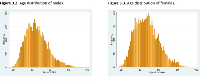
Men Women30 Figure 3.2. Age distribution of males. Figure 3.3. Age distribution of females.
The age distributions of males and females are positively skewed and the distributions are demonstrated on the Figure 3.2 and the Figure 3.3. The details about the age of investors are summarized in the Table 3.1
Table 3.1 Descriptive statistics of the investors’ age.
Statistics: Age No. of observation 24996 Mean 46 Median 45 Variance 149.12 Skewness 0.59 Kurtosis 3.17
The investors are divided into two subsamples as male and female and three age intervals which represent young adults, middle age and old investors that are created for both male and female investors. The age intervals are 18-35 for young adults, 36-55 for middle-aged adults and 56+ for old investors.10
Descriptive statistics of other variables (BSI and market-adjusted portfolio return) will be displayed at the next section after the explanations about the derivation processes.
10 Information about the age of investors, which are collected from MKK, represents the age in 2008 and they are
31 3.2. Methodology
Mainly, there are two different analysis in this paper: statistical analysis and regression analysis. They are independent analysis in terms of implementation but produce closely related results. Two other variables (Buy-sell imbalance and market-adjusted portfolio return) are derived from the data collected from MKK in order to complete these analysis. Buy-sell imbalance is the widely used ratio to measure buying appetite and market-adjusted portfolio return is derived to display the relationship between previous day return and buying appetite of investors. Detailed explanation about derivation process is described below. Also, the model specification process for the regression analysis is driven with the help of conducted studies with panel data.11
1) Buy-sell imbalance:
It is calculated for each investor on a daily basis as the difference between purchasing value of all stocks, and selling value of all stocks in a given day divided by the sum of purchasing value of all stocks and selling value of all stocks in a given day. The value is calculated by multiplying price of that stock and quantity purchased or sold in a given day.
, , , , , , 1 1 , , , 1 1 i t i t i t i t s s i t i t i i j t s s i t i t i i P V S V B S I P V S V
where, , , , p i t i t i t P V Q P and S Vi t, Qi ts, Pi t, , j tB S I is the buy-sell imbalance of investor j on day t, P Vi t, is the purchasing value of stock i on day t and S Vi t, is the selling value of stock i on day t. ,
p i t
Q is quantity purchased on stock i on day
11 Erdem, O. and Y. Varlı (2014), “Understanding the Sovereign credit ratings of emerging markets”, Emerging
32
t, ,
s i t
Q is quantity sold on stock i on day t and Pi t, is the price of that stock on day t. si t, is the number of stocks purchased or sold on day t.
,
j t
B S I is a ratio between -1 and 1. If it is equal to -1, it means that investor does not buy anything, but instead sells stock(s). This action indicates the decrease in the buying appetite. If it is equal to 1, it means that the investor does not sell anything, but buys stock(s). That action indicates the increase buying appetite. If it is equal to 0, either investor does not buy or sell anything or the purchasing value and selling value of stock(s) are exactly the same.
BSI is usually calculated as the buy-sell imbalance of a stock rather than of an investor in the earlier studies. However, it is calculated for each investor to measure the buying appetite of investors separately, in this paper. This is the first important contribution of this paper, since the investor-based BSI provides direct knowledge about the investor’s behaviors.
2) Market-adjusted portfolio return:
, , , , , 1 . j t s m j t i j t i t t i r p r r
, j tr is the market-adjusted portfolio return for investor j on day t, pi j t, , is the weight that is calculated by dividing the end-of-day market value for stock i to the end-of-day market value of portfolio held by investor j on day t, ri t, is daily return for stock i on day t, sj t, is the number of
stocks held by investor j on day t and m t
r is corresponding daily rate of return on BIST100 index.
Descriptive statistics of above two variables (buy-sell imbalance and market-adjusted portfolio return) are summarized at Table 3.2.
33 Table 3.2 Descriptive statistics of the buy-sell imbalance (BSI) and the market-adjusted portfolio return based on
investor types.
Buy-sell imbalance (BSI) Market-adjusted portfolio return Male Mean 0.0052 0.01% Median 0 -0.09% Variance 0.0473 0.0005 Female Mean 0.0014 0.02% Median 0 -0.07% Variance 0.0267 0.0004 Young Mean 0.0086 0.01% Median 0 -0.12% Variance 0.0590 0.0006 Old Mean 0.0021 0.01% Median 0 -0.06% Variance 0.0348 0.0004
Note: There are 6049 female and 18947 male investors. 5243 of them are young and 5167 of them are old investors. Market-adjusted portfolio return exists for the days in which the investor makes any trading (buy-or sell) for each investor. BSI exists independent of whether or not there is any trading.
3.2.1. Statistical Analysis
In this section, there are two types of analysis: First one shows the general relation between the buying appetite of investors which is evaluated with BSI and previous portfolio return, while the second gives detailed information about this relation based on investor categories.
In order to see the major link between portfolio return and BSI, similar methodology of Barber and Odean (2008)12 is implemented. Individual investors are sorted according to their previous
day return and divided into five groups each of which has equal number of observations. This grouping operation is repeated for each day in the sampling period. Each day, there are five groups but the investors in these groups may change according to their previous day’s returns. Then, the average BSI values of each group are calculated for each day (Average means average
12 Barber, B. and T. Odean (2008), “All That Glitters: The Effect of Attention and News on the Buying Behavior of
Individual and Institutional Investors”, Review of Financial Studies, 21(2):785-818. Methodology was explained at Section 2.4.
34 BSI values of investors in the group). At the end of this process, five time series data, which contain average BSI values are created. The first series represents the loser group which consists of market loser investors based on previous day portfolio returns while the fifth series represents the winner group that consists of market winner investors based on previous day portfolio returns. The following formula summarizes the process explained above.
, , 1 , , p t n j t j p t p t B S I B S I n
, p tB S I is the buy-sell imbalance of group p on day t, B S Ij t, is the buy-sell imbalance of investor j on day t and np t, is the number of investors in group p, where p=1,…,5. If p is equal to one, it
means that the group consists of market losers and if p is equal to five, it means that the group consists of market winners.
As explained in previous section, BSI is seen as a measure of buying appetite. It is between -1 and 1. If it is equal to -1, it means that investor does not buy anything but sell stock(s). This action indicates decreasing buying appetite. If it is equal to 1, it means that investor does not sell anything but buy stock(s). That action indicates increasing buying appetite. If it is equal to 0, either investor does not buy or sell anything or the purchasing value and selling value of stock(s) are exactly the same.
Furthermore, in order to see the effects of demographic features within this context, individual investors are divided into subsamples based on ages and gender. The same procedure of grouping and averaging which are explained above are implemented into these subsamples to see whether there is a difference between buying appetites of different investor categories. Detailed results are demonstrated at Section 4.
35 3.2.2. Regression Analysis
In order to determine the effect of previous return and demographics on BSI, the panel regression is performed with the transactions of the whole investors between 2008 and 2012 and the investor is defined as a panel variable. BSI is regressed on the previous day market-adjusted portfolio return (rj t,1), exchange rate (x rj t, : TRY/USD is used as a representative substitute of
stock investment in Turkey) and three types of dummy variables that are used to measure the effect of gender and age on BSI. The simple linear regression model:
, 0 1 , 1 2 , 3 4 5 ,
j t j t j t j t
B S I r x r f e m a l e m i d d l e o l d u
, 1
j t
r represents the market-adjusted portfolio return of investor j on day t-1 and it is assumed to be stationary by the nature of return. BSI is also stationary series since it is strictly bounded with -1 and 1. However, exchange rate is nonstationary series, so the first difference is calculated to make it stationary and it is represented as x rj t, in the equation (Stationarity is checked with ADF
test13). Also, there are three dummy variables: female, middle and old. First one is gender dummy
and it takes 1 for female investors and 0 for male investors. The second one is age dummy for middle age investors. It takes 1 for middle age investors and 0 for others. Last one is also age dummy for the old investors and it takes 1 for old investors and 0 for others. Young adult investors is determined as reference category in this model and age intervals are defined the same as in the statistical analysis.
As a first step, the above model is used as a simple linear regression model with panel data which is called pooled OLS. Also, pooled OLS with cluster robust standard errors model is also implemented to see whether there is a correlation between explanatory variables and residuals. However, there is autocorrelation in residuals and it is proved by Wooldridge test which is used to test serial correlation in residuals in panel data.
36 Thus, fixed and random effect linear models with AR(1) disturbance term are used to analyze panel specific effects by assuming first order autocorrelation in residuals. The assumptions of the fixed effect model as following:
, ,
j t j j t
u
,
j t
u is the disturbance term of the regression and assumed to satisfy usual conditions of linear regression. j represents individual-specific, time invariant effects which are gender and age in this study, j t, represents both individual and time specific effects. Also the following
assumptions exist in the model with random effect.
j
̰ ~ i.i.d. N
0 , 2
and j t, ~ i.i.d. N
0 ,2
According to fixed effect model, individual specific error terms are assumed to be fixed, but the effect of time invariant variables such as gender and age can not be seen because of collinearity. Although the Hausman specification test suggest that fixed effect model should be used, the random effect model is also employed to see the effect of time invariant variables.
4. Results
4.1. Statistical Results
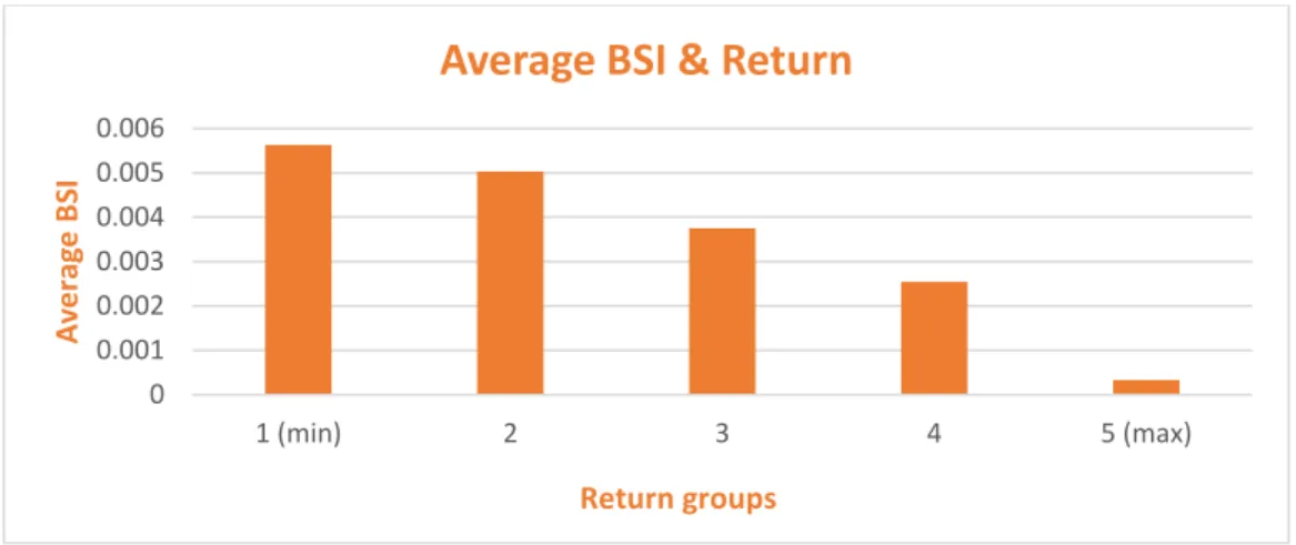
Before dividing individuals into categories, we perform extensive analysis which gives a wider picture about the behaviors of all individual investors. Figure 4.1 indicates the result of this primary analysis. Group 1 represents minimum return group and group 5 represents maximum return group. Average BSI is positive but decreasing as previous day portfolio return increases meaning that buying appetite and portfolio returns are negatively correlated. These findings are consistent with the earlier studies on DE (Weber and Camerer; 1998, Odean; 1998, Costa et al; 2008, Svedsater et al; 2009, Talpsepp; 2010).
37 Figure 4.1 The relationship between the average BSI and previous day market-adjusted portfolio return.
Note: Investors are sorted based on previous day portfolio returns and divided into 5 groups. Group 1 consists of investors whose previous day portfolio returns are minimum. Group 5, on the contrary, consists of investors whose previous day portfolio returns are maximum. In each group, there are approximately 5,000 investors.
Below table (Table 4.1) shows the details of group variables. First two groups include market loser investors whose previous day market-adjusted portfolio returns are negative. Group 3 includes market neutrals who have both negative and positive market-adjusted portfolio returns but they are very close to zero meaning that their return is almost equal to the market return. Last two groups are market winners whose previous day portfolio returns are positive. Each group has approximately equal number of observations (investors).
Table 4.1 The comparison of the average BSI values of each group for all investors. Return Groups Minimum Return Maximum Return Average Return Average BSI t value t value for the group: 1 (min) -0.66428% -0.01224% -0.02480% 0.00563 1.65921* 1 and 2 2 -0.01224% -0.00408% -0.00780% 0.00503 3.10460*** 2 and 3 3 -0.00408% 0.00232% -0.00088% 0.00375 2.84393*** 3 and 4 4 0.00232% 0.01102% 0.00620% 0.00254 5.56300*** 4 and 5 5 (max) 0.01102% 4.93202% 0.02787% 0.00033 15.03214*** 1 and 5
Note: The t statistics belong to BSI series.*** refers to significance at 1%, ** refers to significance at 5%, * refers to significance at 10%.
As seen from the table, the previous day’s return significantly affects current day’s buying/selling decisions. For the minimum return group, average BSI, which is a measure of buying appetite, is
0 0.001 0.002 0.003 0.004 0.005 0.006 1 (min) 2 3 4 5 (max) A ve rag e B SI Return groups
38 0.00563, while it is 0.00033 for the maximum return group. The test results indicate that there is a significant difference between the return groups. To compare the maximum and minimum return group, t statistic is 15.03214 which is sufficiently high to reject the hypothesis that the average BSI of investors in minimum return group is equal to the average BSI of investors in maximum return group. To summarize, the investors realize gains while they avoid to realize losses since they sell the stocks (meaning that BSI is lower) the day after they won (if market adjusted portfolio return of an investor is positive, it means that he/she has won), but they do not sell the stocks the day after they lost (if market adjusted portfolio return of an investor is negative, it means that he/she has lost). This is a strong evidence on the existence of Disposition Effect bias.
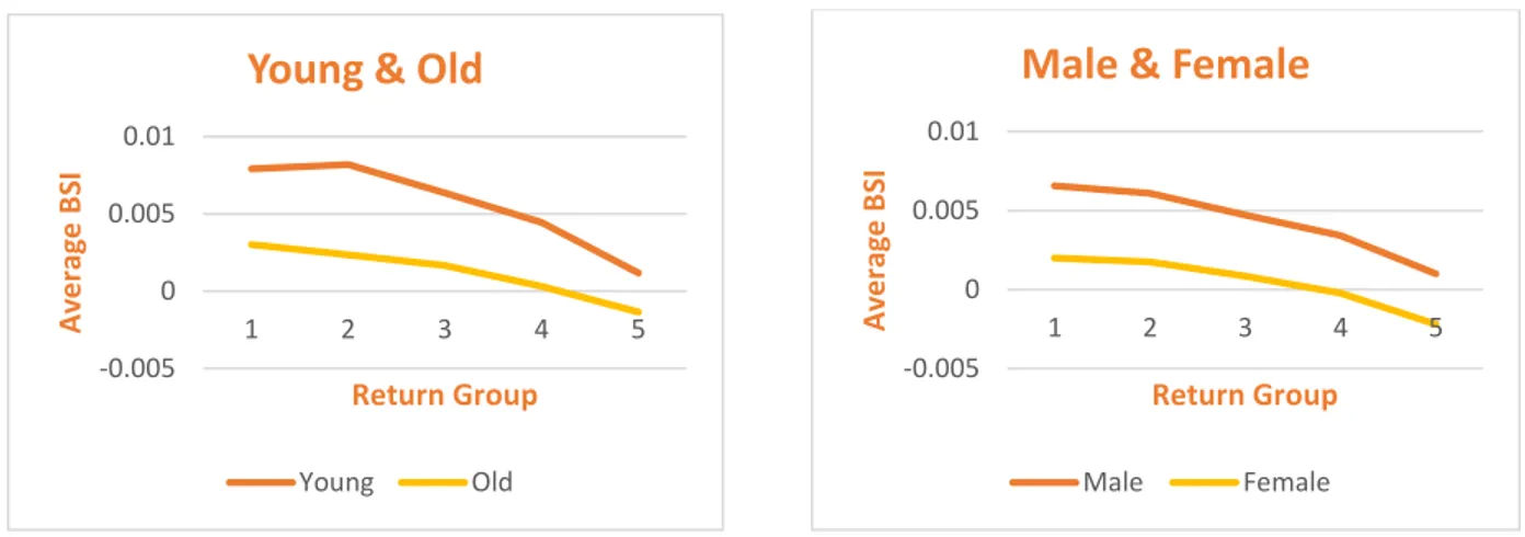
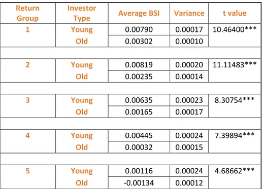
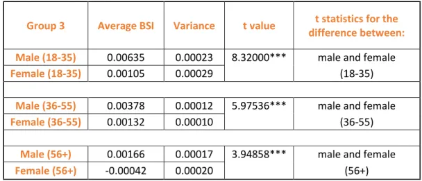
After proving the existence of the bias, the analysis is expanded into investor categories that are explained in descriptive statistics section. The same procedure of grouping and averaging are implied to each investor category. Below figures shows the relationship between level of influence from this bias and demographics (age and gender).
Figure 4.2 Comparison of young and old investors. Figure 4.3 Comparison of male and female investors.
Note: The entire data divided into two subsamples based on both age and gender. In order to provide more obvious results based on age, the middle age is dropped14.
14 Detailed results including middle-age are provided on Appendix - Part A.
-0.005 0 0.005 0.01 1 2 3 4 5 A ve rag e B SI Return Group
Young & Old
Young Old -0.005 0 0.005 0.01 1 2 3 4 5 A ve rag e B SI Return Group