An index structure for moving objects in video databases

ш м DC І Т І Ш І

Ш

Ш

Ш ^ Ш

Я- O ' hÊÊ0Î J“m il' •^¿>-ЛЁЁ^>Гт 'чіі0'Щді‘-<ц0г

J

i

AN INDEX STRUCTURE FOR MOVING OBJECTS

IN VIDEO DATABASES

A THESIS

SUBMITTED TO THE DEPARTMENT OF COMPUTER

ENGINEERING AND INFORMATION SCIENCE

AND THE INSTITUTE OF ENGINEERING AND SCIENCE

OF BILKENT UNIVERSITY

IN PARTIAL FULFILLMENT OF THE REQUIREMENTS

FOR THE DEGREE OF

MASTER OF SCIENCE

By

Tuba Yavuz

August, 1999

■іЯ -!6·<3“ί·

I certify that I have read this thesis and that in my opin­ ion it is fully adequate, in scope and in quality, as a thesis lor the degree of Master of Science.

Assoc. Pr:'OK Dr. Ozgiir U lu ^y(P rin cipal Advisor)

I certify that 1 have read this thesis and that in my opin­ ion it is fully adequate, in scope and in quality, as a thesis for the degree of Master of Science.

^ 1 .

Asst. ' ’ r o l D r .^ g u r Güdükbay

I certify that I have read this thesis and that in my opin­ ion it is fully adequate, in scope and in qiuility, as a thesis for the degree of Master of Science.

A

Assii. Prof. )0r.l A ttila GiirJdy

Approved lor the Institute of Engineering and Science:

<r

Ill

A B ST R A C T

A N IN D E X S T R U C T U R E F O R M O V IN G O B J E C T S IN V ID E O D A T A B A S E S

Tuba Yavuz

M .S. in Computer Engineering and Infornuition S Supervisor: Assoc. Prof. Dr. Özgür Ulusoy

August, 1999

ce

Modeling moving objects and Iiandling various types of motion queries are interesting topics to investigate in the area of video databases. In one type of motion queries, motion of multiple objects is specified by the changes in relative spatial positions of objects. Answering such kind of queries, that involve motion of multiple objects whose identifications cire not specified, requires some type of indexing because the time complexity of processing such a query in the absence of an index structure is

0 {N \ l{N —

N

n

SMIST-'mdex

SMIST-'mdex

Key words:

IV

ÖZET

V İD E O V E R İ T A B A N L A R IN D A H A R E K E T E D E N N E S N E L E R İÇİN B İR İN D E K S Y A P IS I

Tuba Yavuz

Bilgisayar ve Enformatik Mühendisliği, Yüksek Lisans Tez Yöneticisi: Doç. Dr. Özgür Ulusoy

Ağustos, 1999

Video veri tabanı alanında, hareketli nesnelerin modellenmesi ve çeşitli hareket sorgularının cevaplanması oldukça ilgi çeken bir araştırma konusu olmuştur. Hareket sorgularının bir çeşidinde birden fazla nesnenin hareketleri birbirlerine göre olan yerlerindeki değişiklikle ifade edilmektedir. Birbirlerine göre uzay- sal ilişkileri belirtilmiş fakat kimlikleri belirtilmemiş nesnelerden oluşan bu tip sorguların cevaplanması özel bir indeks yapısının kullanılmasını gerektirir. Bunun nedeni, böyle bir sorgunun herhangi bir indeks yapısı kullanılmaksızın cevaplanmasmın hesaplama karmaşıklığı

0 {N \ l{N — n)\)

N

SMlST-indeks

SMIST-indeks

Anahtar kelimeler:

D e d ic a t e d to

my parents C a h id e and M u s t a f a Y a v u z , my brothers O s m a n Y ü k s e l and E m r e , and my husband T a m e r K a h v e c i.

VI

A C K N O W L E D G M E N T S

First of all, I would like to express iny gratitude to Assoc. Prof. Özgür Ulusoy for his patient supervision and invaluable guidance. I would like to thcink Kasirn Selçuk Cfindan for his invaluable comments. 1 am gi'citefnl to Asst. Prof. Uğur Güdükbay and Asst. Prof. A ttila Gürsoy for reading this thesis and their comments. 1 would also like to mention the support and sacrifice of my family. Finally, I would like to thank my friend Kadriye Özba.ş for her moral support.

Contents

1 I n t r o d u c tio n 1

2 R e la t e d W o r k 4

2.1 A Framework for Querying Structural S im ila r ity ... 7

3 I n d e x C r e a tio n 1 5

3.1 Spatial O rg c in iz a tio n ... 1,5

3.1.1 Spatial R epresentcition... 16

3.1.2 Spatial P artition in g... 18

3.2 Temporal O rg a n iza tio n ... 21

4 Q u e r y E x e c u t io n 2 7

4.1 An Algorithm for Query E x e c u t i o n ... 29

5 I m p le m e n t a t io n D e t a ils 3 3

6 E x p e r im e n t s 3 8

7 C o n c lu s io n a n d F u tu r e W o r k 4 9

List of Figures

2.1 Nine region of interest, for ID relation representation 8

2.2 Relative positioning of the intervals [3,8] and [ 5 , 7 ] ... 8

2.3 The algorithm for finding the distance between two ID relations 9

2.4 Instantiation a lg o r ith m ... 10

2.5

Check Forward

2.6

Join window reduction

3.1 D ata for moving objects

a, b, c,

d

3.2 Spatio-temporal relations for data in Figure 3.1 19

3.3 The cilgorithm for production of

maximal sets

3.4 Tim e intervals of

Spatio-temporal relations

3.5 Tim e intervals of

Spatio-temporal relations

3.6 T im e intervals of

Spatio-temporal relations

3.7 Tim e intervals of

Spatio-temporal relations

4.1 An example of the first frame of a structural query 29

4.2 An cilgorithm for constructing the match set of each object . . . 30

LIST OF FIGURES

5.1 A sample R D -t r e e ... .35

5.2 An algorithm for constructing the match set of eci.ch object by using the

relation set

6.1 Disk accesses as a function of number of objects in the database 41

6.2 Disk accesses with

SMIST-hidex

List of Tables

2.1 Internal node bounding condition for left most b i t ... 12

2.2 Internal node bounding condition for right most b i t ... 12

2.3 Leaf node bounding condition for left most b i t ... 13

2.4 Lecif node bouirding condition for right most b i t ... 13

2.5 Domain window bound conditions for left most bit 13 2.6 Domain window bound conditions for right most b i t ... 14

3.1 Interval R elationships... 16

3.2 Definition of Directional R ela tio n s... 18

3.3 Definition of Topological Relations 20 3.4

SMIST-uidex

3.5 M axim al sets and corresponding common time intervals for di.sjoint-w e s t ... 23

3.6 M axim al sets and corresponding common time intervals for disjoint-north ... 25

3.7 M aximal sets and corresponding common time intervals for di,sjoint-n o r t h w e s t ... 26

LIST OF TABLES

3.8 M axim al sets and corresponding common time intervals lor disjoint-

northeast 26

4.1 First object and Second object sets lor each valid time interval [s, e] and topological directional rehition

tdi

4.2 M atch sets for each object for each valid time interval [s, e] and topological-directioiicil relation

t d i

4.3 Filled matchset for each object for each valid time interval [s, e] . 32

4.4 Possible matches for each valid time interval [s, e ] ... 32

5.1

Relation sets

5.2

Relation sets

5.3

Relation sets

5.4

Relation sets

5.5 Matchset for each object for each valid time interved [s,

e] . . . .

6.1 Number of disk accesses performed with

SMIST-mdeyi

JWR

6.2 Number of disk accesses performed in the filter step... 44

6.3 Average number of files recid for each valid tiine interval... 46

6.4 Number of valid time intervals found in during the filter stej). 47

6.5 Number of disk accesses performed with

SMIST-\n<\ex

LIST OF TABLES

_Xll

6.6 Number of disk accesses performed in the filter step for Vcxrying number of frames. Number of objects in the databct.se is 50 and number of objects in the query is 10... 47

6.7 Number of valid time intervals detected for Vcirying number of fi'cimes. Number of objects in the database is 50 and number of

objects in the query is 10. 48

6.8 Number of valid intervals found in the filter step. Number of frcirnes=100 and number of o b je c ts= 1 0 ... 48

6.9 Number of matches performed compared with possible number of matches for queries with varying number of objects. Number

Chapter 1

Introduction

The tyi^e of data stored in database systems is no longer only alphanumeric but also image, audio and video. This is the natui’cd consequence of emerging use of multimedia database systems in application dorriciins such as surveil­ lance systems, medicine, entertainment, and educcition. However, since new data types bring their own requirements such as large storage requirement and excessive content processing, in order to achieve effective use of multimedia data a number of design issues such as data modeling, query formulation, a.nd efiicient retrieval should be reconsidered.

M ultimedia data requires excessive processing and a detailed modeling of its content. This is because it is rich in content and this fact is also stressed by the well-known sciying “A picture worths a thousand words” .

Two main approaches have been followed for retrieval of multimedia da.ta. These approaches are Ccilled

annotation-based retrieval

content-based re­

trieval.

Multimedici objects, such as images, have many different attributes that could be of interest-there is no way that any tag could hope to Ccipture them all. The trick, in any cipplication context, is to identify commonly used characterizcitions and to build tags based on these.

CHAPTER 1. INTROD UCTION

Even so, there is loss of information.

The iDaper concludes that queries should be posed to objects themselves not to the tags. To put in other words, retrieval should be by content. Researchers, having realized the need for content-based retrieval, have developed various systems providing content-based retrieval of multimedia data. Some examples are [13], [1], cind [8].

Content-based retrieval is a huge research area, which ha.s a numl:)er of com ­ ponents such as preprocessing, delta modeling, and indexing. The work pre­ sented in this thesis corresponds to content-based indexing lor video databases. W e propose a new spatio-temporal index structure. Such an index can facil­ itate answering queries in which the motion of multiple objects is defined in terms of the change in objects’ relative spatial positions and the identities of the objects are undefined. W e compare the performance of our query execution model that uses the proposed index structure with the framework presented in [9], which is the only work that deals with the same type of query as the one we are interested in our work.

In [18], Papadias et al. used binary string encoding scheme for 1-D rehitions. The scheme allows automatic derivation of similarity degree between spatial structures. Structural similarity queries are handled using this scheme. R *- trees are used as the index structure. A constraint Scitisfaction algorithm, which is called

forward checking with variable reordering

In our work, we propose a new spatio-temporal index structure which is bcised on B-1—trees. W e use topological-directional relations to represent the spatial relations between objects. The index structure we propose organizes the search space first according to spatial dimension cUid then according to temporal dimension. W e also propose a query execution algorithm that uses our index structure efficiently. The algorithm consists of a filter step and a refine step. In the filter step, by using the spatial constraints in the query, time intervals that possibly include answer(s) to the query are selected. Then in the

CHAPTER 1. INTRODUCTION

refine step, the datci corresi^onding to the filtered time intervals is analyzed and all the S23atial constraints are checked to find exact matches.

The rest of the thesis is organized as follows. In Chcipter 2, we sum m a­ rize the related work. The new index structure we jDi'opose is explained in detail in Chai^ter 3. Chaf)ter 4 describes the algorithm we developed for query execution. Implementation details are explained in Chapter 5. Experimental settings and the results obtained are provided in Chapter 6. Finally, in Chapter 7 conclusions and future work are discussed.

Chapter 2

Related Work

Modeling moving objects has attracted attention of researchers sjnce motion of objects can serve as a valuable source of information that can be used to handle video sequences in multimedia databases. M ajority of the work that has been done on motion analysis belongs to the signal processing field. The research in this field has enabled shot change detection [7], video segmentation [4], [17], [20], [21], camera motion extraction [2], [15], [7], and tracking moving objects [7] which provides valuable information that can be used for answering queries of video database users regarding motion.

Apart from these studies which focus on preprocessing of raw data to extract information regarding motion, there has also been research on modeling moving objects [10], [14], motion query formulation [1], and spatial indexing lor motion queries [18].

In [10], Dimitrova et al. focus on both recovery of motion inlbrmation and its use for classification and query processing. Therefore, their work covers both motion cinalysis in digital video and information modeling and retrieval, liesides storing physiccil information of video, they use the spatial and temporal properties of objects to derive the conceptucil video data type. They define an algebraic model for rnultjmedia data. In addition, their model is comi^leted with an cilgebraic query language called E V A . EVA has the ability to deal with spatial and temporal dimensions of multimedia objects. As a result users

can formulate queries regarding motion of objects using E V A . The authors think that a knowledge-base, which includes all necessary rules, constrciints and procedures, should be used to associate object trajectory representcitions, which is obtained as a I'esult of the low-level motion analysis steps (motion detection and motion tracing), with the domain dependent “activities” . For instance, for an cipplication domain which includes only Ccirs as the moving ol)jects, a specific activity such as

driving straight

In [1], motion is considered as a primary attribute and differentiated as Ciirnera (global) motion and an object (loccil) motion. Since combination of the camera motion and object motion produces the recorded scenes, in order to capture the real motion of the object, camera’s motion should be subtracted. This separation cilso helps explicit capture of camera motion so tha.t shots in which particular types of camera operations performed Ccui be retrieved. In their query formulation system prototype, which is called MovEase (M otion Video Attribute Selector), users are provided with querying by visual descrip­ tions. It is discussed in the paper thcit this way is more effective for describing different kinds of motion, particular paths of object movement and combina­ tion of different motion types than in the case expressing with keywords and relational operators. The graphical user interface of MovEase consists of three regions: icon catalog browser, query builder, and result browser. User can select objects and motion types from the icon catalog browser and formulates a query in the query builder. Results are displayed in the result browser. 'I'lie query system performs both exact match and fuzzy matching. The user Ccui specify camera motion and associate motion information such as speed and path for each object. Objects with similar motion characteristics can be grouped. Scenes that are composed of multiple camera motions can also be queried.

CHAPTER 2. RELATED WORK

5

In [14], a qualitative way of representing object trajectory and relative spatio-temporal relationships between moving objects is introduced.

Strict

CHAPTER 2. RELATED WORK

directional relations

mixed directional rela­

tions

strict directional relations, mixed directional relations,

positional

relations

topological relations

In [18], Felpadlas et al. provide a framework for structural media simi­ larity. Motion queries are considered as a sequence of structural similarity queries where the set of objects is the Scirne for each step. Here the word “structural” refers to the spatial relations among the objects in a multimedia document. Binary string encoding is used for ID relations. This encoding Ccin be extended to multiple resolution levels and dimensions. Furthermore, since similarity measures can be automatically derived from this encoding, fuzzy queries are also supported. Given a motion query, which consists of object spatial relationship constraints valid for subsequent frames, a constraint sat­ isfaction cilgorithm (forward checking with dynamic Vciriable reordering) that is combined with R*-trees is applied. Detailed description of the framework is given in Section 2.1.

Our work deviates from the others except [18], as we consider multiple object motion queries in which object identities are undefined. The niciin difference between [18] and our work is that we use a spatio-temporal index while they use a spatial access method (R *-tree). Using a spatial access method requires examining each frame separately. However, a spatio-temporal index does not only eliminates objects which do not satisfy spatial consti'ciints but also elim­ inates frame sequences which do not include similar positioning of objects as specified in the query. Another difference is that in [18] spatial relations be­ tween each object is repreisented by ID strings in each dimension while we use

CHAPTER 2. RELATED WORK

the combination of

topological

directional

2.1

A Framework for Querying Structural Sim­

ilarity

In [18], Papadias et al. have analyzed the query type that involves the retrieval of a set of objects each of which is related to the others by a spatial constraint. They present a unified framework for structural similcirity. This framework permits the definition of any type of spatial relation and automatic derivation of similarity measures.

In this framework, objects’ spatial relations between each other ¿ire ex­ pressed in each dimension sepcirately. For representing one dimensioned spatial relations, ID relations are used. Given a reference interval [a, 6], nine regions of interest are identified:

1. ( —oo,

a — b)

[a — S,a — 6]

(a — 6, a)

[b, h]

ib,b + 6)

[b + 6 ,b + 6]

For each of the above regions the binary Vciriables

r , s ,t ,u ,v ,i o , x ,y ,z

CHAPTER 2. RELATED WORK

a b

l:‘’igure 2.1: Nine region of interest for ID reliition representation

t u _У

f'’igure 2.2; Relative positioning of the intervals [-3,8] and [5,7]

Given an interval

[c,d],

d]

S —

In this framework, degree of the similarity is found by calculating the

dis­

tance

In this work, structural similarity queries cire formalized as a strain! scitisfaction problem [16]. It consists of:

con-1. A set of

n

CHAPTER 2. RELATED WORK

A lg o r i t h m

distance(lD

set

s2

s

2

initialize distance

3 fo r each binary variable

b

s, t,

w, x,

z )

sl.b

distance — distance

s2.b

distance

distance

Figure 2.3: The algorithm for finding the distance between two ID relations

2. For each variable o*· a finite domain

Di

3. F'or each pair of variables o,· and o,·, a sj^atial constraint C j/, which is expressed in terms of a set of ID relations, exists.

One of the algorithms that has been proposed for solving constraint satisfac­ tion problem

is forward checking

forward checking

when

Oi

m < n,

Check Forward

Oi

Check forward

Dynamic Value

Reordering (DVR)

Dynamic Value Reordering helps

check forxoardulgo-

Forward checking

with dxynamic variable reordeinng

CHAPTER 2. RELATED WORK

₁₀

FC-DVO{Quevy q)

j

domain[0][j] — D

i

5 fo r each value

Uj

dornain[i][i]

set instantiations[i]

Uj

n —

output instantiations

check-forward(i)

i = i + l

Figure 2.4: Instcintiation algorithm

Algorithm

check-forward{mt i)

for

j

=

+

do

dornain[i

+ l][j] = <¿07-720772[

] [j]

for

Uj

domain[i

+

do

if

distance(Cij, R{instantiations[i],Uj)) >

0 then

domain[i

+ l][j] =

domain[i

+ l][j] —

Uj

6

if

dornain[i

+ l][j]

then

7 return False

8 return True

CHAPTER 2. RELATED WORK

₁₁

Domain of each variable in each instantiation level is kept in the

domain

n x n x N.

FC-DVO

{domain[Qi\[j])

Pcipadias et ah, have developed three algorithms tor answering structural similarity queries. These algorithms are called

Mrdtilevel Fonuard Checking,

Windoiu Reduction,

Join Window Reduction.

Join Window Reduction

Join Window Reduction

Join Window Reduction

The

Multilevel Forward Checking

The spatial constraint (7q· is used when two variables are instcintiated. How­ ever, lor the intermediate nodes and leaf nodes of the tree this constrciint can­ not be used in deciding on whether next level should be followed or not. For this reason,

internal node bounding conditiom

leaf bo unding conditions

internal node bounding conditions

leaf

bounding conditions

Since the constraints between intermediate nodes are in generiil too loose, a large number of intermediate nodes are visited in the

Multilevel Forward Check­

ing

Window Reduction

forward checking

domain

n x n.

{

Check

CHAPTER 2. RELATED WORK

12

ID Relation Bounding Condition i x x x x x x x x

Ni-l < Nj.u — 8

Ni.l < Nj.u - 8

N{.1 < Nj.u

Ni.l < Nj.u

N{.1

Nj.u

Ni.l < Nj.u

IV(. 1

N j.li

b

Ni.l

Nj.u

8

Ni.l

Table 2.1: Internal node bounding condition for left most bit

ID Relation Bounding Condition X X X X X X X X l

Ni. u

N j .1 -\- b

Ni.u

Nj.l

8

Ni.u > Nj.l

Ni.u

Nj.l

Ni.u

Nj.l

Ni.u

Nj.l

Ni.u > Nj.l — 8

Ni.u

Nj.l — 8

Ni.u

Table 2.2: Internal node bounding condition for right most bit

updates domain of the uninstantiated variables •••,<^»1.-1 lo windows whose bounds are decided according to the

domain window bound

In

Window Reduction

Join Window Reduction

CHAPTER 2. RELATED WORK

ID Relation Bounding Condition I X X X X X X X X

Ni.l < N [ j ] . u - S

O I X X X X X X X

Ni.i <

6,Ni.l >

6

Ni.l < N[j].u,Ni.l > N[j].l - 6

N . l < N[j].u,Ni.l > N[j].l

Ni.l < N[j].u,Ni.l > N[j].l

Ni.l < N[j].u,Ni.l > N[j].l

Ni.l < N [ j ] . u + S,Ni.l > N[j].l

Ni.l <

6,Ni.l >

6

Ni.l > N[j].l + S

Table 2.3; Leaf node bounding condition for left most bit

ID Relation Bounding Condition X X X X X X X X l

Ni.u > N[j].l + 6

X X X X X X X I O

Ni.u > N[j].l

6,Ni.u <

S

Ni.u > N[j].l,Ni.u < N[j].u

S

Ni.ic >

Ni.u <

Ni.u >

Ni.u <

XXXIOOOOO

Ni.u > N[j].l, Ni.u <

XXIOOOOOO

Ni.u >

8, Ni.u < N[j].u

Ni.u

N[j].l

8, Ni.u <

8

Ni.u < N[k].u — 8

Table 2.4: Leaf node bounding condition for right most bit

ID Relation Bounding Condition

I X X X X X X X X

Wi.l =

Wi.l = Ni.l - 8

Wi.l = Nj.l

Wi.l = Nj.u

Wi.l = Nj.u

8

CHAPTER 2. RELATED WORK

14

ID Relation Bounding Condition

X X X X X X X X l

Ni.u =

Wi-u

NjA.1,

S

Wi-u = Nj.u

Wi.u = Nj.l

Wi.u = Nj.l - S

Table 2.6: Domain window bound conditions for right most bit

A lg o r i t h m JlT7?(Query

q)

2

dornui7i[l][j] = U f* E

3 instantiate the first two variables using multi way spatial join

4

i

5 w h ile (True) () if

i

7

get

8 else

9

get newvalue

domainWindow[i\\i\

newvalue

NULL

i ^ i - l

distance{Cij, R(iiistantiations[i],neiovalue))

13

instantiations[i]

newvalue

i

output instantiations

Chapter 3

Index Creation

Designing an index structure for spciticil relationships of video objects requires consideration of both spatial and temporal dimensions due to the temporal nature of video data. Considering this cispect, our index structure, which we call

SMIST-'uxdax

SMIST-index

3.1

Spatial Organization

L3efore explaining the classification of data according to spatial properties, we |)resent the formalism we use lor representing the spatial relationships between objects in Subsection 3.1.1. Then in Subsection 3.1.2, we describe the way ,S'yV/hS’7'-index partitions data according to its spatial properties.

CHAPTER 3. INDEX CREATION

1,6

3.1.1

Spatial Representation

W e assume that objects are 2-dimensional and hcive rectcinguhu· shapes. It is an accepted convention to represent object boundaries with their minimum bounding rectangles in spatial applications [19].

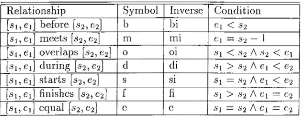
W e choose to use 8 directional and 8 topological relations whose definitions are based on A llen’s temporal interval relationships [3]. Table 3.1 lists A llen ’s temporal interval relationships, and Tables 3.2 and 3.3 list directional and topological relations and their definitions in terms of A llen’s temporal intervcd relationships, respectively. In Table 3.1, [¿j·, Ci] denotes an interval where s,; is the starting point and Cj is the ending point of that interval. In Tables 3.2 and 3.3,

Oi

i

[x\,.,X

]oi

X

]o

[

,X

]

M ^ U X

]

[

X

]

MA U ^

]

·

Relationship Symbol Inverse C o n d i t i o n

[si,ei] before [52,62] b bi 6i < 52 [si, ei] meets [52,62] m m i 61 = 5 2 - 1 [51, Cl] overlaps [52, 62] 0 o i 6*1 < 6‘2 A S2 <

¡51, ei] during [52,62] d di 5i > 52 A 6i < 62 [51,61] starts [52,62] s si Si = 6*2 A Cl < 62

[51, 6i] finishes [52,62] f fi 5i > 52 A 61 = 62 [51,61] equal [52,62] e e 5i = 52 A 6 i = 62

Table 3.1: Intervcil Relationships

Let

S

S -- [norths south, east, west, northeast, northwest, southeast, southwest, null}

and

T

CHAPTER 3. INDEX CREATION

17

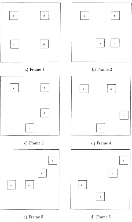
a) Frame 1 b) Fi'cime 2

c) Frame 3 d) Frame 4

c) Frame 5 d) Frame 6

CHAPTER 3. INDEX CREATION

₁₈

Relation

Definition

oi south 02 *1, X'ijoi {d ,d i,s,si,f,fi,e}[xi,

X

]o

o\

Ol (Ycist O

(¡0:1, o:'2]oi {o )[o :,, 0:2)02 A [2/1,2/2)01 {b ,m ) [2yi, 2/2)02)

0| south-ecist 02

_{([0:1,0:2)01 {bi,rni}[o:i,0:2)02 A[}

₂

_/

, 2/2)01 {b,m,o}[

2

/i,2/2)0,) V

(¡0:1,0:2)01 {oi}[a:i, 0:2)02 A [2/1,2/2)01 {b,m}[2/1, y2]02)

Oi north-west 02 ([a :i,*2)01 {b ,m }[o :i,0:2)02 A[2/i,2/2)01 {b i,m i,o i}['i/i,2/2)02) V (¡0:1, .o:2]oi {o}[o;i, ^2)02 A [2/1,2/2)01 {b i,m i)[2/i, 2/2)02)________ 6>| north-east 02 ([.г·ı,^2)01 {bi,mi}[.'Ci,.'1-2)02 A[2/i,2/2)01 {b i,m i,o i}[2/ i ,2/2)02) V

(¡0:1, .'r2]oi {oi}[x-i,.T2)o2 A [2/1,2/2)01 { b i,m i) [2/1,2/2)02) Table 3.2: Definition of Directioiicil Relations

Ccirtesian product of the sets

S

T

I

S'I\

ST = S x T - I

or

ST

{equal

null, inside

null, contain — null, cover — null, coveredby —

null, overlap—null, touch—north, touch—south, touch—east, touch—west, to u ch -

northwest, touch — northeast, touch — southioest, touch — southeast, disjoint —

north, d isjoin t—south, d isjoin t—east, d isjoin t—west, d isjoin t—northwest, disjoint-

northeast, disjoint — southwest, disjoint — southeast}

3.1.2

Spatial Partitioning

On the basis of the definitions given in the previous subsection, we provide the following formulation for spatio-temporal data on which SM IST-index is constructed.

CH APrER 3. INDEX CREATION

19

CHAPTER 3. INDEX CREATION

20

Relation

Definition

Oi equal 02

_{[a:i,^C2]oi{e}[3^i,3:2)02 A [y i,^2)01 { e }[y i,^2]}

Oi

oi

Oi

([3:1,3:2)01 {o,oi} [0:1,0:2)02

A [2/1,2/2)01 {d,di,s,si,f,fi,e,o,oi}[2/1,2/2)02) V

A [2/1,2/2)01 {o,oi}[2/1 >2/2)02) ____

o\

_{([3:1,3:2)01 {d i}[0:1,0:2)02 A [2/1,2/2)01 {fi,si,e}[2/ i,2/2)02) V}

([a:i,0:2)01 {e }[0:1,0:2)02 A [2/1,2/2)01 {di,fi,si}[2/1,2/2)02) V

(¡3:1, ■ ^2)oi{fi,si}[0:1,0:2)02 A [2/1,2/2)01 {di,fi,si,e}[2/1,272)02)

(¡3^’ i ,3:2)01 { e }[3: i ,0:2)02 A [t/i,2/2)01 {d ,F ,s}[2/1,2/2)02) V ( [3:1,3:2)01 { f,s } [o :i,0:2)02 A [2/1,2/2)01 { d ,f,s ,e } [2/1,2/2)02) Oi touch 02

([3:1,3:2)01 {m ,m i}[0:1,0:2)02 A

[171,2/2)01 {d,di,s,si,f,fi,o,oi,m,rni,e}[2/1,2/2)02) V

([3:1,3:2)01 {d,di,s,si,f,fi,o,oi,in,mi,e}[:i:i, 0:2)02

A [7/1,2/2)01 {m ,m i)[2/1,2/2)02)______

___

oi disjoint 02

[3:1,3:2)01 {b ,b i}[3:1,0:2)02 V [7/1,2/2)01 {b,bi}[?7i, 2/2)

Definition

spatio-temporal relation

•

Oi

•

tcli

(tdi

ST),

• s

e

Figure 3.2 shows the

spatio-temporal relations

x ,y

x

y,

b)

a

b

b

spatio-temporal relation

CHAPTER 3. INDEX CREATION

21

Relation Type

Spatio-Temporal Relation Set

{(a ,6 ,d -w ,l,4 ),(c ,d ,d -w ,l,2 ),(a ,c ,d -w ,5 ,5 )} {(6 ,g ,d -e ,l ,4 ),(d ,c ,d -e ,l,2 ),(c ,g ,d -e ,5 ,5 )} {(g ,(/,d -n w ,l,4 ),(g ,c ,d -n w ,2 ,4 ),(6 ,d ,d -n w ,4 ,4 ), (g ,c ,d -n w ,6 ,6)} {(f/,g ,d -s e ,l,4 ),(c ,g ,d -s e ,2 ,4 ),(d ,6 ,d -s e ,4 ,4 ), (c ,g ,d -se,6 ,6)} { ( g ,c ,d -n ,l,l) ,( 6 ,d ,d -n ,l,3 ) } { ( c ,g ,d -s ,l,l) ,( d ,6 ,d -s ,l,3 ) } {(6 ,c ,d -n e ,l,6 ),(6 ,g ,d -n e ,5 ,6 ),((/,g ,d -n e ,5 ,6 ), (d,c,d-n e,3,6),(6,(:/,d-n e,5,6)} { (c ,6,d - s w ,l,6) ,( g ,6,d -sw ,5,6),(g,f/,d -sw ,5,6), (c,d ,d -sw ,3,6),(d ,6,d -sw ,5,6)}

Table 3.4:

SMIST-'index

S M IT S constructs a tcible, whose size is equal to the Ccirdinality of

S7'

S I )

spatio-temporal relation

spatio-temporal relations

3.2

Temporal Organization

A t the second step of the construction of

SMIST-'mdex,

MIS-tvee

MIS-tvee

CHAPTER 3. INDEX CREATION

A l g o r i t h m

ProduceCommonTimeIntervals{R)

R

spatio-temporal relations

1

merge

L

set

L

max

3

set

L

min

for

m = min

max

do

5

produce

maximal set

common time interval

for

spatio-temporal relation (oi,Oj,tdk.,s,e)

R

do

7

for

m,aximal set M

do

8 i f [.s, e] intersects

common time interval

add (oi,O j,td k,s,e)

10

so7't

maximal sets

common time intervals

set M

maximal set

12

while

M

maximal set

do

13 i f M = n e x t

maximal set

14

set

common time intei'val

M

common time interval

maximal set

15

remove

maximal set

set M

maximal set

Figure 3.3: The algorithm for production of

maximal sets

[sO, Co], [iii, Cl], ..

which will be Ccilled

common time intervals,

maximal set

spatio-temporal relations,

(0 < z <

n)

Definition

maximal set M ,

common time intei'val < Sc,Cc > ,

spatio-temporal

'elations

1. For each

spatio-temporal relation d <

i ,

,td i,s,.e >

M ,

Sc

tc-2. For each

spatio-temporal relation d <

i ,

,td i,s ,e > , s < Sc

d e M .

Given the

spatio-temporal relations d i,d

, ...,dm, common time intervals

maximal sets Ado, M \,..., M,^

CHAPTER 3. INDEX CREATION

23

(a,b,d-w,l,4)

(c,d,d-w,l,2)

(a,c,d-w,5,5)

Figure 3.4: T im e intervals of

Spatio-temporal relations

Figure 3.4 through 3.7 show time intervals of rehitions for each topological- directiomil relation type that exists in the example data of Figure 3.1, and Table 3.-5 through 3.8 show

maximal sets

maximal sets

M axim al Set Com m on Tim e Intervcil

Mo - {

Ml

M'z

Table 3..5: M axim al sets and corresponding common time intervals for disjoint- west

Theorem,

S

maximal sets. Common time intervals

n

maximal sets

CHAPTER 3. INDEX CREATION

24

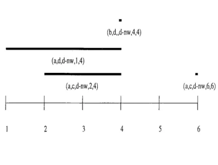
(b,d„d-nw,4,4)

(a,d,d-nw,l,

4

)

(a,c,d-nw,2,4)

(a,c,d-nw,6,6)

Figure 3.5; T im e intervals of

Spatio-temporal relations

(a,c,d-n,l,l)

i,d,d-n ,l,3)

2 3 5 6

CHAPTER 3. INDEX CREATION

25

Figure 3.7: T im e intervals of

Spatio-temporal relations

M axim al Set Com m on T im e Interval

M\

M

Table 3.6: M axim al sets and corresponding common time intervals for disjoint- north

Co < A Cl < ¿'2 A ... A < Cji

liolds.

P roof 3.1

L

common time intervals

ProduceCommonTimeIntervals

L

ench

si =

n).

spatio-temporal relations

‘maximal sets.,

maximal sets

com-rnon time intervah.

common time interval

common time interval

maximal

comm,on time interval

ci+\]

CHAPTER 3. INDEX CREATION

26

Mcixirnal Set Com m on T im e Interval

Mo

Ml

Nh

Ms

Table 3.7: M axim al sets and corresponding common time intervcils for disjoint- northwest

M axim al Set Com m on 'Time Interval

Mo

Ml

M

(c/,a ,d -n e,5,6),(6,(/,d -n e,5,6)}

[5,6]

Tcible 3.8: M axim al sets and corresponding common time intervals for disjoint- northeast

is deleted. Since e/+i < the total order between the

common time intervals

After producing all the

maximal sets,

SMIST-index

Chapter 4

Query Execution

As we have stated before, queries of concern in this work ¿ire the ones that involve motion of multiple objects which is specihed by the change in o b jects’ relative sj^aticil positions. Therefore, a query consists of specification of rehitive positions of objects in a sequence of frames. This kind of ci. query is different from the one in which the trajectory of each object is explicitly defined. Thus, spcitial relationships between objects gain special importance for the queries of our concern. Another important property of such queries is tlicit identities of the objects are not specified. Therefore, to answer a query we have, to find a similar spcitial structure that is a set of objects whose spatial relations between each other is the same as that in the first frame in the query. Then, in order to decide whether it is actually the answer, consequent frames should be compared with that of the query.

The expensive part of execution of such a query is matching the first frame of the query with some frames in the database. Once a matching frame is found and object identities are specified, checking whether the o b jects’ spatial structure in the following frames is similar to the one defined in the query is straightforward. Therefore, we focus our attention on finding a similar frame for the first frame of the motion query.

Definition

structural query Q