0885–3010 © 2014 IEEE
abdullah atalar, Fellow, IEEE, Hayrettin Köymen, Senior Member, IEEE, and H. Kağan oğuz, Student Member, IEEE
Abstract—Using the small-signal electrical equivalent circuit
of a capacitive micromachined ultrasonic transducer (CMUT) cell, along with the self and mutual radiation impedances of such cells, we present a computationally efficient method to predict the frequency response of a large CMUT element or array. The simulations show spurious resonances, which may degrade the performance of the array. We show that these un-wanted resonances are due to dispersive Rayleigh–Bloch waves excited on the CMUT surface–liquid interface. We derive the dispersion relation of these waves for the purpose of predicting the resonance frequencies. The waves form standing waves at frequencies where the reflections from the edges of the element or the array result in a Fabry-Pérot resonator. High-order res-onances are eliminated by a small loss in the individual cells, but low-order resonances remain even in the presence of sig-nificant loss. These resonances are reduced to tolerable levels when CMUT cells are built from larger and thicker plates at the expense of reduced bandwidth.
I. Introduction
c
apacitive micromachined ultrasonic transducers (cmUTs) are wideband transducers [1] with very low loss. because individual cmUT cells are small, in practice many of them are connected in parallel to form larger transducers. crosstalk between the cells of an array has been of considerable interest [2]. The artifacts observed in the point spread function of cmUT arrays were attrib-uted to crosstalk between the elements [3]. The spurious responses were believed to be due either to stoneley waves [4] in the interface or to lamb waves [5] in the substrate. scholte [6] waves traveling in the interface between the array surface and the immersion medium were also held responsible. Using finite element models and optical dis-placement measurements, acoustic coupling through the fluid medium was found to be the major source of cross-coupling between the elements [2]. dummy elements on the substrate or reflections from the edges of the substrate also introduced unwanted responses [4].Eccardt et al. [7] described a dispersive surface wave on cmUT arrays by considering infinitesimally small cmUT cells. They derived an analytical expression that defines the phase velocity of the surface waves as a function of fre-quency. analysis of infinitely large cmUT arrays was car-ried out using an impedance matrix and the Fourier trans-form method [8]. The results indicated the presence of
parasitic surface waves, which may be damped by resistors in series with each cmUT cell. a spectral finite element analysis/boundary element method was used to predict the response of infinite quasi-periodic cmUT structures for the purpose of finding dispersion characteristics of pos-sible parasitic waves like leaky rayleigh, stoneley–scholte, and lamb waves [9]. The method predicted the presence of a slow dispersive wave at low frequencies caused by cross-talk between the cells with a cut-off frequency deter-mined by cell pitch. This spurious surface wave was used as a sensor of fluid viscosity [10].
The acoustic mutual coupling between the cells and the response of a single cell were combined in a small-signal model to simulate the response of five cmUT cells using a piston radiator assumption, indicating an uneven response [11]. a small-signal analytical method covering a selected number of higher order plate modes was implemented to predict the response of a group of cmUTs [12]. The num-ber of unknowns is equal to the numnum-ber of cells multi-plied by the number of cmUT plate modes. The mutual impedance between the cells was calculated numerically from the rayleigh integral. limited by the computation time, the mutual impedance was ignored beyond a rela-tively small radius. The method was able to predict cou-pling between different plate modes in a seven-cell cmUT configuration. The response of a cmUT array containing 1280 cells was also computed, indicating sharp peaks in the low-frequency response [13].
In this paper, we first present a computationally effi-cient method to simulate large cmUT elements or arrays containing thousands of cells. We employ a small-signal equivalent circuit of an individual cell modeling only the lowest order mode of the cmUT plate, hence the number of unknowns is equal to just the number of cells. The mutual radiation impedances in the immersion medium between all cells are included using an analytical approxi-mation. our method is accurate at low frequencies when the coupling between the cells is strong, but it does not predict the response at high frequencies where the high-er ordhigh-er modes are excited. We show that the spurious resonances observed at low frequencies are due to ray-leigh–bloch waves excited on the surface of the elements or arrays.
II. single cmUT cell in Immersion
let us consider a circular full-electrode single cmUT cell as shown in Fig. 1.
The immersed cmUT can be represented by an electri-cal equivalent circuit [14] as shown in Fig. 2. This simple manuscript received July 1, 2014; accepted september 29, 2014.
a. atalar and H. Köymen are with the department of Electrical and Electronics Engineering, bilkent University, ankara, Turkey (e-mail: [email protected]).
H. K. oğuz is with the department of Electrical Engineering, stanford University, stanford, ca.
linear circuit only models the lowest order vibrational mode of the cmUT plate under small-signal regime; it does not predict the response at higher frequencies where higher order modes may be excited or for large signals where harmonics will be generated. The parameters of the circuit model are defined in the appendix for complete-ness. a series resistor, Ra, is inserted in the mechanical side to take care of the mechanical loss.
III. response of an array of N cells
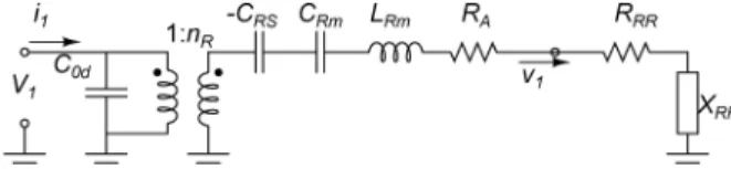
consider an array of m elements, each containing n identical cmUT cells, with a total of N = mn cells that are arbitrarily placed in a flat rigid baffle and are im-mersed in liquid. referring to Fig. 3, the mechanical ports of the cells are connected to an N-port represented by the Z matrix, which accounts for the self and mutual radia-tion impedances of the cells.1 For generality, the electrical port of each cmUT cell contains a series resistor, Rs. The array elements are connected to the voltage sources repre-sented by the phasors, Vin1, Vin2, …, Vinm, all with source impedances of RT.
To solve the cell velocities, vp, for p = 1, 2, …, N, we write n Vp j L m j C C R Z ka v m p q R R R RS A RR = 1 1 1 ( ) = ω + ω − + + + 11 ( , ) q p N pq q Z ka kd v ≠
∑
M . (1) This set of N equations can be written in matrix form asnRV = ( )M vω , (2)
where V and v are column vectors of the voltages, Vp, and the velocities, vp, for p = 1, 2, …, N, respectively. M(ω) is an N × N square matrix with the entries defined as in (1). With i being defined as an N × 1 column vector of cur-rents i1, i2, …, iN, we write
i = j Cω 0dV+nRv. (3)
If VE is an N × 1 column vector of element voltages with appropriate entries equal to VE1, VE2, …, or VEm, we have
VE = RSi+ .V (4)
Finally, we express Vin, an N × 1 column vector of drive
voltages with corresponding entries equal to Vin1, Vin2, …, or Vinm, as
Vin = RTJi+VE, (5)
where J is an N × N matrix, which contains m all-ones matrices (n × n each) along its diagonal to add the cur-rents of the cells appropriately. combining the matrix equations (2)–(5), we reach
nRVin = ( )Ψ ωv with (6)
Ψ( ) = [ω j C Rω 0d( TJ+RSI)+I M] +n RR2( TJ+RSI), (7) where the I is an N × N identity matrix. Hence, the cell velocities, v, can be found at ω by the inversion of the N × N Ψ(ω) matrix. For an 80 × 240 array with 48 elements (m = 48, n = 400), the Ψ matrix of 19 200 × 19 200 needs to be inverted. If a symmetry exists, the size of the matrix can be reduced.
once the velocities of the individual cells, v, have been found, the input currents of elements, iin1, iin2, …, iinm, defined by iin column vector can be determined from (2)
and (3): iin = J j Cωn 0dM( )ω nRI R + v. (8)
Fig. 1. cross-sectional view of a cmUT cell of radius a with full elec-trode.
Fig. 3. small-signal equivalent circuit of an array of cmUT cells im-mersed in a liquid medium. Elements are driven by ac voltage sources, Vin1,…,Vinm, each with a source resistance RT. a resistor, Rs, is placed
in series with each cell.
1 Z is a full matrix because the mutual radiation impedance function is
Hence, the absolute acoustic power output, Pout, delivered to the liquid medium can be found as the power input minus the power dissipated on resistors Ra, RT, and Rs as follows: P V i R v R i R p m p p p N p p m p out in in A T in Re =12 { } 12 1 2 12 =1 * =1 2 =1 2
∑
∑
∑
− − − SS p N p i =1 2∑
. (9)We developed a matlab (The mathWorks Inc., natick, ma) code utilizing array operations to make use of multi-core processors. The code is optimized so that matrix in-version determines the execution time, while the matrix-fill time is a small fraction. It is verified with the results of our earlier simulations [15] which used a harmonic balance simulator. In all simulations that follow, the cell dimen-sions are adjusted so that they have a collapse voltage of Vc = 55 V under 1 atm = 101.3 kPa pressure and a single-cell resonance frequency of 1.4 mHz in water. The elements are driven by a sinusoidal unit voltage source of
RT = 50 Ω resistance with Rs = 0, and cmUT cells are biased with Vdc = 50 V.2
A. Single-Array Element Simulations
The cells of dimensions a = 30 μm, tm = 0.94 μm, and
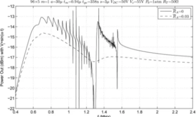
tge = 358 nm are placed in a rectangular grid of 96 × 5 in a single element with a cell-to-cell separation of s = 3 μm. Initially, the mechanical loss resistor, Ra, is assumed to be zero. The solid curve in Fig. 4 shows the acoustic pow-er output calculated from (9) as a function of frequency. note the presence of spurious resonances for frequencies lower than 1.6 mHz.
losses present in the cmUT cells can cause the spuri-ous resonances to disappear [8]. The loss can be intro-duced by adding a series resistor to each cell [16] (Rs) or by adding a lossy layer on top of the cmUT cells [17] at the mechanical side. The effect of the mechanical loss can be investigated by using a nonzero value for Ra.3 The dashed curve in Fig. 4 presents the calculated power out-put of the same element, with RA = Ra/ρ0c0πa2 = 0.03
resulting in about 0.6 db reduction in the output power. The calculated curves are similar to experimentally mea-sured responses of arrays [4], [18], [19]. This damping gets rid of the high-Q resonances, but remnants of some reso-nances are still there.
We note that it is relatively difficult to introduce a loss in the electrical side. because the individual cmUTs have high electrical impedance, a series resistor (Rs) for each cell on the order of 100 kΩ is necessary to introduce a significant loss.
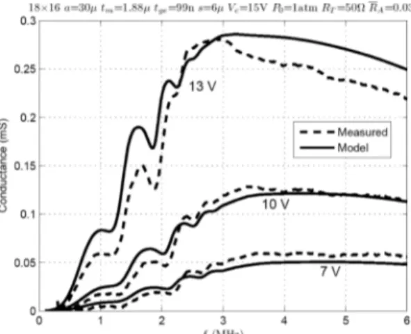
Fig. 5 shows the layout of a cmUT element with 18 × 16 hexagonally packed cells. The devices were fabri-cated [20] with a low-temperature surface micromachin-ing technology utilizmicromachin-ing a cr sacrificial layer and si3n4 deposition by a plasma-enhanced chemical vapor deposi-tion system. The electrical impedance measurements are carried out using a 50-Ω network analyzer. Fig. 6 depicts a comparison of calculated and measured conductances4 of the element under different bias voltages. The spurious resonance frequencies are predicted very well, verifying the validity of the model.
B. Array Simulations
We simulate a 1-d linear array with 48 elements made up of cells with a = 36.3 μm.5 Each element contains 80 × 5 rectangularly placed cells with a separation of s = 3 μm. Elements are driven at 0.70 mHz by linearly in-creasing delays of 0, 1/8, 2/8, …, 47/8 μs (Δ = 1/8 μs) to simulate a case where the beam is steered at an angle Fig. 4. acoustic power delivered by a single array element (m = 1, N =
n = 96 × 5 = 480) of size (defined in water at 2 mHz) as a function of frequency. The cells have a radius of 30 μm with no loss (RA = 0, solid
line) and with a 0.6 db loss (RA = 0.03, dashed line) are placed in a
rectangular pattern.
Fig. 5. layout of a cmUT element with hexagonally packed 18 × 16 cells. The cells have si3n4 plates with dimensions a = 30 μm, s = 6 μm,
tm = 1.88 μm, tg = 70 nm, ti = 160 nm, and material constants are Y0 =
140 GPa, ρ = 3100 kg/m3, σ = 0.27, εr = 5.4.
2 We use Y0 = 320 GPa, σ = 0.263, ρ = 3270 kg/m3, c0 = 1500 m/s,
and ρ0 = 1000 kg/m3, unless noted otherwise. available power from the
source is 4 dbm.
3 The resistor Ra may well have a frequency dependence, but we
as-sume it to be independent of frequency.
4 a square-law frequency-dependent conductance due to the loss in
the insulator layer at zero bias is subtracted from the measured conduc-tances.
5 tm = 1.31 μm, tge = 325 nm to satisfy Vc = 55 V and a single cell
of θ = 30° with respect to the normal. The calculated cell velocity distribution is shown in Fig. 7 as a grayscale map demonstrating uneven velocities within the elements and the array. The electrical conductances of the elements are also shown in the same figure, indicating a large variation between the elements.
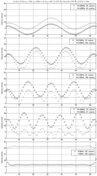
next, we simulate another 1-d linear array with sixty-four elements made up of cells with 26% larger cells: a = 45.7 μm.6
The elements are driven by equal voltages with linearly increasing delays: 0, 1/8, 2/8, …, 63/8 μs (Δ = 1/8 μs). The velocity magnitudes of individual cells obtained from (6) with RA = 0.03 are shown in Fig. 8 at different
fre-quencies showing a considerable nonuniformity in cell ve-locities.7 Fig. 9 shows the plots of the velocity distribution along selected columns of the same array at the same fre-quencies, quantitatively depicting the uneven velocity dis-tribution. note that the nature of nonuniformity is differ-ent at 2 mHz, where the velocity fluctuation is minimal within a column, but substantial among different columns of the same element.
IV. normalized Velocity Fluctuation To compactly quantify the amount of fluctuation in the velocities, we define a normalized velocity fluctuation, v, within the array using the absolute value of the deviation from the average velocity as a function of frequency:
v v f N p v f v f N p ( ) = 1 ( ) ( ) =1 max
∑
− , (10)Fig. 6. calculated (solid) and measured (dashed) conductances of the 18 × 16 element immersed in sunflower oil with bias voltages of Vdc = 7,
10, and 13 V. The constants of vegetable oil are c0 = 1450 m/s and ρ0 =
915 kg/m3. The loss resistance of cmUTs is selected as R
A = 0.035 for
a good fit.
Fig. 7. Upper graph: calculated velocity magnitude map of an array of 80 × 240 cells divided to 48 elements (each element is about 2.8λ × 0.17λ with λ defined in water) at 0.70 mHz. lower graph: conductance of elements. The cells have a radius of 36.3 μm with 0.6 db loss and are placed in a rectangular pattern. Elements are excited with increasing delays (Δ = 1/8 μs).
Fig. 8. calculated cmUT velocity magnitude distribution of a 64 × 256 array (N = 16 384) with sixty-four elements (m = 64) made up of rectangularly packed cells with radius a = 45.7 μm with 0.6 db loss at 0.46, 0.62, 0.72, 0.84, and 2.00 mHz. vm is the maximum velocity in each
graph. Elements of 64 × 4 cells are approximately 8λ × λ/2 in size, where λ is defined in water at 2 mHz and they are excited with increas-ing delays to steer the beam at θ = 30° with respect to the normal (Δ = 1/8 μs).
6 tm = 1.92 μm, tge = 298 nm to maintain the same Vc and the same
resonance frequency.
7 computation time for the array of 64 × 256 cells (N = 16 384) is 350
s per frequency point on an Intel i7-4800mq cPU (Intel corp., santa clara, ca) running at 2.7 GHz clock.
where v f( ) is the average velocity amplitude within the array of N cells at frequency f, and normalization factor
v max is the average velocity at the center frequency. v = 0 means that all cells move with the equal amplitude with-in the array, whereas a nonzero value of v imply a varia-tion in the velocities of cells within the array. Fig. 10 shows calculated values of v of the array of section III-b as a function of frequency. The spurious resonances are seen as peaks in the graph. The same graph also shows v while the acoustic loss is increased. a higher acoustic loss reduces the fluctuation as expected. Fig. 11 is a similar graph when the delays between the excitations of neigh-boring elements are varied. as the delay, Δ, is increased (resulting in a higher steering angle, θ), the fluctuation increases, especially at frequencies higher than the reso-nant frequency of the single cell. The lowest fluctuation occurs when all elements are excited with the same volt-age.
To see the effect of cmUT cell parameters on the v performance, we simulated two more arrays with larger
and thicker plates with the same resonance frequency (1.4 mHz) and collapse voltage (55 V). The first one has medium-size cmUT cells: a = 94.2 μm, tm = 6.4 μm, tge = 227 nm. The radius of the cells is about two times larg-er, hence an array with the same area is obtained with 32 × 128 cells. Each of the 64 elements contains 32 × 2 cells. Fig. 12 depicts the performance of the array as a function of frequency for different delays between consecutive array elements. The fluctuation is somewhat reduced, but it is still relatively high. The second array (16 × 64) contains even larger cmUT cells with a = 189.9 μm, tm = 23.9 μm,
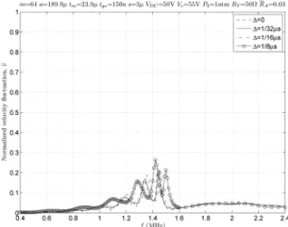
tge = 150 nm, where the elements are made from 16 × 1 cells. Fig. 13 shows v for this array of the same overall size. as the cmUT cells are made larger, v is considerably reduced. For comparison, the acoustic power outputs of the three arrays are plotted in Fig. 14 as a function of frequency. note that the power output of the array with largest cells is 11 db higher than that with the smallest cells at the center frequency because of a better imped-ance match at the expense of reduced bandwidth.
Fig. 9. calculated cmUT cell velocity magnitude distribution along se-lected columns of the 64 × 256 array of Fig. 8 at 0.46, 0.62, 0.72, 0.84, and 2.00 mHz.
Fig. 10. calculated normalized velocity fluctuation ( )v within the array of Fig. 8 as a function of frequency for various acoustic loss levels of 0.3, 0.6, and 1.7 db (RA = 0.015, 0.03, 0.09). v max is defined at 2 mHz.
Fig. 11. calculated normalized velocity fluctuation ( )v within the array of Fig. 8 as a function of frequency for various delays between neighboring cells, corresponding to 0°, 7°, 14°, and 30° steering angles.
V. dispersive rayleigh–bloch Waves
It is known that periodically placed resonators support surface waves known as rayleigh–bloch (r-b) waves [21]. linton and mcIver [22] showed that these waves can exist along the surface of periodic structures in the absence of any incident waves. It was pointed out that r-b waves can exist on the cmUT–fluid interface [8]. These waves exist along the periodic structure surface with no leakage into the surrounding medium, because their phase velocity is slower than that of a bulk wave in the liquid medium. The dispersive surface wave detected on the surface of infinite cmUT structures [9] is the r-b wave.
To find the characteristics of the possible r-b waves, we follow the approach of collin [23] and consider an in-finite element of cmUT cells with no mechanical loss. as an example, we consider two infinite rows of cmUT cells as shown in Fig. 15, all driven in parallel with an ac voltage source of Vin (with RT = 0). let d represent the distance between the centers of the neighboring cells.
We assume that an r-b wave exists, propagating in the
x-direction with a phase velocity of vb. (It is not possible to support an r-b wave in the y-direction because of sym-metry.) We represent this interface wave by e− (jω/v xB).
be-cause of the infinite geometry, the surface wave amplitude must have no x dependence. Therefore, all cells must vi-brate with the same plate velocity, v1, except for the phase factor given by e− (jω/v xB), where x is the position of the cell
center. For any cell, we can write the following equation, which includes the mechanical and self-radiation imped-ance of the cell as well as the mutual impedimped-ance of all the other cells: n VR in = ( )Ψ ωv1 (11) Ψ( ) = 1 ( ) ( , ) =1 ω ω ω j L j CC CC Z ka Z ka kd e m m m q N R RS R R RS RR M + − +
{
+ + →∞ −∑
( jj v qd ej v qd Z ka kdq Z ka kd q ( ) ( ) ) . ω/ ω/ M M B + B [ ⋅(
( , )+ ( , 2 +1))]
}
(12) The exponential factors in the infinite summation of Ψ account for the phase differences of the neighboring cells with x-separation of qd on the left and on the right. The factor d q2 +1 defines the distance between the centersof the cells in the alternate rows. For a given ω, v1 will be maximized if Ψ is minimum. This condition is met if the imaginary part of Ψ is zero. To find vp in terms of ω, we can write this condition as the dispersion relation:
Im{ ( )} = 0Ψ ω . (13)
Fig. 12. calculated normalized velocity fluctuation ( )v within a same size 32 × 128 array built from medium size cells as a function of frequency for various delays between neighboring cells.
Fig. 13. calculated normalized velocity fluctuation ( )v within a same size 16 × 64 array built from large size cells as a function of frequency for various delays between neighboring cells.
Fig. 14. calculated acoustic power outputs of the three arrays of the same overall size as a function of frequency. The total available power from the electrical side is 22 dbm, indicating a center-frequency conver-sion loss of 17.5, 13, and 6.5 db, respectively.
Fig. 15. Geometry of two infinite rows of cmUT cells. dashed lines show the distances to neighboring cells for q = 2 in (12): 2d and d 22+ .1
For the purpose of numerical evaluation, the upper limit of the infinite summation in (12) is taken as N such that
Nd > 40λ = 40ω/c0 (with λ defined at the frequency of single cell resonance). In Fig. 16(a), we plot the dispersion curve for the cmUT element of Fig. 15, composed of cells with a = 30 μm, tm = 0.94 μm, s = 3 μm, and a single-cell resonance in water of 1.4 mHz. because of symmetry, the dispersion relation is also valid for a surface wave traveling in the opposite direction (e+ ω/j( v xB)) with the same phase velocity.
The dispersion relation of r-b waves given by (12) and (13) is valid for the infinite element with two rows shown in Fig. 15, where all cells have the same amplitude. If the actual element length is not infinite, but sufficiently long, the dispersion relation is nearly the same. However, if the number of rows is different or if the element size is very small, the relation is modified.8
If the element is of finite length, the reflections of r-b waves at the edges can create Fabry–Pérot type standing waves at distinct frequencies when the element length is an integer multiple of the wavelength. only even sym-metric standing waves, shown in Fig. 9, are possible. odd symmetric standing waves are not excited, because all cmUT cells within the element are driven equally. For an element of length D, the standing wave condition can be expressed as
D =pλ=pvfB, with p= 1,2,…. (14)
In Fig. 16(a), we also plot (14) as straight lines for p = 3, 4, …, 18 and D = 2709 μm. The intersections of the straight lines with the dispersion curve give the approxi-mate resonance frequencies of the element. Fig. 16(b) is a plot of the normalized velocity fluctuation of this 2 × 44 element near the spurious resonance frequencies. a com-parison of Figs. 16(a) and 16(b) shows that the resonance frequencies are correctly estimated from the dispersion curve graph.
The Fabry–Pérot resonances of the array of Fig. 8 are clearly seen as standing waves in Fig. 9 and peaks in the graph of Fig. 10. notice that a lower but significant v ex-ists even at frequencies higher than the cut-off frequency of r-b waves. Uneven loading of cmUT cells within an element, especially for the cells near the periphery of the
element or when the neighboring elements are excited with different excitation voltages, is the reason for the nonuniformity.
The resonance frequencies can be found more accurate-ly for a finite-size element or array by using (6). To maxi-mize the velocities, v, the magnitude of the determinant of Ψ must be minimal. This occurs at frequencies where the imaginary part of the determinant of Ψ is zero:
Im{ ( ( ))} = 0det Ψ ω . (15) Using this method, the resonance frequencies are calcu-lated and listed in Table I. The values agree well with Fig. 16(b).
The quality factor, Q, at a resonance, ω0, can be es-timated from the quality factor of the determinant of Ψ around ω0:
Fig. 16. (a) dispersion curve (thick curve) for r-b waves on two infinite rows of cmUTs (Fig. 15) immersed in water. standing wave condition of (14) is also plotted for p = 3, 4, …, 18 and D = 2709 μm (thin lines). (b) normalized velocity fluctuation of the 2 × 44 cmUT element with a = 30 μm, tm = 0.94 μm, s = 3 μm, D = 2709 μm, RT = 0, Ra = 0,
and Rs = 0.
f0 (mHz) 1.473 1.498 1.520 1.539 1.555 1.569 1.580
Q 2540 1169 830 621 479 432 393
8 a rearrangement of cmUT cells within the element or placement of
different-sized cmUT cells in the element do not eliminate r-b waves. such approaches simply cause a change in the dispersion curve and a shift in the spurious resonance frequencies.
mechanical resonance of a single cell in water. Q drops as the frequency changes in both directions.
The dispersion curve indicates that there is a cutoff frequency (1.6 mHz in the examples) above which no r-b wave can exist. The presence of such a cutoff frequency was reported earlier from simulations [9] and experimen-tal data [24]. our simulations show that above 1.6 mHz, although there is a nonuniformity in the cell velocities, no standing-waves exist. This cutoff frequency was not pre-dicted by the dispersion curve of surface waves assuming infinitesimally small cmUTs [7]. The cutoff arises from the bragg condition when the cmUT cell pitch is equal to a half wavelength of the r-b wave. We note that the dispersion curve shown in Fig. 16(a) is only representative because it depends on the cmUT dimensions, the separa-tion between the cells, etc. different cmUT geometries give rise to different dispersion curves.
our circuit theory model cannot predict the excitation of stoneley, scholte, or lamb waves. It is plausible that these waves may be excited at the discontinuities of the element, such as its edges.
VI. conclusions
We are able to simulate large arrays of cmUT cells using the small-signal equivalent circuit in a computation-ally efficient manner. The simulation results agree well with the experimental measurements. The spurious reso-nances seen around the resonance frequency of a single cell can be attributed to r-b waves present on the interface between the cmUTs and the immersion medium. They are created by the mutual interactions between the cells through the mutual radiation impedance. The resulting r-b waves are highly dispersive and have a phase velocity less than the speed of sound in the immersion medium. The spurious resonances occur when an element or array dimension is an integer multiple of the r-b wavelength. at these frequencies, there is a significant cell velocity fluctuation within an element. The inherent loss of real cmUT elements, such as the loss in the polymer protec-tion layer, can be sufficient to eliminate some resonances. The high-order spurious resonances disappear if there is about 0.6 db loss in the transducer, whereas the low-order resonances remain even in the presence of a significant loss factor. There is a cut-off frequency above which no r-b wave can exist. However, velocity fluctuations exist even above the cut-off frequency because of nonuniform loading of the cells, especially when the neighboring ele-ments are excited with different voltages. If arrays are built from larger and thicker cmUT cells, the velocity variation caused by r-b waves and nonuniform loading of
A. Small-Signal RMS Equivalent Circuit of a CMUT Cell
referring to Fig. 1, the circular cmUT cell has a radius of a, a plate thickness of tm, and an effective gap height of
tge = tg + ti/εr, where εr is the relative permittivity of the insulator material. The component values of the small-signal rms equivalent circuit of Fig. 2 can be expressed as [14] u = t5XR t =t ti r ge with ge g+ /ε (17) C0d =C g u0 ( ) with C0 = 0t a2 ge ε π (18) nR C g u Vt DC L m a tm ge R = 5 0 ′( ) , =ρπ 2 (19) C t C V g u C a Y t m m RS ge DC R = 2 5 ( ) = 9 5(116 ) 2 0 2 2 2 0 3 ′′ − , σ π (20) V V ug u F F DC r Rb Rg = 3
(
2 ( )−′)
(21) V t a t Y m r / ge/ = 8 27 (1 ) 3 2 2 3 2 0 0 2 ε −σ (22) F t C m F a P Rg ge R Rb = 5 = 5 3 2 0 , π (23) V Vcr ≈ − FFRbRg + FFRbRg− + 0.9961 1.0468 0.06972 0.25 0. 2 001148 FFRb 6 Rg (24) g u( ) = tanh−u1 u, g u′( ) = 21u1−1u−g u( ) (25) g u u u g u ′′ ′ − − ( ) = 21 1 (1 )2 3 ( ) . (26)Xr is the static rms displacement of the plate under a bias voltage of Vdc and a static pressure of P0. Vr and Vc are the collapse voltages under vacuum and under pressure
P0. Y0, σ, and ρ are, respectively, the young’s modulus, Poisson ratio, and density of the plate material. ε0 is the permittivity of free space.
B. Self- and Mutual Radiation Impedances of Circular CMUT Cells
consider an immersion liquid of density ρ0 and sound velocity c0. For the rms equivalent circuit, the normalized
tion impedance of a piston transducer of radius a at very high frequencies. We have
R ka R c a ka F ka RR( ) = RR 1 5 2 (2 ) (2 ) 0 0 2 11 7 122 ρ π ≈ − (27) X ka X c a ka F ka RR( ) = RR 5 2 (2 ) (2 ) 0 0 2 11 7 222 ρ π ≈ − (28)
for 0.1 < ka < 3 with k = ω/c0 and
F y122 y J y2 5 yJ y4 J y3 y y 3 5 ( ) = ( )+2 ( )+3 ( )−16−768 (29) F y222 y H y2 yH y H y y y 5 4 3 4 6 ( ) =− ( ) 2− ( ) 3 ( )− +235+ 2945 π π , (30) where y = 2ka.
The mutual radiation impedance, Zm, between the two cells can be approximately written as [15]
Z ka kdM( , )≈ρ π0 0c a A ka2 ( )sinkd( )kd +jcoskd( )kd , (31)
where d is the distance between the centers of the cmUT cells and A ka p ka n n n ( ) = =0 10
∑
( ) , (32)with coefficient pi values given in [15, Table II]. references
[1] I. ladabaum, X. Jin, H. T. soh, a. atalar, and b. T. Khuri-yakub, “surface micromachined capacitive ultrasonic transducers,” IEEE Trans. Ultrason. Ferroelectr. Freq. Control, vol. 45, no. 3, pp. 678– 690, 1998.
[2] a. caronti, a. savoia, G. caliano, and m. Pappalardo, “acoustic coupling in capacitive microfabricated ultrasonic transducers: mod-eling and experiments,” IEEE Trans. Ultrason. Ferroelectr. Freq. Control, vol. 52, no. 12, pp. 2220–2234, 2005.
[3] o. oralkan, a. s. Ergun, J. a. Johnson, m. Karaman, U. demirci, K. Kaviani, T. H. lee, and b. T. Khuri-yakub, “capacitive micro-machined ultrasonic transducers: next-generation arrays for acous-tic imaging?” IEEE Trans. Ultrason. Ferroelectr. Freq. Control, vol. 49, no. 11, pp. 1596–1610, 2002.
[4] X. Jin, o. oralkan, F. l. degertekin, and b. T. Khuri-yakub, “characterization of one-dimensional capacitive micromachined ul-trasonic immersion transducer arrays,” IEEE Trans. Ultrason. Fer-roelectr. Freq. Control, vol. 48, no. 3, pp. 750–760, 2001.
[5] m. H. badi, G. G. yaralioglu, a. s. Ergun, s. T. Hansen, E. J. Wong, and b. T. Khuri-yakub, “capacitive micromachined ultra-sonic lamb wave transducers using rectangular membranes,” IEEE Trans. Ultrason. Ferroelectr. Freq. Control, vol. 50, no. 9, pp. 1191– 1203, 2003.
[6] J. mclean and F. l. degertekin, “directional scholte wave gen-eration and detection using interdigital capacitive micromachined ultrasonic transducers,” IEEE Trans. Ultrason. Ferroelectr. Freq. Control, vol. 51, no. 6, pp. 756–764, 2004.
transform methods,” IEEE Trans. Ultrason. Ferroelectr. Freq. Con-trol, vol. 52, no. 12, pp. 2173–2184, 2005.
[9] m. Wilm, a. reinhardt, V. laude, r. armati, W. daniau, and s. ballandras, “Three dimensional modelling of micromachined-ultra-sonic-transducer arrays operating in water,” Ultrasonics, vol. 43, no. 6, pp. 457–465, 2005.
[10] m. Thänhardt, P. c. Eccardt, H. mooshofer, P. Hauptmann, and l. degertekin, “a resonant cmUT sensor for fluid applications,” in IEEE Sensors Conf., 2009, pp. 878–883.
[11] c. meynier, F. Teston, and d. certon, “a multiscale model for array of capacitive micromachined ultrasonic transducers,” J. Acoust. Soc. Am., vol. 128, no. 5, pp. 2549–2561, 2010.
[12] m. berthillier, P. le moal, and J. lardiès, “dynamic and acoustic modeling of capacitive micromachined ultrasonic transducers,” in Proc. IEEE Ultrasonics Symp., 2011, pp. 608–611.
[13] m. berthillier, P. le moal, and J. lardiès, “comparison of various models to compute the vibro-acoustic response of large cmUT ar-rays,” in Proc. Acoustics 2012 Nantes Conf., pp. 3125–3130. [14] H. Koymen, a. atalar, E. aydogdu, c. Kocabas, H. K. oguz, s.
olcum, a. ozgurluk, and a. Unlugedik, “an improved lumped el-ement nonlinear circuit model for a circular cmUT cell,” IEEE Trans. Ultrason. Ferroelectr. Freq. Control, vol. 59, no. 8, pp. 1791– 1799, 2012.
[15] H. K. oguz, a. atalar, and H. Koymen, “Equivalent circuit-based analysis of cmUT cell dynamics in arrays,” IEEE Trans. Ultrason. Ferroelectr. Freq. Control, vol. 60, no. 5, pp. 1016–1024, 2013. [16] s. berg, T. ytterdal, and a. rønnekleiv, “co-optimization of cmUT
and receive amplifiers to suppress effects of neighbor coupling be-tween cmUT elements,” in Proc. IEEE Ultrasonics Symp., 2008, pp. 2103–2106.
[17] s. berg and a. rønnekleiv, “reducing fluid coupled crosstalk be-tween membranes in cmUT arrays by introducing a lossy top lay-er,” in Proc. IEEE Ultrasonics Symp., 2006, pp. 594–597.
[18] a. caronti, G. caliano, r. carotenuto, a. savoia, m. Pappalardo, E. cianci, and V. Foglietti, “capacitive micromachined ultrasonic transducer (cmUT) arrays for medical imaging,” Microelectron. J., vol. 37, no. 8, pp. 770–777, 2006.
[19] d. T. yeh, o. oralkan, I. o. Wygant, a. s. Ergun, J. H. Wong, and b. T. Khuri-yakub, “High-resolution imaging with high-frequency 1-d linear cmUT arrays,” in Proc. IEEE Ultrasonics Symp., 2005, pp. 665–668.
[20] s. olcum, “deep collapse mode capacitive micromachined ultrasonic transducers,” Ph.d. thesis, Electrical and Electronics Engineering dept., bilkent University, 2010.
[21] r. Porter and d. V. Evans, “rayleigh–bloch surface waves along periodic gratings and their connection with trapped modes in wave-guides,” J. Fluid Mech., vol. 386, no. 1, pp. 233–258, 1999.
[22] c. m. linton and m. mcIver, “The existence of rayleigh–bloch surface waves,” J. Fluid Mech., vol. 470, no. 1, pp. 85–90, 2002. [23] r. E. collin, Foundations for Microwave Engineering. new york,
ny: mcGraw-Hill, 1992.
[24] b. bayram, m. Kupnik, G. G. yaralioglu, o. oralkan, a. s. Ergun, d. s. lin, s. H. Wong, and b. T. Khuri-yakub, “Finite element modeling and experimental characterization of crosstalk in 1-d cmUT arrays,” IEEE Trans. Ultrason. Ferroelectr. Freq. Control, vol. 54, no. 2, pp. 418–430, 2007.
[25] m. n. senlik, s. olcum, H. Koymen, and a. atalar, “radiation im-pedance of an array of circular capacitive micromachined ultrasonic transducers,” IEEE Trans. Ultrason. Ferroelectr. Freq. Control, vol. 57, no. 4, pp. 969–976, 2010.
Abdullah Atalar received the b.s. degree from
the middle East Technical University, ankara, Turkey, in 1974, and m.s. and Ph.d. degrees from stanford University, stanford, ca, in 1976 and 1978, respectively, all in electrical engineering. He worked in Hewlett-Packard labs, Palo alto, in 1979. From 1980 to 1986, he was on the faculty of the middle East Technical University as an as-sistant Professor. In 1986, he joined bilkent Uni-versity as the chairman of the Electrical and
Elec-He is a Fellow of IEEE and a member of Turkish academy of sciences.
Hayrettin Köymen received the b.sc. and m.
sc. degrees from the middle East Technical Uni-versity (mETU), ankara, Turkey, in 1973 and 1976, respectively, and the Ph.d. degree from bir-mingham University, UK, in 1979, all in electrical engineering. He worked as a faculty member in the marine sciences department (mersin) and the Electrical Engineering department (ankara) of mETU, from 1979 to 1990; since 1990, he has worked at bilkent University, where he is a profes-sor. His research activities have included
underwa-Hüseyin Kağan Oğuz received his b.s., m.s.,
and Ph.d. degrees from bilkent University, an-kara, Turkey, in 2006, 2009, and 2014, respective-ly, all in electrical engineering. His graduate work focused on developing linear and nonlinear equiva-lent circuit models for cmUT and investigating the effects of mutual acoustic interactions in cmUT arrays. From 2009 to 2012, he was an acoustics engineer at meteksan defence Ind. Inc., ankara, where he worked on modeling, fabrica-tion, and characterization of piezoelectric trans-ducers for commercial sonar arrays. In 2012, he joined the bilkent Uni-versity acoustics and Underwater Technologies research center (basTa) as a research engineer. since 2014, he has been a Postdoctoral Fellow in the Edward l. Ginzton laboratory at stanford University.