Signal Recovery With Cost-Constrained
Measurements
Ayça Özçelikkale, Member, IEEE, Haldun M. Ozaktas, Member, IEEE, and Erdal Arıkan, Senior Member, IEEE
Abstract—We are concerned with the problem of optimally
mea-suring an accessible signal under a total cost constraint, in order to estimate a signal which is not directly accessible. An important aspect of our formulation is the inclusion of a measurement device model where each device has a cost depending on the number of amplitude levels that the device can reliably distinguish. We also assume that there is a cost budget so that it is not possible to make a high amplitude resolution measurement at every point. We inves-tigate the optimal allocation of cost budget to the measurement de-vices so as to minimize estimation error. This problem differs from standard estimation problems in that we are allowed to “design” the number and noise levels of the measurement devices subject to the cost constraint. Our main results are presented in the form of tradeoff curves between the estimation error and the cost budget. Although our primary motivation and numerical examples come from wave propagation problems, our formulation is also valid for other measurement problems with similar budget limitations where the observed variables are related to the unknown variables through a linear relation. We discuss the effects of signal-to-noise ratio, distance of propagation, and the degree of coherence (corre-lation) of the waves on these tradeoffs and the optimum cost allo-cation. Our conclusions not only yield practical strategies for de-signing optimal measurement systems under cost constraints, but also provide insights into measurement aspects of certain inverse problems.
Index Terms—Distributed estimation, error-cost tradeoff,
exper-iment design, fractional Fourier transform, measurement design, random field estimation, rate distortion, sensing, wave propaga-tion.
I. INTRODUCTION
T
HE problem addressed in this work was motivated mostly by problems related to measurement of propagating wave-fields. We are concerned with the problem of estimating the values of a wave-field in a certain region from measurements of its values at another region. How well we can do this has to do with how much information the measured values carry about the unknown values. A study of these issues can also lead to a better understanding of what happens to the information car-ried by a wave-field as it propagates. Utilization of signal pro-cessing and information theory concepts in wave propagation problems has a long history, which we can here provide only a limited sample of. The concept of number of degrees of freedom Manuscript received August 07, 2009; accepted February 16, 2010. Date of publication March 22, 2010; date of current version June 16, 2010. The associate editor coordinating the review of this manuscript and approving it for publica-tion was Dr. Soontorn Oraintara. The work of A. Özçelikkale was supported by TÜB˙ITAK Doctoral Scholarship. The work of H. M. Ozaktas was supported in part by the Turkish Academy of Sciences.The authors are with the Department of Electrical Engineering, Bilkent University, TR-06800, Ankara, Turkey (e-mail: [email protected]; [email protected]; [email protected]).
Digital Object Identifier 10.1109/TSP.2010.2046435
is used in several works including [1]–[11]. Other works have adopted a sampling theory approach [12], [13]. The concepts of structural and metrical information discussed in [14] have found application in [2], [15], and [16]. A number of works utilizing information theoretic concepts such entropy or channel capacity in different contexts have appeared [17]–[25]. Nevertheless, we are not aware of any works which try to address wave measure-ment problems of the kind dealt with in this paper.
The linear wave equation is of fundamental importance in many areas of science and engineering. It governs the propa-gation of electromagnetic, optical, acoustic, and other kinds of fields so that the problem we discuss is of interest in a wide variety of contexts. The solution of the wave equation can be expressed in many forms. One of these is to express the field over one region as a linear superposition integral over another region.
In this paper, we consider a very general measurement sce-nario. Let us consider a wave-field propagating through a system characterized by a linear input-output relationship. We wish to recover the input wave field as economically as possible from noisy measurements of the output field. We are concerned with accuracy both in the sense of spatial resolution and in the sense of the amplitude resolution. We are also concerned with the cost of performing the measurements and the tradeoffs between the total cost and estimation accuracy. The cost of a measure-ment device is primarily determined by the number of ampli-tude levels that the device can reliably distinguish; devices with higher numbers of distinguishable levels have higher costs. We also assume that there is a limited cost budget so that it is not possible to make a high amplitude resolution measurement at every point. For a given cost budget, we would like to know how to best make the measurements so as to minimize the esti-mation error, or vice versa, leading to a tradeoff. In particular, we are interested in questions such as how many measurements we should make, how the sensitivity of each detector should be chosen, and so forth, in order to obtain the best tradeoff. These questions are not merely of interest for practical purposes but can also lead to a better understanding of the information rela-tionships inherent in propagating wave-fields.
While our primary motivation and numerical examples come from wave propagation problems, we emphasize that our formu-lation is also valid for other measurement problems where sim-ilar cost-budget models are applicable, and the observed vari-ables are related to the unknown varivari-ables through a linear rela-tion. One such example is the Wiener filtering problem which is a basic problem in signal processing with many practical appli-cations. Another example arises in data communications, where a transmitted signal may suffer intersymbol interference as it passes through a medium, and the equalization problem is to estimate the transmitted signal from the received signal. These 1053-587X/$26.00 © 2010 IEEE
problems are of the same general structure as the one we are con-sidering. In digital implemention of such estimators, the usual approach is to work with constant accuracy over all samples of the observation. Our framework introduces great flexibility in terms of the number, positions, and accuracies of these samples. This not only allows better optimization, but also allows us to observe a number of interesting tradeoffs and relationships.
In this paper, we formulate and solve a measurement strategy problem which arises in a diversity of physical contexts. We are concerned with measurement and estimation of spatially (or temporally) distributed fields modeled as random vectors. An important aspect of our formulation is that it allows sen-sors with different performances and costs in the model. While the kind of cost function we use may come as natural in the context of communication costs, we believe it has never been used to model the cost of measurement devices. The optimal measurement problem we define differs from standard estima-tion problems in that we are allowed to “design” the number and noise levels of the measurement devices subject to a total cost constraint. Our main results are presented in the form of tradeoff curves between the estimation error and the total cost. We discuss the effects of signal-to-noise ratio (SNR), distance of propagation, and the degree of coherence on these tradeoffs in wave-propagation problems. The degree of coherence is a mea-sure of the amount of correlation among different points of a random wave-field. We are not aware of previous discussion of the effects of distance of propagation and degree of coher-ence in these types of problems. Our conclusions not only yield practical strategies for designing optimal measurement systems under cost constraints, but also provide interesting insights into the nature of information transfer in wave propagation.
In Section II of the paper, we present the mathematical model of the measurement problem discussed above. A fundamental concept in our formulation, the cost of a measurement, is dis-cussed in Section III. Some special cases of our formulation are presented in Section IV. In Section V, we propose an iter-ative algorithm and provide numerical results. We conclude in Section VI.
II. PROBLEMFORMULATION
In the specific measurement scenario under consideration in this paper, noisy measurements are made at the output of a linear system, in order to estimate the input of the system. We study a discrete version of this problem by assuming that the space vari-able is discretized to a fixed finite set of points. The following development was first proposed in [26]–[28].
The system we consider may be represented by a matrix equa-tion
(1) where is the unknown input random vector,
is the random vector denoting the inherent system noise, and is the output of the linear system. We assume that and are statistically independent zero-mean random vectors. Here is a matrix denoting the linear system. We put no restrictions on the system matrix . For instance, in wave propagation applications, the locations of the measurements and the locations of the unknown field values may be quite distant
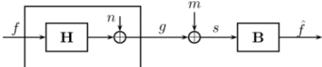
Fig. 1. Measurement and estimation systems model block diagram.
from each other, e.g., we may wish to estimate the field at the outer edges of a region with measurements made in the center.
Measurements are made at the output of the linear system to obtain the measurement vector according to the measurement model
(2) where denotes the measurement noise. We assume that is independent of and . Further, we assume that the compo-nents of are independent, zero-mean random variables, but not necessarily identically distributed. So, the variance of
each component of , indexed by , may be
dif-ferent. Here is an intrinsic part of the relation between and which we have no control over, whereas is the noise asso-ciated with the measurement devices we use and thus depends on the choices we make.
In the following formulation, we assume the knowledge of only second-order statistics of the underlying random variables. We let , and denote the covariance matrices of
, and , respectively. Note that
. Note also that since we assume that has independent
components, .
We assume that the cost associated with measuring the th
component of is , where
de-notes the variance of . The units of are bits. Smaller surement noise levels result in higher costs whereas larger mea-surement noise levels allow lower costs. The plausibility of this form for the cost function is discussed in Section III. The cost of measuring is defined as , the sum of the costs of measuring all of its components.
The objective is to minimize the mean-square error (MSE) between and , the estimate of given . We consider only linear minimum mean-square error (LMMSE) estimators, and denotes the LMMSE estimator. Hence, the estimate may
be written as where is an by matrix. A
block diagram illustrating this problem is given in Fig. 1. The problem can be stated as follows: Given the covariance
matrices , and a system matrix
, determine
(3) (4) subject to
(5)
where is the covariance of
denotes expectation with respect to , and denotes Eu-clidean norm, and tr denotes the trace operator. is the total cost budget; the sum of the cost of all detectors is not allowed to
exceed . We go from (3) to (4) by writing
. A list of selected variables and parameters is given in Table I.
We note that for a given , the minimization over in (4)
is a standard LMMSE problem with solution .
This standard solution may be arrived at using the orthogonality
condition , where
. Hence, we obtain:
(6) subject to (5). In other words, our aim is to minimize the es-timation error by allocating a given measurement cost budget optimally over the components of (2). This is equivalent to optimally adjusting the measurement noise level for each com-ponent, realizing that with a given budget, we cannot measure all components as highly accurately as we wish. Although not ex-plicitly stated, the number of components we actually measure is also an optimization variable. If as the result of our optimiza-tion we find that for certain components, this means that measuring those components do not usefully contribute to the estimation and therefore need not be measured in the first place.
As seen above, this problem differs from a standard LMMSE estimation problem in that the covariance of the measure-ment noise is subject to optimization. We are allowed to “de-sign” the noise levels of the measurement devices subject to a total cost constraint so as to minimize the overall estimation error. To the best of our knowledge this problem is novel.
Our formulation can be easily generalized to allow repeated measurements (more than one measurement of any is al-lowed); however repeated measurements always yield higher error for a given cost budget hence including them in the model does not provide a better performance. This point is discussed in Section IV-1).
III. COSTFUNCTION
What we refer to as a measurement device is an instrument which can measure the value of a scalar physical quantity over some range with some resolution in amplitude. The cost of a measurement device is primarily determined by the number of amplitude levels that the device can reliably distinguish, a no-tion which is sometimes referred to as its dynamic range (al-though the term is sometimes also used to refer to an interval). We will assume that the ranges of measurement devices can be chosen freely to match any interval, and that this has no effect on the cost of the measurements provided the number of resolvable levels remains the same (similar to scaling the range of a multi-meter). For a given linear system, the ranges of the measurement devices depend only on the given covariances. Therefore, they need to be changed only if the covariances change. Given the variances of and in the measurement process , the number of distinguishable levels can be quantified as
(7) where is a constant that depends on how reliably the levels need to be distinguished. In using this expression we are
TABLE I
SELECTEDVARIABLES ANDPARAMETERS
following the same rationale used to define the number of dis-tinguishable signal levels at the receiver of an additive noise channel, which is due to Hartley [29], and further discussed in [30] and [31]. The square-root in the expression keeps the number of levels invariant under scaling of the signals by any constant. Clearly, in the limit of very noisy measurements, should be 1; therefore, we set henceforth.
We now list some properties that any plausible cost function must possess.
1) must be a nonnegative, monotonically increasing function of , with since a device with one measurement level gives no useful information.
2) For any integer , we must have .
This is because a measurement device with levels can be used times in succession with range adjustments between measurements, to distinguish levels. (We also note that this property may be expressed in a more general form as
.)
A function possessing these properties is the logarithm func-tion; therefore we propose
(8) as the cost of carrying out a measurement .
The proposed cost function has the same form as Shannon’s formula for the capacity of a Gaussian noise channel. This does not come as a surprise since a measurement process
is analogous to sending a message across a communication channel that adds a noise term to it. On the other hand, the notion of adjusting the range while keeping the number of re-solvable levels constant has no direct counterpart in the com-munication setting; hence, the measurement and communica-tion problems are not identical problems. We believe such a cost function has never been used to model the cost of measurement devices.
In the communication problem, the amount of information delivered to the receiver is measured by the mutual
re-ceived signals. is also an attractive candidate for the cost function in the measurement scenario since the value of a mea-surement would be quantified most fairly by how many bits of information it actually conveys on the average about the mea-sured quantity. On the other hand, there is a practical difficulty in charging a fee as it depends on the actual probability distribution of the measured quantity. It is logical that the measurement device manufacturer will try to sell its device at the price where the maximum is calculated sub-ject to a power constraint . The would-be equipment purchaser on the other hand will not be willing to pay more than since she or he is only assured that . Shannon [30] shows that this minmax problem is solved by the Gaussian densities for both and and the resulting minmax value is the expression given in (8). Thus, the cost function we propose has a satisfying economic interpretation: the seller of the equipment assumes that the chaser will make the best use of the equipment while the pur-chaser assumes that the equipment will give the worst type of measurement noise (which is Gaussian) for the given level of resolution.
Since Gaussian error is an acceptable model for many types of measurement devices, the cost function that we use makes sense in a wide range of contexts. For problems where measurement noise is known to follow a different distribution, the cost func-tion can be modified accordingly.
Finally we explore the relationship of the measurement problem to rate-distortion theory. It is clear from Fig. 1 that, by the data-processing theorem [32], we have the following relationship regarding the mutual information of the related
random vectors: ; i.e., the estimate can
only provide as much information about as the measurement devices extract from the observable . In turn, by standard
ar-guments, we have . The cost function
that we use upper-bounds
whenever the measurement noise is Gaussian with a given variance and the variance of the measured quantity is fixed as . Thus, for Gaussian measurement noise, we have
where is the total measurement budget. The goal of measurements is the minimization of the MSE
within a budget where denotes . From a rate-distortion theory viewpoint, interpreting as a distortion measure, this is similar to minimizing the av-erage distortion in the reconstruction of from a representation subject to a rate constraint . This viewpoint
im-mediately gives the bound where
is the distortion-rate function applicable to this situation. In the rate-distortion framework one is given complete freedom in forming the reconstruction vectors subject only to a rate constraint, which in measurement terminology would mean the ability to apply arbitrary transformations on the ob-servable before performing a measurement (so as to carry out the measurement in the most favorable coordinate system), and not being constrained to linear measurements or linear estima-tors. Thus, the measurement problem can be seen as a deviation from the rate-distortion problem in which the formation of the reconstruction vector is restricted by various constraints.
IV. SPECIALCASES
1) Repeated Measurements of the Field at a Single Point: As noted, repeated measurements of components of are always suboptimal in the sense that doing so results in greater error for given cost. Here we allow more than one measurement of any component of and show that this is indeed the case. We assume that different measurements are statistically independent condi-tional on even if repeated measurements of the same compo-nent are in question.
First we consider the simple case in which repeated measure-ments are made at a single point and the other components of are not measured. That is, one is allowed to make
measure-ments on indexed by as subject to
the usual cost constraint. Here the subscript denotes the index of the component of where the repeated measurements are made. Since no other component of is measured, the total number of measurements is equal to the number of repeated components
, the measurement noise vector
, and the measurement vector .
We consider the problem of estimation of a single component of the input field where . By studying this case, we wish to see which measurement strategy is better: i) to make one high quality measurement by renting the best device within budget limits, or ii) to split the budget among multiple lower quality devices. Simple LMMSE analysis shows that the first alternative is better, as we now show.
For any given allocation of noise variances , the measurements yield the LMMSE estimate
where . Here, the components of are obtained by solving the orthogonality conditions:
(9)
where . The associated MSE is
(10) The total measurement cost for this scheme is . We observe that among all schemes of allocation of noise variances yielding the same (hence giving the same MSE), the cost is minimized by taking for any one of the indexes and
for the others. This corresponds to making one high quality measurement. Therefore, for a given error, the total cost is minimized by making one high quality measurement rather than many low quality ones. The error is a strictly decreasing function of the cost so that we can further conclude that this is also the strategy minimizing error for given cost.
We note that this result trivially holds when one wants to es-timate the whole field vector instead of a single com-ponent of the vector. It also remains true when other compo-nents of are measured alongside with , as can be shown by noting that the estimation errors for the components of do not change as long as is the same, so that the estimator coeffi-cients associated with these components and therefore the esti-mation error for also do not change. Therefore, we conclude
that allowing repeated measurements of the same point does not provide an opportunity for further optimization, since for every measurement scheme involving more than one measurement of the same component, it is certain that there is another scheme that yields the same error with a lower cost budget.
2) Diagonal Case: In order to see the relationship of our for-mulation with the “water-filling” solutions common in certain information-theoretic problems (e.g., [32, Ch. 9] and [33, Ch. 13]), we consider the special case where the matrix , the matrix is diagonal, , and is the identity ma-trix.
In this special case, we have separate LMMSE problems tied together by a total cost constraint. By standard techniques [32, Ch. 9], [33, Ch. 13], we obtain the optimal detector vari-ances that minimize the estimation error as
(11) where the parameter is selected so that the total cost is . Notice that for those components for which there is a nontrivial
measurement , we have ,
which is reminiscent of the “water-filling” solutions referred to above.
3) Accurate Measurements (High Budget) Case: When the uncertainty introduced by the measurements are small with re-spect to the range of , we refer to this case as the accurate mea-surements case. This is the case where is near , where is the covariance of . Hence, we may use the first order approximation of the inverse of a positive
def-inite symmetric matrix to write ,
and using the linearity of the trace operator, the MMSE can be written as
(12) The error is expressed as the sum of two parts. The first part is independent of the accuracy of the measurements. For physical phenomena represented by noninvertible matrices , this irre-ducible error remains even if the measurements are perfect, and corresponds to the limited information transfer capability of the physical system. The second additive error component is due to the imperfect measurements. In this case the estimation error is a linear function of , and the resulting optimization problem is convex. Since the objective and constraint functions are differ-entiable and Slater’s condition holds, the Karush–Kuhn–Tucker (KKT) conditions are necessary and sufficient for optimality [34, Ch. 5]. Hence, by solving the KKT conditions, the optimal noise levels can be obtained as
(13) where is a parameter chosen so that the total cost is ,
and ’s are the diagonal elements of .
V. NUMERICALRESULTS
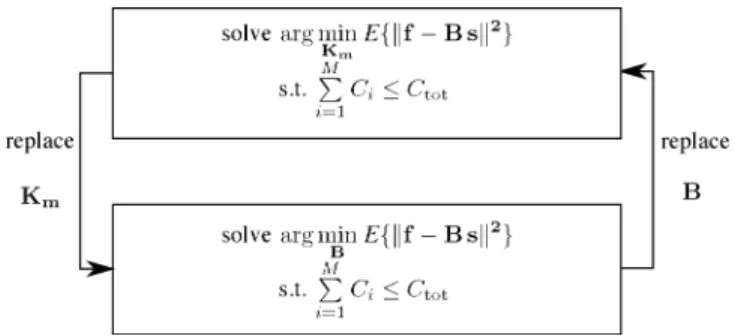
First, we present the algorithm we employed for solving the optimization problem (6). Our algorithm is based on (4) and relies on taking turns in fixing and and minimizing over
Fig. 2. Block diagram of the algorithm.
the other. For fixed , the optimal value of the linear estimator that minimizes the error can be analytically written in terms
of as . On the other
hand, if we fix , the problem is to minimize
over subject to (5). Since the differentiability and Slater’s condition hold in this case as well, the optimal noise levels can be found as
(14) by solving the KKT conditions. Here is a parameter chosen so that the total cost is , and ’s are the diagonal
elements of .
The resulting algorithm is summarized as follows (Fig. 2): We initialize the algorithm by setting and to a random positive-definite diagonal matrix. At each iteration
, first we fix and set where
, which is the optimum value
of for . Then we fix and minimize over : We
obtain by solving (14) with replaced with . For the stopping criterion, we use the relative
error: if does not change by more than
over 10 consecutive iterations, we stop; otherwise, we incre-ment and continue. The algorithm converges typically within 10–150 iterations depending on the problem parameters. Details on this type of algorithm may be found in [35, Ch. 9].
The problem we formulate and solve in this paper was moti-vated by the physical problem of measuring propagating wave fields at a certain number of points and estimating the values of the field, possibly at other, distant locations. Although our formulation can handle very general cases of this problem, in our numerical examples we will focus on the case where there are two planar or spherical reference surfaces, perpendicular to the axis of propagation and separated by a certain distance. We assume that all measurement probes are placed uniformly on one surface and we desire to estimate the field on the other sur-face. In this case the measured field is related to the unknown field through a diffraction integral, a convenient approximation of which is the Fresnel diffraction integral or more generally a quadratic-phase integral (linear canonical transform) [36, Ch. 8], [37, Ch. 2], and [38], [39]. It is well known that these inte-grals can be expressed in terms of the fractional Fourier trans-form (FRT), which provides an elegant and pure description of these systems [40, Ch. 9], [41], and which has found many ap-plications in signal processing [42]–[49]. The FRT is the frac-tional operator power of the Fourier transform with fracfrac-tional
order . When the FRT reduces to the identity operation and when it reduces to the ordinary Fourier transform. Moreover, the transform is index-additive: the th transform of the th transform is equal to the th transform. Fur-ther information on the FRT and its computation may be found in [40] and [50]. Essentially, the FRT captures the underlying physics of wave propagation and diffraction phenomena in its purest form and is therefore suitable for modeling wave propa-gation for our present purposes. Thus, in our examples we will take the system matrix to be the by real equivalent of the by complex FRT matrix. For the generation of FRT matrices of different orders, an implementation of the algorithm presented in [51] and in [40, Ch. 6] is used; this implementation is available at [52].
Propagating wave-fields may have different degrees of what is known as coherence. Highly coherent fields are those whose values at different points are highly correlated with each other. Highly incoherent fields are those whose values at different points are highly uncorrelated. Since we have observed that our results depend on the degree of coherence of the fields, we will consider several covariance matrices corresponding to different degrees of coherence (correlation between their components). It is known that highly coherent fields have covariance matrices whose eigenvalues are highly unevenly distributed. On the other hand, highly incoherent fields have eigenvalues which are nearly equal to each other [53]. To obtain covariance matrices with different degrees of coherence, we will choose the eigen-values to be normally distributed with standard deviation equal to pixels. Here the parameter can also be interpreted as the number of standard deviations of the Gaussian covered by the samples. In our experiments takes the values , where corresponds to the case where all but one eigenvalue is negligible, and
corresponds to the case where all eigenvalues are nearly equal. While is a convenient parameter to work with, we note that it should not be seen as a linear measure of the degree of coherence [53]. To generate the covariance matrices with these eigenvalues, we use the eigenvalue-eigenvector decomposition
of a covariance matrix , where .
Here the orthogonal matrix is obtained by QR decomposition of a matrix with i.i.d. zero-mean Gaussian entries. For the system noise , the covariance matrix is generated similarly with with a different matrix.
Another important parameter used in the experiments is (15)
where the second form follows from which in turn follows from the unitarity of the FRT. SNR measures the ratio of signal power to inherent system noise power, before measure-ments.
In the following experiments our main purpose will be to in-vestigate the tradeoff between the MSE error and mea-surement cost budget after we have optimized over all pos-sible allocations of cost over the measurement devices. The error will be reported as a percentage defined as . The cost budget is measured in bits by taking logarithms to base 2. Unless otherwise stated all experiments are made with
and .
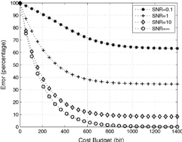
Fig. 3. Experiment 1: Error versus cost forN = M = 256; a = 0:5; = 0:25, SNR variable.
Fig. 4. Experiment 1: Error versus cost forN = M = 256; a = 0:5; = 1024, SNR variable.
Exp. 1: This experiment investigates the effect of SNR on the tradeoff between and . In this experiment, SNR was variable, ranging over 0.1, 1, 10, and two different values of were considered. Figs. 3 and 4 give the curves for low and high values, respectively. We notice that for both of the cases is very sensitive to increases in for smaller . Then it becomes less responsive and eventually saturates to the error value corresponding to zero measurement noise. For each value of cost, the error decreases as SNR increases, and for higher cost values will approach zero as . We see that when the field is more highly coherent (Fig. 4), we obtain much better tradeoff curves for all values of SNR than Fig. 3 which represents the highly incoherent extreme. For instance for , for the highly incoherent field an error of 10% is obtained at a cost of 400 bits, whereas for the highly coherent field the same error is achieved at a cost lower than 5 bits. This point is further investigated in Exp. 2.
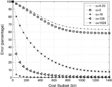
Fig. 5. Experiment 2: Error versus cost forN = M = 256; a = 0:5; SNR = 0:1; variable.
Fig. 6. Experiment 2: Error versus cost forN = M = 256; a = 0:5; SNR = 1; variable.
Exp. 2: This experiment investigates the effect of degree of coherence of the unknown field on the tradeoff between and . Figs. 5 and 6 show the results for two
different SNR values ( and ), for
. Both of the plots show that for low values of corresponding to lower degrees of coherence, it is more difficult to achieve low values of error within a given budget. But as increases, the total uncertainty in the field decreases, and it becomes a lot easier to achieve lower values of error. In fact, for high values of and for low values of budget, the optimal strategy to minimize error turns out to be to measure the field value at only a few points with more accurate (and costly) measurement devices, rather than spreading the cost budget among many measurement points. This observation is further investigated in Exp. 4.
It is interesting to note that in all of the numerical examples we have considered, including the incoherent case, it is possible to reach with an average of 4 bits per component, the same error level that would be achieved with infinite accuracy (and cost).
Comparing the performances in Figs. 5 and 6 for low and high values of the cost budget, we see that for low budget values the effect of degree of coherence of the field can be considered more pronounced in the high SNR case, whereas for high budget values this effect is more pronounced in the low SNR case: For high values of cost budget, it is always possible to obtain very low values of error regardless of degree of coherence, when the SNR is high. But when the SNR is low and the cost budget is high, a substantial performance difference is observed between the correlated and uncorrelated fields, since it is pos-sible to effectively cancel the effect of system noise when the degree of coherence of the field is high, yielding a better perfor-mance. When the budget is small and the SNR is low, although highly correlated fields lead to better performance, this improve-ment is limited by the presence of noise. When the budget is small but SNR is high, it is possible to obtain very low values of error when the field is highly correlated, resulting in a far better performance compared to the uncorrelated case.
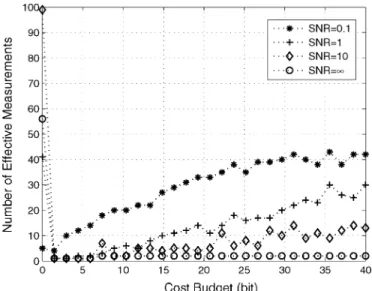
Exp. 3: This experiment investigates the effect of SNR on the relationship between the number of effective measurements and the budget . We will consider a measurement at a point to be effectively made if the cost of the measurement at this point is greater than bits. With this choice of threshold, it is guaranteed that the total cost of the measure-ments that are effectively made is higher than . We use . Measurements with less cost are very noisy mea-surements and do not contribute much either to the quality of the estimate or the total cost, so that it does not make much differ-ence whether we actually perform them or not.
For , we see that one has to do measurements at all of the measurement points for all values of SNR and for all values of . This result is plausible since the field values are nearly uncorrelated in this case, and each point can be considered to provide new information.
The case of highly coherent fields is more interesting. Fig. 7
shows the results for with . For
low values of SNR, the optimal strategy is to split the budget relatively broadly among the points. On the other hand, for high values of SNR, the best strategy is to allocate the budget to a smaller number of points. To understand this behavior, we observe that in this experiment the field values are highly cor-related, hence the points measured carry nearly the same infor-mation. On the hand the system noise is highly uncorrelated. Based on these two observations, we can say that measuring a larger number of points increases the averaging effect and thus suppression of the system noise. Successively measuring highly correlated variables normally adds little information [so that one would prefer fewer but more accurate measurements instead]. However, when there is a lot of noise, the benefits of noise sup-pression can outweigh this so that a larger number of measure-ments are preferred.
Although the curves behave as if the number of effective measurements saturate at an asymptote for high values of cost budget, this is in fact not true and the number of effective mea-surements continue to increase as budget increases. This point is further discussed in the next experiment.
Exp. 4: This experiment investigates the effect of de-gree of coherence of the unknown field on the rela-tionship between the number of effective measurements and the budget . Fig. 8 shows the results for
Fig. 7. Experiment 3: Effective number of measurements versus cost forN = M = 256; a = 0:5; = 1024, SNR variable.
Fig. 8. Experiment 4: Effective number of measurements versus cost forN = M = 256; a = 0:5; SNR = 0:1; variable.
. We see that for all values of , and for low values of cost budget, the best strategy is to measure more accurately a relatively smaller number of points. But as the budget increases, the information that can be gained by measuring the field at a limited number of points with greater and greater accuracy saturates and splitting the budget over a larger number of measurement points become beneficial. For low values of , this shift in strategy takes place at lower values of cost budget. For a highly coherent field, the measurement of the field value at a particular point says much more about the field values at other points, and the benefit of measuring some of the field values with greater accuracy is prevailing.
Comparing this plot with Fig. 5 shows that the increase in the number of effective measurements for higher values of budget is not very meaningful since, for these budget values the error has almost reached its saturation value, but the algorithm being blind to this fact, increases the number of effective measure-ments to achieve tiny decreases in error. For instance, with
Fig. 9. Experiment 5: Error versus cost forN = M = 256; a = 0:5; = 1024, SNR variable. The dotted lines are for optimal cost allocation and the corresponding solid lines are for uniform cost allocation.
, the error reaches a value of almost zero for a cost budget of 200 bits, and beyond this cost budget any increase in the number of measurements is made for the sake of a very small perfor-mance improvement.
We have also repeated the above experiment made for for other values of SNR. We have observed that as SNR increases, a similar behavior is observed: the number of effec-tive measurements again increases with increasing budget for all values of . But this time the rate of increase of the number of ef-fective measurements with increasing budget is smaller. Also, at a given cost budget, the ratio of the number of effective measure-ments is larger for different values of . Hence, the difference in the optimum cost allocation strategies for different values of
is more apparent for higher values of SNR.
Exp. 5: This experiment aims to demonstrate how applying the optimum cost allocation strategy we have employed up to this point, improves the tradeoff between and com-pared to a simple uniform cost allocation strategy, where the cost
budget is equally allocated: . We
expect that use of the optimal cost allocation will make a bigger difference for more highly coherent fields, since Exp. 4 shows that the optimum cost allocation is drastically different from a uniform cost allocation scheme. Furthermore, Exp. 3 suggests this effect should be more pronounced when SNR is high. Fig. 9 compares the tradeoff curves with optimum and uniform cost
allocation schemes with . The
dashed curves and the straight lines show the results for the op-timum cost allocation scheme and the uniform cost allocation scheme respectively. As expected, for all values of SNR, the optimum cost allocation scheme gives significantly better trade-offs compared to the uniform cost allocation case. For low values, as SNR increases, the ratio of percentage error corre-sponding to uniform cost allocation to that correcorre-sponding to op-timum cost allocation increases, showing that when the degree of coherence is high and the system noise is small, it is more important to optimize the allocation of the budget to the mea-surement points.
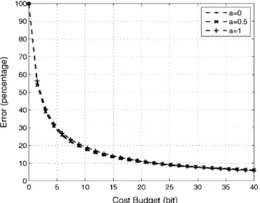
Exp. 6: This experiment investigates the effect of the frac-tional Fourier order on the tradeoff between and .
Fig. 10 presents the tradeoff curves with ,
Fig. 10. Experiment 6: Error versus cost forN = M = 256; SNR = 0:1; = 1024; a variable.
values of are very close to each other, although higher values of yield slightly better curves. We have also repeated this experiment for different values of and SNR. The resulting tradeoff curves in these other experiments exhibit even less dif-ference for different FRT orders. Remembering that is a mono-tonic increasing function of the distance of propagation in wave propagation problems, these results show that the MSE is not critically dependent on how far the measurement devices are placed along the propagation axis.
Exp. 7: This experiment investigates the effect of making measurements at a smaller number of points. More specifically,
we will examine the dependence of on for a
fixed . Fig. 11 shows the results for
and .
The measurement locations were chosen as uniformly spaced subgrids of the full 256-point grid (i.e., the grid for
was a sub-grid of that for which was a sub-grid of
that for , etc.). We see that for and
roughly the same performance with the
case is observed, whereas for other values the performance de-grades with decreasing . This behavior is related to the ef-fective number of nonzero eigenvalues. For , the eigen-values are samples of a Gaussian with standard deviation 256/16 pixels. Assuming the values of a Gaussian beyond its third stan-dard deviation are negligible, the covariance matrix has about nonzero eigenvalues. Indeed we observe that as long as the number of measurements is higher than 48, the tradeoff curves are similar to the case. But if we restrict ourselves to do measurements at a smaller number of points such as , a substantial performance degra-dation is observed.
VI. CONCLUSION
Motivated by problems related to measurement of propa-gating wave-fields, we formulated the problem of optimally measuring observed variables so as to estimate unknown vari-ables under a total cost constraint. We proposed a measurement device model where each device has a cost depending on its resolving power. Based on this cost function we determine the
Fig. 11. Experiment 7: Error versus cost forN = 256; a = 0:5; = 16; SNR = 1; M variable.
number of measurement devices and their accuracies that mini-mize estimation error for given total cost. We produce tradeoff curves between the error and the cost budget, corresponding to the optimal measurement strategy. We discuss the effects of SNR, distance of propagation, and the degree of coherence of the wave-fields on these tradeoffs.
Specific hardware may deviate from our hardware-indepen-dent cost-budget model to varying degrees. However, all mea-surement devices have finite accuracy and in general their cost is an increasing function of their accuracy. Therefore, we believe that the nature of the tradeoffs observed and the general con-clusions and insights will remain useful under a wide variety of circumstances.
We have seen that making measurements with higher quality (and cost) measurement devices, should be preferred over making repeated measurements with lower cost (and quality) devices. This helps explain why it is better to make a limited number of high quality measurements when the field is highly coherent. At the other extreme of coherence, when the fields are uncorrelated, we noted that the best measurement strategy is a reverse-water filling scheme.
As expected, in our numerical experiments we observe that the estimation error decreases with increasing cost budget, and reaches zero error when there is no system noise. Not surpris-ingly, with increasing system noise levels (decreasing SNRs), poorer tradeoffs are observed. The cost-error tradeoff is greatly degraded by decreasing SNR for relatively incoherent fields, whereas it can be said to be less sensitive to SNR for coherent fields.
In general, it is possible to obtain better tradeoff curves for relatively coherent fields as compared to relatively incoherent fields for all values of SNR. The difference can be quite sub-stantial and in the limit of full coherence/incoherence very large. For instance, for a coherent field, a total cost of a few bits may be sufficient to obtain a certain error, whereas for an incoherent field one may need a total cost which is of the order of times as large as this to achieve the same error. For relatively incoherent fields the best measurement strategy is to measure a greater number or most of the field components, whereas for relatively
coherent light it is better to allocate the cost budget among a smaller number of field components. How small a number also depends on the SNR. It is preferable to measure a somewhat larger number of components when the SNR is low, but still many of the field components remain effectively unmeasured. These observations underline the fact that the degree of coher-ence (correlation) is a fundamental parameter that can have a significant effect on the results and therefore should be taken into consideration in order to ensure general applicability.
We also observed that in the wave propagation context the tradeoff curves are not significantly affected by how far from the unknown field the measurements are made. This allows us flexibility to accommodate practical constraints when choosing the measurement locations.
Finally we briefly discuss the relationship of the problem ad-dressed in this paper with some earlier works which also in-volve estimation of desired quantities from measurements made from multiple sensors transmitting their observations to a deci-sion center. The design of sensor and fudeci-sion center strategies has been studied in the context of different setups with different communication, computation, and power constraints [54]–[66]. A number of these works share some of the features of our for-mulation. In [56] and [59], problems related to wave propaga-tion are studied with a statistical signal processing approach. Optimal sensor design has been studied in the form of quantizers or local encoders; for instance [54] and [55]. The problem of sensor selection as an estimation problem is considered in [63], and under given sensor performance and costs as a detection problem in [64]. The tradeoff between performance and total bit rate with a special emphasis on quantizer bit rates is studied in [57] and [58], where the estimation of a single parameter is considered. Although various aspects of the problem of sensing of physical fields have been widely studied as estimation prob-lems, much of this work has loose connections with both the underlying physical phenomena and the physical aspects of the sensors employed. There seems to be a disciplinary boundary between these works and the works cited in Section I. Further work to bridge these two approaches will help us better under-stand the information theoretic relationships in physical fields and their measurement from a broader perspective.
REFERENCES
[1] G. T. Di Francia, “Resolving power and information,” J. Opt. Soc.
Amer., vol. 45, pp. 497–501, Jul. 1955.
[2] D. Gabor, “Light and information,” in Progress in Optics, E. Wolf, Ed. Amsterdam, The Netherlands: Elsevier, 1961, vol. I, pp. 109–153, ch. 4.
[3] F. Gori and G. Guattari, “Shannon number and degrees of freedom of an image,” Opt. Commun., vol. 7, pp. 163–165, Feb. 1973.
[4] A. Starikov, “Effective number of degrees of freedom of partially co-herent sources,” J. Opt. Soc. Amer., vol. 72, pp. 1538–1544, 1982. [5] O. Bucci and G. Franceschetti, “On the degrees of freedom of scattered
fields,” IEEE Trans. Antennas Propag., vol. 37, pp. 918–926, Jul. 1989. [6] D. Mendlovic and A. W. Lohmann, “Space-bandwidth product adapta-tion and its applicaadapta-tion to superresoluadapta-tion: Fundamentals,” J. Opt. Soc.
Amer. A, vol. 14, pp. 558–562, Mar. 1997.
[7] R. Piestun and D. A. B. Miller, “Electromagnetic degrees of freedom of an optical system,” J. Opt. Soc. Amer. A, vol. 17, pp. 892–902, May 2000.
[8] A. Poon, R. Brodersen, and D. Tse, “Degrees of freedom in multiple-antenna channels: A signal space approach,” IEEE Trans. Inf. Theory, vol. 51, pp. 523–536, Feb. 2005.
[9] J. Xu and R. Janaswamy, “Electromagnetic degrees of freedom in 2-D scattering environments,” IEEE Trans. Antennas Propag., vol. 54, pp. 3882–3894, Dec. 2006.
[10] M. Migliore, “On the role of the number of degrees of freedom of the field in MIMO channels,” IEEE Trans. Antennas Propag., vol. 54, pp. 620–628, Feb. 2006.
[11] R. Kennedy, P. Sadeghi, T. Abhayapala, and H. Jones, “Intrinsic limits of dimensionality and richness in random multipath fields,” IEEE
Trans. Signal Process., vol. 55, no. 6, pp. 2542–2556, Jun. 2007.
[12] A. Stern and B. Javidi, “Analysis of practical sampling and reconstruc-tion from Fresnel fields,” Opt. Eng., vol. 43, pp. 239–250, Jan. 2004. [13] L. Onural, “Exact analysis of the effects of sampling of the scalar
diffraction field,” J. Opt. Soc. Amer. A, vol. 24, pp. 359–367, Jan. 2007. [14] D. MacKay, “Quantal aspects of scientific information,” IEEE Trans.
Inf. Theory, vol. 1, pp. 60–80, Feb. 1953.
[15] J. T. Winthrop, “Propagation of structural information in optical wave fields,” J. Opt. Soc. Amer., vol. 61, pp. 15–30, Jan. 1971.
[16] T. W. Barret, “Structural information theory,” J. Acoust. Soc. Amer., vol. 54, pp. 1092–1098, Oct. 1973.
[17] M. S. Hughes, “Analysis of digitized wave-forms using Shannon en-tropy,” J. Acoust. Soc. Amer., vol. 93, pp. 892–906, Jan. 1993. [18] D. Blacknell and C. J. Oliver, “Information-content of coherent
im-ages,” J. Phys. D, vol. 26, pp. 1364–1370, Jan. 1993.
[19] F. T. Yu, Entropy and Information Optics. New York: Marcel Dekker, 2000.
[20] R. Konsbruck, E. Telatar, and M. Vetterli, “On the multiterminal rate-distortion function for acoustic sensing,” in Proc. IEEE Int. Conf.
Acoust., Speech Signal Process. (ICASSP), 2006, vol. 4, pp. 701–704.
[21] L. Hanlen and M. Fu, “Wireless communication systems with-spatial diversity: A volumetric model,” IEEE Trans. Wireless Commun., vol. 5, pp. 133–142, Jan. 2006.
[22] M. Jensen and J. Wallace, “Capacity of the continuous-space elec-tromagnetic channel,” IEEE Trans. Antennas Propag., vol. 56, pp. 524–531, Feb. 2008.
[23] F. Gruber and E. Marengo, “New aspects of electromagnetic informa-tion theory for wireless and antenna systems,” IEEE Trans. Antennas
Propag., vol. 56, pp. 3470–3484, Nov. 2008.
[24] M. Migliore, “On electromagnetics and information theory,” IEEE
Trans. Antennas Propag., vol. 56, pp. 3188–3200, Oct. 2008.
[25] E. D. Micheli and G. A. Viano, “Inverse optical imaging viewed as a backward channel communication problem,” J. Opt. Soc. Amer. A, vol. 26, pp. 1393–1402, Jan. 2009.
[26] A. Özçelikkale, “Structural and metrical information in linear sys-tems,” Master’s thesis, Bilkent Univ., Ankara, Turkey, 2006. [27] A. Özçelikkale, H. M. Özaktas¸, and E. Arıkan, “Measurement
strate-gies for input estimation in linear systems,” in Proc. 2007 IEEE Signal
Process. and Commun. App. Conf. (in Turkish) Transl.: Do˘grusal
sis-temlerde girdi kestirimi ˙Için ölçüm yöntemleri, pp. 1–4.
[28] A. Özçelikkale, H. M. Ozaktas, and E. Arıkan, “Optimal measurement under cost constraints for estimation of propagating wave fields,” in
Proc. 2007 IEEE Int. Symp. Inf. Theory, pp. 696–700.
[29] R. V. L. Hartley, “Transmission of information,” Bell Syst. Tech. J., vol. 7, pp. 535–563, Jul. 1928.
[30] C. E. Shannon, “A mathematical theory of communication,” Bell Syst.
Tech. J., vol. 27, pp. 379, 623–423, 656, Jul.–Oct. 1948.
[31] B. M. Oliver, J. R. Pierce, and C. E. Shannon, “The philosophy of PCM,” in Proc. I.R.E., Nov. 1948, vol. 36, pp. 1324–1331.
[32] R. G. Gallager, Information Theory and Reliable Communication. New York: Wiley, 1968.
[33] T. M. Cover and J. A. Thomas, Elements of Information Theory. New York: Wiley, 1991.
[34] S. Boyd and L. Vandenberghe, Convex Optimization. New York: Cambridge Univ. Press, 2004.
[35] J. Nocedal and S. J. Wright, Numerical Optimization. New York: Springer, 2006.
[36] P. M. Morse and K. U. Ingard, Theoretical Acoustics. Princeton, NJ: Princeton Univ. Press, 1986.
[37] C. A. Balanis, Antenna Theory: Analysis and Design. New York: Wiley, 2005.
[38] L. Onural and H. M. Ozaktas, “Signal processing issues in diffraction and holographic 3DTV,” Signal Process.: Image Commun., vol. 22, pp. 169–177, Feb. 2007.
[39] M. J. Bastiaans, “Applications of the Wigner distribution function in optics,” in The Wigner Distribution: Theory and Applications in Signal
Processing, W. Mecklenbrauker and F. Hlawatsch, Eds. Amsterdam, The Netherlands: Elsevier, 1997, pp. 375–426.
[40] H. M. Ozaktas, Z. Zalevsky, and M. A. Kutay, The Fractional Fourier
Transform With Applications in Optics and Signal Processing. New York: Wiley, 2001.
[41] H. M. Ozaktas, B. Barshan, D. Mendlovic, and L. Onural, “Convolu-tion, filtering, and multiplexing in fractional Fourier domains and their relation to chirp and wavelet transform,” J. Opt. Soc. Amer. A, vol. 11, pp. 547–559, Feb. 1994.
[42] M. A. Kutay, H. Özaktas¸, H. M. Ozaktas, and O. Arıkan, “The frac-tional Fourier domain decomposition,” Signal Process., vol. 77, pp. 105–109, Aug. 1999.
[43] M. F. Erden, M. A. Kutay, and H. M. Ozaktas, “Repeated filtering in consecutive fractional Fourier domains and its application to signal restoration,” IEEE Trans. Signal Process., vol. 47, pp. 1458–1462, May 1999.
[44] H. M. Ozaktas and U. Sümbül, “Interpolating between periodicity and discreteness through the fractional Fourier transform,” IEEE Trans.
Signal Process., vol. 54, pp. 4233–4243, Nov. 2006.
[45] S. Qazi, A. Georgakis, L. K. Stergioulas, and M. Shikh-Bahaei, “Inter-ference suppression in the Wigner distribution using fractional Fourier transformation and signal synthesis,” IEEE Trans. Signal Process., vol. 55, no. 6, pp. 3150–3154, Jun. 2007.
[46] S.-C. Pei and J.-J. Ding, “Relations between Gabor transforms and frac-tional Fourier transforms and their applications for signal processing,”
IEEE Trans. Signal Process., vol. 55, no. 10, pp. 4839–4850, Oct. 2007.
[47] A. S. Amein and J. J. Soraghan, “Fractional chirp scaling algorithm: Mathematical model,” IEEE Trans. Signal Process., vol. 55, no. 8, pp. 4162–4172, Aug. 2007.
[48] K. K. Sharma and S. D. Joshi, “Uncertainty principle for real signals in the linear canonical transform domains,” IEEE Trans. Signal Process., vol. 56, no. 7, pp. 2677–2683, Jul. 2008.
[49] R. Tao, X.-M. Li, Y.-L. Li, and Y. Wang, “Time-delay estimation of chirp signals in the fractional Fourier domain,” IEEE Trans. Signal
Process., vol. 57, no. 7, pp. 2852–2855, Jul. 2009.
[50] A. Koç, H. M. Ozaktas, C. Candan, and M. A. Kutay, “Digital com-putation of linear canonical transforms,” IEEE Trans. Signal Process., vol. 56, no. 6, pp. 2383–2394, Jun. 2008.
[51] Ç. Candan, M. A. Kutay, and H. M. Ozaktas, “The discrete fractional Fourier transform,” IEEE Trans. Signal Process., vol. 48, no. 5, pp. 1329–1337, May 2000.
[52] Ç. Candan, “Discrete fractional Fourier transform matrix generator,” [Online]. Available: http://www.ee.bilkent.edu.tr/~haldun/dFRT.m Jul. 1998
[53] H. M. Ozaktas, S. Yüksel, and M. A. Kutay, “Linear algebraic theory of partial coherence: Discrete fields and measures of partial coherence,”
J. Opt. Soc. Amer. A, vol. 19, pp. 1563–1571, Aug. 2002.
[54] J.-J. Xiao and Z.-Q. Luo, “Decentralized estimation in an inhomo-geneous sensing environment,” IEEE Trans. Inf. Theory, vol. 51, pp. 3564–3575, Oct. 2005.
[55] A. Ribeiro and G. Giannakis, “Bandwidth-constrained distributed es-timation for wireless sensor networks—Part I: Gaussian case,” IEEE
Trans. Signal Process., vol. 54, no. 3, pp. 1131–1143, Mar. 2006.
[56] S. Nordebo and M. Gustafsson, “Statistical signal analysis for the inverse source problem of electromagnetics,” IEEE Trans. Signal
Process., vol. 54, no. 6, pp. 2357–2361, Jun. 2006.
[57] S. Marano, V. Matta, and P. Willett, “Quantizer precision for dis-tributed estimation in a large sensor network,” IEEE Trans. Signal
Process., vol. 54, no. 10, pp. 4073–4078, Oct. 2006.
[58] J. Li and G. AlRegib, “Rate-constrained distributed estimation in wire-less sensor networks,” IEEE Trans. Signal Process., vol. 55, no. 5, pp. 1634–1643, May 2007.
[59] T. Oliphant, “On parameter estimates of the lossy wave equation,”
IEEE Trans. Signal Process., vol. 56, no. 1, pp. 49––60, Jan. 2008.
[60] T. Aysal and K. Barner, “Constrained decentralized estimation over noisy channels for sensor networks,” IEEE Trans. Signal Process., vol. 56, no. 4, pp. 1398–1410, Apr. 2008.
[61] Y. Wang, P. Ishwar, and V. Saligrama, “One-bit distributed sensing and coding for field estimation in sensor networks,” IEEE Trans. Signal
Process., vol. 56, no. 9, pp. 4433–4445, Sep. 2008.
[62] Z. Quan, W. Kaiser, and A. Sayed, “Innovations diffusion: A spatial sampling scheme for distributed estimation and detection,” IEEE
Trans. Signal Process., vol. 57, no. 2, pp. 738–751, Feb. 2009.
[63] S. Joshi and S. Boyd, “Sensor selection via convex optimization,” IEEE
Trans. Signal Process., vol. 57, no. 2, pp. 451–462, Feb. 2009.
[64] M. Lazaro, M. Sanchez-Fernandez, and A. Artes-Rodriguez, “Optimal sensor selection in binary heterogeneous sensor networks,” IEEE
Trans. Signal Process., vol. 57, no. 4, pp. 1577–1587, Apr. 2009.
[65] V. Cevher and L. M. Kaplan, “Acoustic sensor network design for po-sition estimation,” ACM Trans. Sensor Netw., vol. 5, pp. 1–28, May 2009.
[66] H. Zhang, J. Moura, and B. Krogh, “Dynamic field estimation using wireless sensor networks: Tradeoffs between estimation error and communication cost,” IEEE Trans. Signal Process., vol. 57, no. 6, pp. 2383–2395, Jun. 2009.
Ayça Özçelikkale (S’01–M’10) received the B.S.
de-gree from Middle East Technical University, Ankara, Turkey, in 2004 and the M.S. degree from Bilkent University, Ankara, Turkey in 2006, both in electrical engineering.
She is currently working towards the Ph.D. degree in Bilkent University, Ankara, Turkey. Her research interests are in the area of signal processing.
Haldun M. Ozaktas (M’07) received the B.S.
de-gree from Middle East Technical University, Ankara, Turkey, in 1987 and the Ph.D. degree from Stanford University, Stanford, CA, in 1991.
He joined Bilkent University, Ankara, Turkey, in 1991, where he is presently a Professor of electrical engineering. In 1992, he was at the University of Erlangen-Nurnberg, Bavaria as an Alexander von Humboldt Foundation Postdoctoral Fellow. During summer 1994, he worked as a Consultant at Bell Laboratories, Holmdel, NJ. He is the author of over 90 refereed journal articles, over ten book chapters, and over 100 conference presentations and papers, over 35 of which have been invited. He is also author of the book The Fractional Fourier Transform (Wiley, 2001) and edited the book Three-Dimensional Television (Springer, 2008). His academic interests include signal and image processing, optical information processing, and optoelectronic and optically interconnected computing systems.
Dr. Ozaktas has a total of over 3000 citations to his work recorded in the Science Citation Index (ISI). He is the recipient of the 1998 ICO International Prize in Optics and one of the youngest recipients ever of the Scientific and Tech-nical Research Council of Turkey (TUBITAK) Science Award (1999), among other awards and prizes. He is also one of the youngest members of the Turkish Academy of Sciences and a Fellow of the Optical Society of America (OSA). He has served as an Associate Editor of the IEEE TRANSACTIONS ONSIGNAL
PROCESSING.
Erdal Arıkan (S’84–M’86–SM’94) was born in
Ankara, Turkey, in 1958. He received the B.S. degree from the California Institute of Tech-nology, Pasadena, CA, in 1981, and the S.M. and Ph.D. degrees from the Massachusetts Institute of Technology, Cambridge, MA, in 1982 and 1985, respectively, all in electrical engineering.
Since 1987, he has been with the Electrical–Elec-tronics Engineering Department of Bilkent Univer-sity, Ankara, Turkey, where is currently a Professor. His research interests are in information theory and communication systems.