Single machine total tardiness problem: exact and heuristic algorithms based on Beta-sequence and decomposition theorems

Й ^ "* >· .ν·»·'ΐΐι,·,ΐ·.ί«*.; « « V /w »»м^· ^ ^ í ·. j . » S· У й' mí' Ыі> il 'W .Ѵ·!' ■ ".•.іч ' ; ■ : ' ’· ■; - ; ·; w ' 'П·' '~Т^' tíííí5 ¿ л W N«· .4 Ч.А' Ь ■ «■ ί Λ lí.*^ ;,'i> . ) /: Τ · *';** ’ w*'» ¿ ΰ ¿ : i ·!*,я ’<'■.(· . · " L' -'‘ . i ; f i · -¿ ч'Лі i i v V». ; ;. » ■ Λ··5' Ч Îi Г' ■-•J ·ί ί ■': :■ > !;·"| ! .· > ν * O e ^ ^jí '» ■ 4uC if Ч«*' w W ' iil i t 'i i <4 »'<< я м ;ύβ С . J - ; ^Рі'^щккА- vvr i f ù 4 ‘4', ;; й’ і і 'уЧ · <І».^' «4 s fc i r i» о '.’· -W*^ tí 4 o ' ■ ,■'< л . ·"' ^ І'’а » ıJÎ ‘.Sİ A vf’ J *‘/ · ^¿1 ':;if '· \ · - ] / ' ."i ■. : j ·· ·■' : "l . . к " . ' ■· ’'' ' 0 0 « <¿)i 4 y .; Ч si ' Л.І- iT « 4 4f \ J t -4 . y ■ іф,·' «İM *1*«, Ψ ^·ώ 'У-я «¿K< ■< у У •Ü ί· Ч і ; '! ‘ N•■1 О' Ѵ -i .1·' «А Л (I '-·.>' '« 'i У i l t t '·» y «'■■·* ¿-a· / ki S**'■] •«J» U И «ад / J " j í Ш ^ г-1'чГуЧі 'u í· . Ä .·,* ’ .li íc '•♦ií' y »»,■%*..;· ■; ¡,» !,чі : .v _!·■ ' > -дѴ, '· ϊ ·. f · й. ■·.'. к ^ я я . ; V · ν ■ѴѵѴ',.« ;·*)■, . ', ·■;' ! i ■ · · .4 . . . .< ''· ίβ ИІ it İM* ¡k Ш w .«і*' ч< »'Ί1 чМ А% «4 <Ы» я Ч й 'ям* ■ ^ Í r j í ’ í? f ';■’■ > í· 1·^ ; ; / ,'.а >( ' «f Ht W »i W ¿ Il «. w « ьм*· 1İ.í^ \ І ч * '> i w *«? ЛІ j ··· .'·' :‘1 if i •^•'>: ·? « ,*·^^ ; ^ ··. >'* -fu ■·■ ·.·?* .’ V ·! :·?* il . '; }-:іл ¿J ¿»«.Οι» >. ·.: ..;* V. ‘ !^ ■ ;■ *»■ ·:. / ··.» .. f.'.. · ·.'

SINGLE MACHINE TOTAL TARDINESS PROBLEM:

EXACT AND HEURISTIC ALGORITHMS BASED ON

/^-SEQUENCE AND DECOMPOSITION THEOREMS

A THESIS

SUBMITTED TO THE DEPARTMENT OF INDUSTRIAL ENGINEERING

AND THE INSTITUTE OF ENGINEERING AND SCIENCES OF BILKENT UNIVERSITY

IN PARTIAL FULFILLMENT OF THE REQUIREMENTS FOR THE DEGREE OF

MASTER OF SCIENCE

By

Bahar Kara

September, 1994

n

I certify that I have read this thesis and that in my opinion it is fully adequate, in scope and in quality, as a thesis for the degree of Master of Science.

r .

Assoc. Prof. Barbaros Q. Tansel(Principal Advisor)

I certify that I have read this thesis and that in my opinion it is fully adequate, in scope and in quality, as a thesis for the degree of Master of Science.

Assist. Prof. Ihsan Sabuncuoglu

I certify that I have read this thesis and that in my opinion it is fully adequate, in scope and in quality, as a thesis for the degree of Master of Science.

Assoc. Prof. Omer Benli

Approved for the Institute of Engineering and Sciences

Prof. Mehmet Ba.my

SINGLE MACHINE TOTAL TARDINESS PROBLEM:

EXACT AND HEURISTIC ALGORITHMS BASED ON

/5-SEQUENCE AND DECOMPOSITION THEOREMS

Bahar Kara

M.S. in Industrial Engineering

Supervisor: Assoc. Prof. Barbaros

Tansel

September, 1994

The primary concern of this thesis is to analyze single machine total tardi­ ness problem and to develop both an exact algorithm and a heuristic algorithm. The analysis of the literature reveals that exact algorithms are limited to 100 jobs. We enlarge this limit considerably by basing our algorithms on the ¡3- Sequence and decomposition theorems from the recent literature. With our algorithm, we exactly solve 200 job problems in low CPU time, and we also solved 120 out of 160 test problems with 500 jobs. In addition we develop a heuristic based on our exact algorithm which results in optimum solutions in 30% of test problems and stays with 9% of the optimal in all test runs.

Key words: Single Machine Scheduling, Minimizing Total Tardiness, Exact

Algorithms, Heuristics

ÖZET

ТЕК

PROBLEMİ : /^-SIRALAMASI VE AYRIŞTIRMAYA

DAYANAN KESİN ÇÖZÜMLÜ VE SEZGİSEL

ALGORİTMALAR

Bahar Kara

Endüstri Mühendisliği Bölümü Yüksek Lisans

Tez Yöneticisi: Doç. Dr. Barbaros Ç. Tansel

Eylül, 1994

Bu tez çalışmasında tek makinede toplam gecikmeyi enazlama problemi için kesin çözümlü ve sezgisel algoritmalar önerilmiştir. Literatür incelemesinde, bi­ linen kesin çözümlü algoritmaların 100 iş sayısı ile sınırlı olduğu görülmektedir. Bu çalışmada yakın zamanda geliştirilmiş olan ^ö-sıralamcisı ve ayrıştırma yöntemleri kullanılarak oluşturulan kesin çözümlü algoritmalar ile 200 iş sayılı problemler hızlı çözüme ulaştırılırken 500 iş sayısı içeren 160 test probleminin de 120 si çözüme ulaştırılmıştır. Ayrıca, bu çalışmada kesin çözümlü algorit­ maya dayanan bir de sezgisel yöntem geliştirilmiştir. Sezgisel yöntem eniyi çözüme oldukça yakın sonuçlar vermektedir ve test problemlerinin %30 unda eniyi çözümü vermiş, bütün test problemlerinde ise optimalden sapması %9 un içinde kalmıştır.

Anahtar sözcükler: Tek makinede çizelgeleme. Toplam Gecikmeyi

Enazlama, Kesin Çözümlü Algoritmalar, Sezgisel Algoritmalar.

I am mostly grateful to Associate Professor Barbaros Tansel for suggesting a research topic full of enthusiasm, and who has been supervising me with pa­ tience and everlasting interest and being helpful in any way during my graduate studies.

I am also indebted to Associate Professor Ömer Benli and Assist Professor Ihsan Sabuncuoglu for showing keen interest to the subject m atter and accept­ ing to read and review this thesis. Their remarks and recommendations have been invaluable.

I wish to express my deepest gratitude Dr. Vedat Verter for his invaluable guidance.

I would like to express my deepest thanks to my family, without whom this study would not have been possible. To my father. Professor İmdat Kara for his valuable suggestions and encouragements, to my husband Kadri Yetiş for his love, understanding and moral support and finally to my mother Giinay Kara, my sister Gonca Kara and my mother-in-law Pınar Yetiş for their prays.

I would also like to extend my sincere thanks to my office mates. Muhittin Hakan Demir and Sibel Salman for their encouragements and moral support.

Contents

1 INTRODUCTION 1

2 LITERATURE REVIEW 5

2.1 COMMONLY USED THEOREMS 5

2.2 OPTIMIZATION A L G O R ITH M S... 7

2.2.1 Dynamic Programming Based A lgorithm s... 7

2.2.2 Branch and Bound A lg o rith m s... 9

2.3 HEURISTICS ... 11

3 ^-SEQUENCE and DECOMPOSITION THEOREMS 15 3.1 Emmons’ theorems ... 15

3.2 /^-sequence... 24

3.3 Decomposition th e o re m s ... 27

4 NEW EXACT ALGORITHMS 41 4.1 Algorithm Beta(TS) ... 41

4.2 The Algorithm B e ta (P W )... 51

4.3 Algorithm Beta(TS, P W ) ... 53

4.4 Computational Results For Beta(TS, P W ) ... 58

5 A NEW HEURISTIC : Beta 64

5.1 PSK H euristic... 64

5.2 Our Heuristic: B e ta ... 67 5.3 Comparisons... 71

List of Figures

1.1 Illustration of Canonical S chedule... 3

3.1 Illustration for an in terch an g e ... 17

3.2 The conditions of cell 7 20 3.3 Illustration for a movement ... 21

3.4 Graph for the illustration of enclosing re c ta n g le ... 24

3.5 Figure for the illustration of decomposition th eo re m ... 28

3.6 Illustration of a forward m o v e m e n t... 30

3.7 Illustration of a backward m o v e m e n t... 31

3.8 Data plot of example 5 ... 40

4.1 Flow chart for the algorithm B e ta ( T S ) ... 43

4.2 Data plot for example 6 ... 48

4.3 Tree s tr u c tu r e ... 50

4.4 Flow chart for the algorithm B eta(P W )... 52

4.5 Flow chart for the algorithm Beta(TS, P W ) ... 54

4.6 Graph of the solution times of both of the algorithms 60

List of Tables

2.1 Table of Dynamic Programming Based Exact Algorithms . . . . 8

2.2 Table of Branch L· Bound A lgorithm s... 11

2.3 Table for the h eu ristics... 12

3.1 Table for tardiness changes after an in te rc h a n g e ... 18

3.2 Tardiness changes after an in te rc h a n g e ... 19

3.3 Table for tardiness changes after a movement... 22

3.4 Tardiness changes after a m ovem ent... 22

3.5 Tardiness changes resulting from the forward movement 30 3.6 Tardiness changes resulting from the backward movement. . . . 31

4.1 Table for comparison of the CPU times 59 4.2 Table for the computational results of Beta(TS, P W ) ... 62

5.1 Tardiness changes caused by swap 69 5.2 Average Deviations of the heuristics from o p tim u m ... 72

5.3 Average Deviations of the heuristics for cases they differ . . . . 72

5.4 Average deviations without the extreme c a s e s ... 73 5.5 Deviations of the heuristics from o p tim u m ... 74

Chapter 1

INTRODUCTION

Scheduling may be defined as ’’the allocation of resources over time to perform a collection of tasks” (Baker, 1974). In this study we look at scheduling prob­ lems which arise in manufacturing systems. A schedule specifies when and on which machine each job i is to be processed. The aim is to find a schedule that optimizes some performance measure. Performance measures are mainly in two categories: regular performance measures and non-regular performance measures. If a performance measure is non-decreasing in each of the job com­ pletion times it is called a regular performance measure, otherwise it is called

non-regular. In this thesis we select total tardiness as the performance mea­

sure and restrict ourselves to a single machine. Total tardiness is a regular performance measure. In a manufacturing system, each job has a due date at which time it needs to be ready, and if that job is not ready at its due date, it is called tardy and it is penalized. The sum of penalties for all jobs yields the total tardiness. If we also wanted to penalize the jobs which are completed before their due dates, then we would have a non-regular performance measure. This time the measure is not non-decreasing in each of job completion times. It may be better to force the job to wait even if the machine is idle. This is called ’’idle time insertion” and does not result in any improvement if a regular performance measure is used. In problems with regular performance measures, once we find the order of the processing jobs, which is called a sequence, we also

have the schedule since idle time insertion is unnecessary and so the sequence is the same with the corresponding schedule that has zero idle time between jobs. This is also the case for our problem. Our feasible set consists of the n! possible permutations of the jobs.

Let us define the problem. Consider n jobs to be processed without interruption on a single machine which can handle one job at a time. Let

J = {1, 2, ..,n} denote the indices of the job set. Each job i is available at

time zero and has an integer processing time denoted by p,·. Each job i is to be completed at a given date d,.

If we denote by T{{S) the tardiness of job i and by C',(5) the com­ pletion time of job i in a schedule S then

Ti{S) = maxjO, C',(5) - d,·}.

Defining S to be the set of all permutations of 1, 2, ...,n the problem is to m in E T iiS )

If we want to assign different priorities to jobs for being tardy, we have the Total Weighted Tardiness Problem which is

m in Y ] WiTi{S)

where u;,· is the weight associated with job i .

The weighted tardiness problem is shown to be NP - Hard in the strong sense by Lenstra, Rinnooy Kan, and Brucker in 1977 [19]. The complexity status of the unweighted case remained open until 1990. Then Du and Leung [9] showed that the problem is NP-hard in the ordinary sense. It is instructive to give the main idea of the proof of Du & Leung.

Du & Leung showed the NP-Hardness of the total tardiness problem by a reduction from a restricted version of the NP-Complete Even-Odd Parti­

tion problem. The Even-Odd partition problem and the Restricted Even-Odd

CHAPTER 1. INTRODUCTION

Even-Odd partition : Given a set of 2n positive integers B = {61,621 •••16211}

such that 6, > 6,+i for 1 < i < 2n , is there a partition of B into two

subsets Bi and B2 such that E . eB, and such that for each

1 < i < n 1 Bi (and hence B2 ) contains exactly one of {62, - 1, 62,·}?

Restricted Even-Odd partition : Given a set of 2n positive integers

B {ill, 02,··· 1 ^2ii} such that u,· ^ u,'_|,i for 1 ^ x ^ 2n,iZ2j ^ for

each 1 < j < n and aj > n(4n-f l )6 + 5 n (a i- a 2n) for each 1 < z < 2n where

S = 0.5 X^|-Ii (02,-1 ~ 02») 1 is there a partition of A into two subsets Ai and

A2 such that o,· = and such that for each 1 < e < n ^A\

(and hence A2 ) contains exactly one of {02, - 1, 02.}?

The additional constraints on A are imposed to facilitate the NP - Hardness proof of the total tardiness problem. First the authors showed that the restricted Even-Odd partition problem is NP - Complete.

The authors showed that the total tardiness problem is NP - Hard by showing the corresponding decision problem to be NP - Complete. The decision version of the total tardiness problem can be stated as follows.

Given an integer k and a set J = { l,..,n } of n independent jobs, process

times Pi € i £ J and due dates d{ G Z V i € J, is there a permutation

5 e such that Ti{S) < k l

The authors first describe a reduction from the Restricted Even-Odd Partition problem to the total tardiness problem. For that, the authors con­ structed an instance of the total tardiness problem with 3n -f- 1 jobs labeled

as Vi,V2,...,V2n ,W i,W2,...,Wn+i. Letting F = {K, F2, ···, V^2n} and

W = {W i,W2,..., lF„+i} partition set V in two subsets

{Fi,i, V2.1, ···, Ki,i} and {Fi,2, ^2.2, ·.., K»,2}· With these sets, the authors defined

the term Canonical Schedule as a schedule of the type below :

V W V w V W w V V V

1,1 1 2.1 2 n-1 n,l n n + 1 n,2 n-1,2 1,2

Figure 1.1: Illustration of Canonical Schedule

tuples of jobs, the first element supplied from the first partition of the V set and the second element supplied from the W set. The second part contains only the jobs in the second partition of the V set.

With denoting the process time of job Vij for j = 1,2 and Vi G {1,2, ...,n},

we have = {a2i - i,a 2t} for each 1 < i < n. The authors proved

that there is always an optimal schedule which is a canonical one. For this proof and in the construction of the canonical schedule, they used the theo­ rems of Emmons [11] and some results from Baker [2]. Then they showed that the total tardiness of a canonical schedule S , denote by T T {S), satisfies :

TT {S) > k. Moreover, the equality holds if and only if Uf,i = 111=" '^i,2 · It follows that the total tardiness problem is NP-Complete □.

In this thesis, we give computationally effective exact and heuristic algorithms for the single machine total tardiness problem. In chapter 2 we review the literature on the single machine total tardiness problem. Then we analyze in chapter 3 some important results from the literature which we base our research on. These are the ¿^-Sequence of Tansel & Sabuncuoglu [34] and decomposition theorems of again Tansel Sz Sabuncuoglu and Potts &; Wassenhove [23]. We also discuss the well known theorems of Emmons [11]. Then we give the exact algorithms that we have developed. There are three different algorithms and the most improved one, which we call Beta(TS, PW), is capable of handling 500 jobs, even though it cannot solve all of the instances to optimality, whereas the maximum number of jobs in the literature is limited to 100. These algorithms together with an explanatory example and computational results are given in chapter 4. We give a new heuristic in chapter 5 whose observed performance is at least as good as or better than the heuristic of Panwalkar et al. [22] which is the most successful heuristic in the literature.The last chapter gives conclusions and outlines future research.

Chapter 2

LITERATURE REVIEW

Before explaining what we have done in this thesis, it will be better to review the literature first so as to identify some of the deficiencies in the area. The first section discusses important theorems, the second section is devoted to a discussion of exact algorithms, and the third section is devoted to heuristics developed so far.

2.1

COMMONLY USED THEOREMS

This section gives the theoretical background for the single machine total tar­ diness problem. The results that we give in this section have been used by nearly all researchers in this area.

It will be better to begin this section with the well known lemma of Elmaghraby given in 1968 [10]. The lemma says that among a subset S of un­ scheduled jobs(each available at time 0), if there is a job A: G 5 such that djt > ITt'es Pi then there exist an optimal schedule in which k is last among all jobs in S . This is very intuitive. If job k has such a due date dk then it will not be tardy if we process it last among the ones in hand.

paper of Emmons 1969 [11]. In that study, Emmons derived three basic the­ orems that establish precedence relations between job pairs according to their process times and due dates. Emmons also derived some corollories which identified any jobs, if possible, being first or last among the unscheduled ones.

Later, in 1975, Rinnooy Kan et al. [28] derived similar relations but for arbitrary nondecreasing cost functions.

In a recent work, Tansel and Sabuncuoglu [35] interpreted the theo­ rems of Emmons with a geometric viewpoint which makes the theorems easy to handle and more understandable. Following that study Tansel and Sabun­ cuoglu [34] derived some conditions which identify certain sequences as being optimal or not.

In 1977, Lawler [16] developed a theorem which is also applicable to the weighted tardiness case. This theorem is not for finding precedence relations; instead, it gives a decomposition principle. Decomposing refers to dividing the problem into two or more sets and solving each set separately. The decomposi­ tion theorem of Lawler assumes that the jobs are in EDD order and then finds alternative decompositions which result from moving the longest unscheduled job to different places. In order to find the optimal sequence, all alternative decompositions must be carried on. The decomposition takes pseudopolyno­ mial time. It is in 0 {n ‘* * Pmax) where Pmax is the maximum process time or in 0{n^ * P) where P is the total processing time.

Later, Potts and Wassenhove [23, 26] worked on the decomposition theory of Lawler and they decreased the number of possible decompositions by imposing some extra conditions on the decomposition theorem of Lawler.

Then in 1994, Tansel and Sabuncuoglu [34] give a different type of decomposition theorem. Their decomposition theorem does not assume EDD ordering and it does not.' try to decompose the problem according to the pos­ sible places of the longest job. This decomposition theorem finds one exact decomposition according to the job it applies, but this time there is no guar­ antee that the problem decomposes. That is, the theorem may not apply for

any job in hand in which case we will not have any decomposition.

2.2

OPTIMIZATION ALGORITHMS

The algorithms which search for the optimum for single machine total tardiness problem are mainly in two categories: dynamic programming algorithms and branch & bound algorithms. Branch & bound algorithms usually suffer from high running times and dynamic programming algorithms suffer from high core storage requirements. The best algorithms in the literature can go up to 100 jobs both for branch L· bound and dynamic programming.

2.2.1

D yn am ic P rogram m in g B ased A lg o rith m s

CHAPTER 2. LITERATURE REVIEW 7

Dynamic programming based algorithms are the earliest available algorithms for the single machine total tardiness problem [3]. In finding an optimal se­ quence with dynamic programming, the typical approach is to identify a set of jobs , say 5”, with S to be scheduled at the last m = |5 | places of the sequence and to find the job in S which will be scheduled first by evaluating all. This is repeated until all jobs are scheduled.

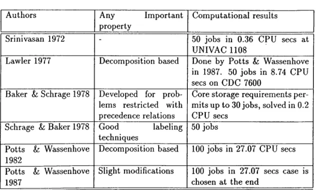
There are many dynamic programming algorithms. Srinivasan 1972 [33], Lawler 1977 [16], Schräge and Baker in 1978 [4, 29] Potts and Wassenhove in 1982 and 1987 [23, 25] are the main ones. The table 2.1 summarizes their results.

The algorithm of Lawler [16] is a pseudopolynomial time algorithm which evaluates all possible decompositions via dynamic programming. The author did not give any computational results but later Potts and Wcissenhove [23] made a computational study of this algorithm. The algorithm could not go further than 50 jobs. Lawler later developed a fully polynomial approximation scheme for his algorithm [17]. The bound of 0{n^P) is transformed to 0{n7 fe) with some manipulations

Authors Any property

Important Computational results

Srinivasan 1972 50 jobs in 0.36 CPU secs at

UNIVAC 1108

Lawler 1977 Decomposition based Done by Potts & Wassenhove

in 1987. 50 jobs in 8.74 CPU secs on CDC 7600

Baker L· Schräge 1978 Developed for prob­

lems restricted with precedence relations

Core storage requirements per­ mits up to 30 jobs, solved in 0.2 CPU secs

Schräge & Baker 1978 Good

techniques

labeling 50 jobs

Potts & Wassenhove 1982

Decomposition based 100 jobs in 27.07 CPU secs

Potts L· Wassenhove 1987

Slight modifications 100 jobs in 27.07 secs case is

chosen at the end Table 2.1; Table of Dynamic Programming Based Exaict Algorithms

In 1978, Baker and Schräge gave two algorithms on this topic. These algorithms are the best known dynamic programming algorithms and have been used by many subsequent researchers. The first one [4] is for problems in which jobs have precedence restrictions. The authors give an approach which can also be used for problems with no precedence restrictions. The authors also give importance to labeling of the sets.

The second paper of Schräge and Baker [29] works on better labeling techniques than the one they proposed in their previous paper. They work out a good algorithm for labeling.

Both algorithms have low CPU time and the core storage permitted handling as many as 50 jobs which are solved in less time than any branch and bound algorithm. The technique given in the second paper is even better than the one based on the chain structure because of the improved labeling. With this algorithm it becomes easier to retrieve the sets when they are needed. This / dynamic programming algorithm is used as a subroutine by some subsequent researchers.

In 1987, Potts and Wassenhove [25] proposed a method which makes some modifications on the dynamic programming algorithms of Lawler and then of Schräge & Baker’s. Their decomposition theorem is applied to the problem in hand until it can be solved by the dynamic programming algorithm of Schräge & Baker. Then, they made some modifications such as using El- magraby’s lemma [10] in branching, using a technique which prevented solving the same problem more than once, and recognizing easily solvable cases like the ones giving SPT optimum or EDD optimum, before attempting to solve the entire set. With these kinds of modifications, the authors managed to solve 100 jobs in less time than they did before. The final step they reach in this study is the best known exact algorithm. It solves 100 jobs in 27.07 seconds on the average on a CDC 7600 computer. The code is in FORTRAN IV.

2.2.2

B ranch and B ound A lgorith m s

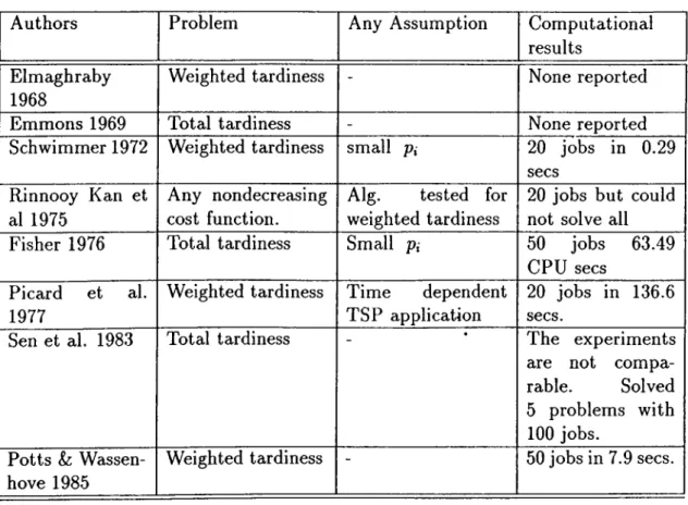
Branch and bound algorithms appeared with the development of theorems that give precedence relations. The first branch and bound algorithm which is based on precedence relations is developed by Elmagrabhy in 1968 [10] and by Emmons in 1969 [11]. Then Schwimmer in 1972 [30], Rinnooy Kan et al. in 1975 [28], Fisher in 1976 [12], Picard and Queyranne in 1978 [21] , Potts Wassenhove in 1985 [24] are the other studies which find an optimum via a branch & bound algorithm. The table 2.2 summarizes the state of the art on branch and bound.

CHAPTER 2. LITERATURE REVIEW 9

In 1976, Fisher [12] developed the best known branch and bound al­ gorithm in terms of the tightness of the lower bound used. He considers the single machine cis posing a constraint on the feasible set of the problem. He performed a Lagrangean relaxation on that constraint and the solution of the relaxed problem gave a lower bound for the initial one. The branch and bound algorithm is based on backwards scheduling with depth first search. Nodes cor­ respond to the set of scheduled jobs up to that time. Begin branching by the possible set of last jobs (known by the use of Emmons’ theorems) and apply depth first search by taking into account the precedence relations (resulting

from Emmons theorems) until fathoming occurs. The fathoming criteria are: i) an initial solution for the problem is first calculated with any heuristic. Use Caroll’s heuristic [5] which is a construction heuristic based on Emmons theo­ rems. At each node the calculated lower bound is compared with the solution of the heuristic and if the lower bound is greater than the total tardiness of the solution, then the node is fathomed.

ii) if the Lagrangean resulted in an optimal solution then the node is fathomed. You have the solution.

iii) if for any two different nodes, the nodes contain the same set of scheduled jobs but have different costs, then the one with higher cost is fathomed (fathom with respect to dominance criteria):

This algorithm can solve up to 50 jobs in reasonable time but it works with small p,· only since the solution to the Lagrangean is obtained in 0{n^Pavg) wherc pavg Is the average processing time. The algorithm can solve 50 job problems and only if jobs have small process times.

The algorithm of Potts and Wassenhove [24] is the fastest one among the known branch &: bound algorithms. Their algorithm is again based on backwards scheduling with depth first search. They also calculate a lower bound for each node. Their lower bound is easy to calculate, is not as good as Fisher’s, but not bad either. In calculating the lower bound they relax the problem so that the resulting problem becomes the minimization of the total completion times. The method is successful up to 50 jobs for the weighted case.

CHAPTER 2. LITERATURE REVIEW 11

Authors Problem Any Assumption Computational

results Elmaghraby

1968

Weighted tardiness None reported

Emmons 1969 Total tardiness None reported

Schwimmer 1972 Weighted tardiness small Pi 20 jobs in 0.29

secs Rinnooy Kan et

al 1975

Any nondecreasing cost function.

Alg. tested for

weighted tardiness

20 jobs but could not solve all

Fisher 1976 Total tardiness Small Pi 50 jobs

CPU secs

63.49

Picard et al.

1977

Weighted tardiness Time dependent

TSP application

20 jobs in 136.6 secs.

Sen et al. 1983 Total tardiness The experiments

are not compa­

rable. Solved

5 problems with 100 jobs.

Potts & Wassen- hove 1985

Weighted tardiness 50 jobs in 7.9 secs.

Table 2.2: Table of Branch Sz Bound Algorithms

2.3

HEURISTICS

The research after 1990, at which time the NP - Completeness is proved, fo­ cused mainly on finding good heuristics. There were studies on heuristics before that time also, but those were mainly in construction type heuristics which may help in upper bounding. In construction heuristics, the schedule is built from scratch by fixing the position of one job at each step. Caroll 1965 [5], Wilkerson and Irwin 1971 [36], Morton and Rachamadugu in 1982 [20], Baker and Bartrand [1] have construction heuristics for the problem. The Wilkerson & Irwin heuristic is in fact a combination of a construction plus some improvement heuristic.

Different types of improvement heuristics began to appear after 1990. Potts and Van Wassenhove in 1991 [26], Lowe et al in 1991 [6] are among those studies. The table 2.3 summarizes existing heuristics in the literature.

Authors Name of heuristic

Any Property Complexity

Caroll 1965 COVERT Construction O(n^)

Morton L·

Rachamadugu 1982

Apparent Urgency

Construction O(n^)

Baker ¿z Bartrand Modified

Due Date

Construction 0{nlogn)

Wilkerson & Irwin

1971 WI Construction Interchange plus Potts L· Wassenhove 1991 Decomposition incorporated with any heuristic

Lowe et al. 1991 Relaxing Emmons theorems

and solving with dynamic programming of Schräge and Baker in sets.

Fry et al. 1989 API 9 different interchanges. Bet­

ter than WI Holsenback & Russel

1992

Construction. Very simple,

even hand calculation is pos­ sible for n < 20 Better than API

O(n^)

Panwalkar et al. 1993 PSK Construction. Best known

Table 2.3: Table for the heuristics

Any of the scheduling rules can be accompanied with interchange heuristics. That is, the resultant schedule of any of the above heuristics can be put into local search heuristics. In 1990, Chang et al. [7] analyzed many types of local search heuristics and derived the worst case behavior for them. They analyzed four main local search heuristics:

ADJ : Adjacent Interchange - Only interchanging a pair of two adjacent jobs K - INT : K - Interchange, Interchanging any pair of jobs at most k times successively

B - S : Backwards Shift, Moving one of the jobs backwards.

G - S : General Shift, Moving one of the jobs forwards or backwards.

They defined a local search heuristic to be any method that starts with an initial sequence and searches for another permutation of the jobs which results in less tardiness.

CHAPTER 2. LITERATURE REVIEW 13

The authors found out that for n > 4 , in the worst Ccise, the first two

interchange based heuristics, ADJ and K - INT can have arbitrarily large (may be oo) relative error (the relative error is defined as the ratio of the worst local optimum value to the global optimum). The authors also showed that shift based heuristics, B - S and G - S, have finite relative error in the worst case.

Another heuristic is developed by Fry et al. [14] in 1989 which is based on adjacent pairwise interchanges (API). Since adjacent pairwise interchanges can only result in a local optimum, the authors tried to evaluate different solutions and select the best at the end. The initial sequence in starting the local search effects the solution, so the authors tried three different initial sequences, namely, SPT, EDD, and SLK (Smallest Slack Rule) which schedules jobs in nondecreasing order of C,· — d,· where Ci denotes the completion time of job i. The interchange strategy will also affect the result. The authors matched the three initial sequences with three different interchange strategies so there were nine different solutions for each problem. At the end they select the best of these nine solutions as the result of the API heuristic.

Most recently, in 1992, Holsenback and Russel [15] developed another heuristic. In their review of the literature the authors say that the API heuris­ tic of Fry et al. (explained before) was the best of the existing heuristics in terms of solution quality where solution quality is defined as the mean per­ centage deviation of the heuristic from the optimum. The authors claim that they developed a better one, both in solution quality and running time. The heuristic starts with an EDD schedule and tries to improve the sequence. The

reducible tardiness criterion is used in the improvement. Any job which has

tardiness greater than its processing time ( Tk> Pk where Tk is the tardiness of job k) is said to have reducible tardiness. In the algorithm, inspecting jobs

from the last to first, the first job having reducible tardiness, say job is

identified. Given k, the predecessors of job k (in the current sequence) are inspected in the order A: — 1, ¿ —2,.. until the first job is found whose movement to position A: -|- 1 (i.e. right after k ) improves the total tardiness. With this movement the tail end of the sequence from positions A: -|-1 up to n is fixed. For the remaining jobs (i.e. jobs 1,...,A:) the same procedure is applied. The

algorithm continues until no job with reducible tardiness can be found. The complexity of the algorithm is O(n^). The important property of this heuristic is its easiness. Even hand calculation is possible with this heuristic for n < 20.

In 1993, a better heuristic is developed by Panwalkar et al. [22]. This heuristic is the best known one for the single machine total tardiness problem, both in solution time and in solution quality. The authors compared their heuristic with that of Wilkerson and Irwin, Holsenback and Russel and the API method of Fry et al. and showed, by making many experiments, that their heuristic is better than all of the others. The algorithm makes n passes

from left to right and at the pass it picks one job and schedules it to the

k^^ position. Each pass starts with the smallest job in hand, calls it the active

job, and tries to fix this job by considering some inequalities or changes the active job.

Chapter 3

^-SEQUENCE and

DECOMPOSITION

THEOREMS

In this chapter we analyze the earlier results from the literature which we use in our algorithms. The first section gives Emmons theorems [11]. The second section is on the ^-Sequence of Tansel & Sabuncuoglu [34] and the third section gives the decomposition theorems of Lawler [16], Potts & Wcissenhove [23], and Tansel & Sabuncuoglu [34]

3.1

Emmons’ theorems

The theorems of Emmons are the basic building blocks in the scheduling theory of total tardiness. Nearly all subsequent researchers used these theorems in their studies.

To state the theorems assume jobs are indexed according to the nonde­ creasing processing times by breaking ties with nondecreasing due dates. That is j < k implies pj < pk or pj = pk and dj < dk. This indexing will

be referred to as the SPT (Shortest Processing Time) indexing. Throughout the thesis, we use SPT indexing unless otherwise mentioned and we denote

P* =

EieJPi-We define a subset Bj of J to be a before-set of j if there exists an optimal sequence in which every job in Bj precedes job j . Similarly, a subset

Aj of J is defined to be an after-set of job j if there is an optimal sequence

in which every job in Aj succeeds job j. We also define Ak = {f : i ^ Ak\ Theorem 1 For j < k ii Bk is a before set of job k and

dj < max Pi+Pk , dk} ieBk

then Bk U {^'} is also a before set of job k (i.e there exist an optimal sequence in which every job in Bk as well as job j precede job k).

Theorem 2 For j < A; if Bk and Ak are before and after sets of job k,

respectively, and ¿) dj > maxlY^i^B^ Pi + Pit, dk}

ii) ¿ j + P j > Pi

then Ak U } is also an after set of job k.

Theorem 3 For ; < A: if A j is an after set of job j and

dk > Pi i 6 A j

then A j U {A:} is also an after set of job j.

We use the notation j <— A: to mean there exist an optimal sequence in which job j precedes job k.

The first theorem gives the conditions for a smaller job being a pre­ decessor of a larger one whereas the second theorem is for a larger job being a predecessor of a smaller one. Repeated use of the theorems will give many relations and those relations will form succesively expanding before-sets and after-sets of each job. That is once we find j is before A; we insert job j in

the most recent before set of job k and insert job k in the most recent after set of j .

The proofs of the theorems are based on either interchanging two jobs or moving one job to a later position. While making these movements or interchanges, say for proving j *— k, the author assumes the opposite ( that is, job k is placed before job j in a sequence) and shows that the tardiness of the sequence will not get worse by interchanging jobs j and k or by moving job j right after job k. The following discussion give the main ideas that lead to Emmons‘ theorems.

Let j < k and suppose we have a sequence S in hand with job k

placed before job j. Jobs j and may or may not be adjacent. Now we study

the changes in the tardiness function when we interchange jobs j and k and we derive conditions under which the interchange decreases the total tardiness.

Let the sequence after interchanging job j and job k be S.

CHAPTER 3. 0 -SEQUENCE AND DECOMPOSITION THEOREMS 17

middle set middle set

w

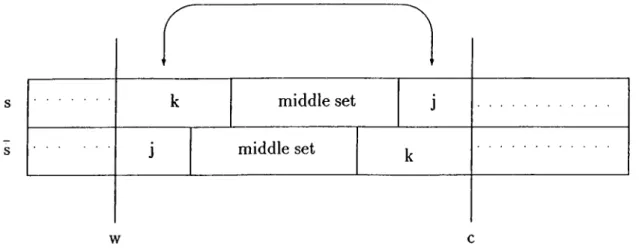
Figure 3.1: Illustration for an interchange

Let W be the waiting time of job k in S and C be the completion time of job j in S. So only the jobs whose completion times are between W and C are alfected from this movement. We call these jobs as the middle set and denote the tardiness of these jobs in sequence S by T{ middle set ). If we define T{S) to be the tardiness of sequence S and T{S) to be tardiness

of S, we have

T{S) = maa:{0, VK + pjt — + maa:{0, C — dj} + T(middle set ) T K

T{S) = max{0, W + pj — dj} + max{0, C — dk) + T(middle set ) + K

where K is the total tardiness of the unaffected jobs.

Since j < k implies pj < pk the tardiness of the middle set can not get worse. The change in tardiness is

A = T{S) - T{S)

> m ax{0 ,W + p k—dk}-{-max{0^ C — dj} — max{0, W-\-pj—d j} —max{0, C — dk}

where the inequality follows from T{ middle set )—T( middle set ) > 0. Define the right hand side of the inequality to be A.

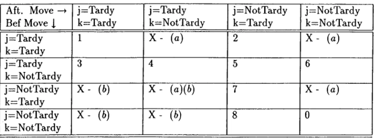
We consider 16 cases corresponding to two possibilities for each max- imand. The following table identifies the 16 possibilities.

Aft. Move Bef Move J. j=Tardy k=Tardy j=Tardy k=NotTardy j=NotTardy k=Tardy j=NotTardy k=NotTardy j=Tardy k=Tardy 1 _{X - (o)} 2 X - (a) j=Tardy k=NotTardy 3 4 5 6 j=NotTardy k=Tardy X - (6) X - (a)(4) 7 X - (a) j=N ot Tardy k=NotTardy X - (i) X - (4) 8 0

Table 3.1: Table for tardiness changes after an interchange

In the table, we marked some of the cells by X to indicate that the cell will not arise. For example, for X{a) , the condition of the cells mean job k is tardy in S and it becomes not tardy in S which is impossible. Also for X{b), the condition of the cells show job j is not tardy in S whereas it becomes tardy in S which is impossible.

Now let us see the change in the tardiness for each of the cell in the table above. We look at A.

Cell 1 A = [W pk — dk -\- C — dj) — (W + Pj — dj C ~ dk) = Pk ~ Pj ^ 0 since j < k

Cell 2 A = { W - h p k - d k - l · C - d J ) - { C - d k ) = W - \- p k - d^

Cell 3 A = (C — dj) — (VK Apj — dj -\-C — dk) — dk — ]V — pj ^ dk — W — pk ^ 0

since k is not tardy in S in this cell so that dk > W

pk-Cell 4 A = (C - dj) - {W A pj ~ dj) C - W - pj > p k > 0

Cell 5 A

= (C

4 ) = 4 - 4

Cell 6 A = ( C - 4 ) > 0

Cell 7 A = {W + Pk — dk) — {C — dk) = W A p k — C < 0 since C > W A p k A p j C ells A = - ( ( 7 - 4 ) < 0

Let us summarize the results of A in the next table

CHAPTER 3. 0 -SEQUENCE AND DECOMPOSITION THEOREMS 19

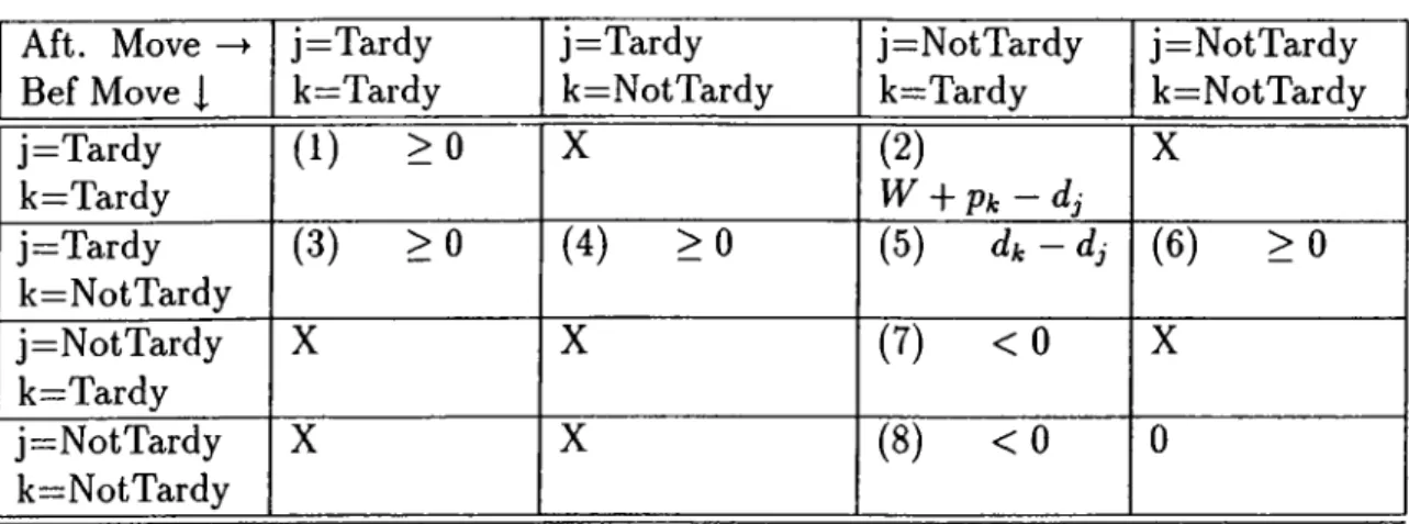
Aft. Move —>■ Bef Move J. j=Tardy k=Tardy j=Tardy k=NotTardy j=NotTardy k=Tardy j=NotTardy k=NotTardy j=Tardy k=Tardy ( 1) > 0 X (2) W A P k - dj X j=Tardy k=NotTardy (3) > 0 (4) > 0 (5) die dj (6) > 0 j=NotTardy k=Tardy X X (7) < 0 X j=NotTardy k=NotTardy X X (8) < 0 0

Table 3.2: Tardiness changes after an interchange

In order for the interchange to improve tardiness we want A > 0 for all of the cells. Since there are some cells with A < 0 and others where A can be negative, zero or positive we need to impose conditions to avoid them.

We only need to look at the cells 2, 5, 7 and 8. Since we have

4

4

of the cells , let us first impose the condition 4 > 4 ·

Cell 2 W A Pk — dj =‘1 Since we use

4

W A P k - d . j > W A Pk dk ^ 0 since k is tardy in S and W > 0

For the cells 7 and 8 we need conditions for avoiding them. Let us see if dt > dj works here or not

Cell 7 In this cell job j is not tardy in both sequences and job k is tardy in both of them.

k _j

j 1₁

--- 1--- --- 1---¡k

w

Figure 3.2: The conditions of cell 7

So if dk > dj this case will not arise.

Cell 8 is similar to cell 7 and the condition dk > dj avoids this cell also. So if pj < pk and dj < dk then the sequence S has no more tardiness than S and so we can say that in some optimal sequence job j will be scheduled before job k{ otherwise, interchanging those jobs will not increase the tardiness).

If we define P{Bk) as the total process times of the jobs in the before­ set of job fe, with similar arguments, A > 0 condition can also be satisfied with P{Bk) +Pk > dj condition.

So for Pj < Pk either dj < dk or dj < P{Bk) -f Pk is needed to have an improvable interchange. Hence, if pj < pk and dj < max{dk, P{Bk) -1- Pk} then job j is before job k in some optimal sequence. This is the first theorem of Emmons.

CHAPTER 3. 13-SEQUENCE AND DECOMPOSITION THEOREMS 21

Now suppose we know that the above inequality is not satisfied for jobs

j and k. Since we cannot say that j is before k in some optimal sequence, let

us see if we can say that k is before j in some optimal sequence. This time put j before fc in a sequence S and form the second sequence S by moving job j to the position right after job k. The figure below will be helpful.

Figure 3.3: Illustration for a movement Again, the total tardiness for S and S are

T{S) = maa;{0, W pj - dj) + ma x{0, C - dk} + T{ middle set ) + K T(S) = max{0, C — dj) + max{0, C — pj — djt} + T{ middle set ) + K

We assume that the first theorem is violated; that is, assume

Pj < Pk ,dj > max{dk,P{Bk) + Pk}

The table below illustrates the cases to consider. Since, now we are moving job j right after job k the table has a slightly different form.

Aft. Move - Bef Move J. j=Tardy k=Tardy j=Tardy k=NotTardy j=NotTardy k=Tardy j=NotTardy k=NotTardy j=Tardy k=Tardy 1 2 X (c) X (a) X (c) j=Tardy k=NotTardy

X (i.) 3 X (c) X (a)((.) X (a)

j=N ot Tardy k=Tardy j=N ot Tardy

k=NotTardy

X (6) 8 X (c) X (b)

Table 3.3: Table for tardiness changes after a movement

The X’s are again denoting the cases which cannot arise. X (a) cannot occur because if job j is tardy before, it will continue to be tardy; X (6) cannot occur because if job k was not tardy before, then it will continue to be not tardy, and finally X (c) cannot occur due to the condition dj >

max{dk, P{Bk) + Pk) >

dk-The table below summarizes the results found for the remaining cases. Aft. Move —> Bef Move J, j=Tardy k=Tardy j=Tardy k=NotTardy j=NotTardy k=Tardy j=NotTardy k=NotTardy j=Tardy k=Tardy (1) W +2p j - C X X X j=Tardy k=NotTardy X X X X j=N ot Tardy k=Tardy (4) Pi + dj — C (5) > 0 (6) > 0 (7) > 0 j=NotTardy k=Not Tardy X X X 0

CHAPTER 3. j3-SEQUENCE AND DECOMPOSITION THEOREMS 23

We again want to have A > 0 for all cells so we need to analyze cases 1 and 4. Let Ak be the after set of job k and let Ak = J - Ak- Then we can

say that C < P{Ak) and P{Ak) > W + pj -\-pk- Suppose dj pj > P{Ak)

then dj + Pj > P{Ak) > W + Pj + Pit and so dj > W + pk > W + pj. Then j was not tardy before which eliminates cell 1.

For cell 4, since we assume pj + dj > P{Ak) and since ^(^4*) > C this cell is satisfied by the condition imposed.

So for Pj < pk if dj > max{dk,P{Bk) +Pfc} and pj + dj > P{Ak) then job k is before job j in some optimal sequence, and this is the second theorem of Emmons.

In 1976, Fisher [12] relaxed these theorems, by first removing j < k condition from the third theorem and removing one of the maximands from part (¿) of the second theorem. That is (¿) can be taken as dj >

dk-Here it will be better to give the geometric view of Tansel L· Sabun- cuoglu [34]. With their point of view theorems of Emmons become really easy to handle. Especially their look at theorem 1 is worth mentioning. De­

fine Ek = 12ieBk P‘ "b be the earliest completion time of job i and

Lk = J2ieAk P* be the latest completion time of it. Recall that Bk and Ak

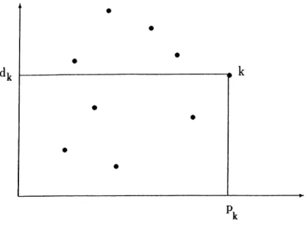
are the before and after sets of job k and Ak = J — Ak . Plot the data on a graph with each data point being represented by (p^, max{dk, Ek}) W k G J.

Initially, no relation is known, and Ek = Pk- Ek becomes larger when we

find relations. Each job k has an enclosing rectangle which is defined by the following points cis the corners :

(0,0), (pit, 0), (0, max{dk, Ek}), {pk, max{dk, Ek})

A point (pj, m a x { E j , dj}) is said to be in the enclosing rectangle of job

k if the point is in the interior or on the boundary of the enclosing rectangle of

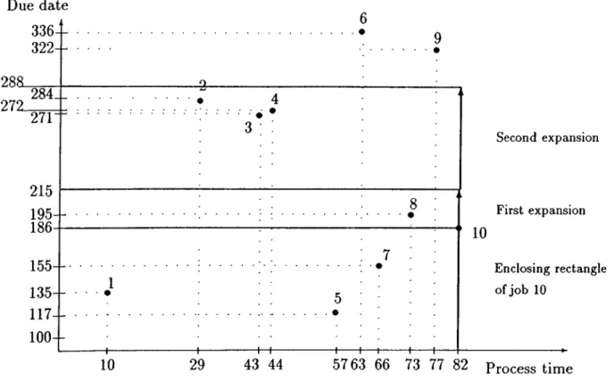
job k. An equivalent statement of Theorem 1 of Emmons is as follows : With SPT indexing, if the point corresponding to job j is in the enclosing rectangle of k then job j is before job k in some optimal sequence. The figure 3.4 illustrates the idea.

Due date 3363 2 2 -288_ 272.284. _ 271 215 195 186 155- 135- 117-100 -10 4 6 9 8 -H—t- H----h -t----h Second expansion First expansion 10 Enclosing rectangle of job 10 29 43 44 5763 66 73 77 82 Process time

Figure 3.4: Graph for the illustration of enclosing rectangle

For example in Figure 3.4, initially Bio —

0

1, 5, 7 are in the enclosing rectangle of job 10, Bio now expands to {1,5,7} and Eio becomes 82 + 10 + 57 + 66 = 215. The enclosing rectangle of job 10 expands vertically indicated by the arrow in the figure and now job 8 is also in the rectangle. Now Bio = {1,5,7,8} and Eio = 215 + 73 = 288 and jobs 2, 3, 4 fall in the enclosing rectangle of job 10. With these rectangular movements, the relations become very easy to handle.

3.2

^-sequence

With the repeated use of Emmons’ theorems, a new sequence, called the /9-Sequence, is developed by Tansel L· Sabuncuoglu. The /^-Sequence happens to be an optimal sequence under certain conditions. Let us give some definitions

CHAPTER 3. ¡3-SEQUENCE AND DECOMPOSITION THEOREMS 25

first.

For any job j four different sets are constructed. These are referred to as right-down, left-down, right-up, and left-up sets of job j , denoted by

R D j , L D j , R U j , L U j , respectively. Let a,· = m a x { p i, d i) Vi.

The sets are defined as

R D j = {i : i ^ J,i > j , and a, < ctj} L D j = {i : i E J,i < j, and or, < aj} R U j = {i : i ^ J,i > j, and a,· > ay} L U j = { i : i E J,i < ji, and a, > ay)

For example, for job 7 in Figure 3.4 we have

LDj =

{

,

},

=

,

(

,

,

,

},

{

,

,

}

In fact L D j is the set of jobs in the enclosing rectangle of job j.

The ^-Sequence is generated by using the earliest completion times of the jobs resulting from the before-sets. While forming the before-sets the left-down and right-down sets are used. The usage of the left-down set corre­ sponds to the use of Theorem 1 of Emmons in finding the before-sets. That is, for i G LDj, the relation i <— j is available from Tansel & Sabuncuoglu’s interpretation of Theorem 1. The use of right-down set corresponds to the use of Theorem 2 of Emmons. For i € RDj , a job being in RDj means that

Pj < Pi and max{dj, Ej} > di which are the first two requirements of theorem

2 of Emmons. So for any i G RDj, if py -f dj > Li then i *— j can be concluded.

We form the earliest completion time E j of job j in two steps after

initialisation:

Initial: Assign ^ j = m a x { p j , d j ) ' i j and form L D j , R D j with respect to point

(ft.ft)V j.

Step 1 - For each newly included k in the most recent L D j , we increment E j

with respect to point (pj,/3j).

Step 2 - For each newly included k in the most recent R D j , if Pj-\-^j > Lk then

we increment E j by pjt while decreasing Lk by p j, assign = m a x { d j ^ E j )

and redefine R D j with respect to point (p j,^ j).

These steps are repeated as many times as possible. Termination occurs when no more incrementation can be done.

The /^-Sequence is the sequence of the jobs when we order them in nondecreasing order of their final ^ values with ties broken by nondecreasing order of process times. Let Dj{^) denote the jobs sequenced before job j in the ^-sequence and RDj{l3) be the most recent right down set of job j at termination of steps 1 and 2.

The ¿^-Theorem of Tansel & Sabuncuoglu is :

Theorem If ¡3j > P { D j{ /3)) W j with R D j{ ^ ) ^ 0 then the /^-Sequence is

optimal for the original problem.

If (¿) RDj{^) = 0 or (it) RDj{l3) ^ 0 and Pj > P{Dj{^)), then we say job j passes the /?-test, otherwise we say job j fails the /3-test. Note that failure occurs if and only if RDj{^) ^ 0 and ^j < P{Dj{0)). If all jobs pass then the y3-Sequence is optimal. Otherwise nothing can be said about the optimum sequence. That is, a failed ;0-Sequence may or may not be optimal.

Let me give an example here to illustrate the idea.

Ex 1 Suppose we have 7 jobs to schedule. The process time and due dates are shown in the table below. Applying Emmons’ theorem to find precedence relations between job pairs we find earliest completion times for the jobs. The resultant early completion times of those 7 jobs are below:

CHAPTER 3. /3-SEQUENCE AND DECOMPOSITION THEOREMS 27

Job No Process time DueDate Final Ei's Final /9,’s

1 19 246 19 246 2 26 250 105 250 3 60 246 79 246 4 63 275 168 275 5 64 309 319 319 6 77 328 396 396 7 87 280 255 280

The beta sequence is 1 3 2 4 7 5 6 For job 1 down set total is zero (pcisses).

For job 3 down set total is p\ = 19 and if /?3 = 246 > pi = 19 (passes) For job 2 ^2 = 250 > 19 + 60 = 79 (passes)

For job 4 275 > 79 + p2 = 105 (passes)

For job 7 280 > 105 + P4 = 168 (passes)

For job 5 319 > 168 + pr = 255 (passes)

For job 6 396 > 255 + ps = 319 (passes)

So the /9-Sequence is optimal.

3.3 Decomposition theorems

The decomposition idea, first developed by Lawler [16], is the next tool that we use in our algorithms. Decomposing means handling each part alone, inde­ pendent of the other. So the number of jobs in hand at a time decreases. The problem is that the decomposition theorem of Lawler results in many possi­ ble alternative decompositions axid there is no a priori information on which particular decomposition(s) yields an optimal sequence.

The decomposition theorem of Lawler is also applicable to weighted tardiness problem. For the decomposition principle to apply, jobs are assumed to be agreeably weighted] that is, if p, < pj then tn, > wj. For the total

tardiness problem since all W{ = 1 this condition passes immediately. Begin

with reindexing the jobs in EDD order, i.e d\ < < dz < ... < d„ and

break ties by nondecreasing process times. Let job k be the largest indexed job with the largest processing time. The decomposition theorem states that

there exists an integer Q < 8 < n — k , such that there is an optimal

sequence in which k is preceded by all jobs j '■ j < k E 8 and followed by all

jobs j : j > k 8. So using this principle the problem can be decomposed

into subproblems without losing from optimality. That is, there is an optimum

sequence which is in the following order according to 8:

i) l , 2 , 3 , . . . , k - l , k + l , . . . , k-\-8

ii) k

Hi) fc + (5+l,A: + <5 + 2, ...,n

In fact, this theorem can be seen from theorem 1 of Emmons if we look at it from the view of Tansel & Sabuncuoglu. Since k is taken to be the largest job, there will be no point in the right side of job k in the graph. The figure below will be helpful in the explanations.

The jobs in the enclosing rectangle of job k will be sequenced before job k and for the ones above the rectangle, nothing can be said in terms of theorem 1. The decomposition theorem of Lawler uses this idea. The jobs in the enclosing rectangle of job k are the ones which have less due date than that of job k. Since we are using the EDD indexing, then those jobs will be the ones from 1 to k - 1. So in some optimal sequence, job k will be sequenced after the jobs which have less due date than itself, regardless of how the jobs in the enclosing rectangle are sequenced. The jobs which have d, < djt will be surely before job k. The rest of the jobs should be checked in both before

k and after k. So there are many possible decompositions, in terms of this

decomposition theorem.

Then Potts and Wassenhove [23] worked on the theorem and decreased the search space. In order to understand what is going on let us drive the conditions from scratch. We are trying to find places A: + d to which moving

job k is not profitable. That is, we assume job k is at place k S and then

derive conditions for which moving job k forwards or backwards decreases the

tardiness . Then we conclude that with those conditions, the place k 6 will

not be an alternative for job k.

We know that pk > Pi V i and

dk < dk+i < djt+2 < ... < dk+s-i < dfc+5 < ... < d«.

CHAPTER 3. 0-SEQUENCE AND DECOMPOSITION THEOREMS 29

Let us first look at the case of forward movement from place A: + <5. Job k is at place A: + ^ and we derive the conditions under which moving k from A; + d will be profitable. The figure 3.6 shows the sequences, S before the movement and the sequence S after the movement.

Figure 3.6: Illustration of a forward movement

The table below illustrates the idea. Let A = T{S) — T{S) and

let j = k ~I· 6 1. After Move —> Bef Move 1 k=Tardy j=Tardy k=Tardy j=N Tardy k=NTardy j=Tardy k=NTardy j=NTardy k=Tardy j=Tardy Pk - P j > 0 (2) W + p t - d , X X k=Tardy j=NTardy X (3) < 0 X X k=NTardy j=Tardy X (5) dk - d j < Q X X k=NTardy j=N Tardy X (8) < 0 X 0

Table 3.5: Tardiness changes resulting from the forward movement We are trying to find conditions for which moving job k is profitable, so we want A > 0. So we need to eliminate cases 3, 5 and 8 while trying to

make cell 2 > 0. If we impose W pk — dk+s+i > 0 then dk+s+i < W + pjt

and so job ^ 5 + 1 is tardy in the sequence S which eliminates cases 3 and

8 immediately.

For case 5: Since dk+s+i < W + pjt < where the last inequality

follows from job k ’s being not tardy in S and since dk < dk+s+i this case is also eliminated.

CHAPTER 3. 0-SEQUENCE AND DECOMPOSITION THEOREMS 31

So if

i=k-\-5 i=k-\-6

dk+s+i < W + P k < ^ P i - P k + P k = ^ Pi ioT 6 < n - k

i = l .= 1

then job k will not stay at place k -P S .

Now, let us derive a similar relation from the backwards movement of the job k assumed to stay at place ^ + i. The figure below will show the sequence before the move, S, and after the move S.

Figure 3.7: Illustration of a backward movement The table below shows the resultant A = T(S ) — T(S) After Move Bef Move | k=Tardy k+ ¿=Tardy k=Tardy k+ i=N Tardy k=NTardy k+ ¿=Tardy k=NTardy k+ ¿=NTardy k=Tardy k+ ¿=Tardy (1) Pk+S — Pk < 0 X (2)X X k=Tardy k+ ¿=NTardy

(3)

₍₅₎

Table 3.6: Tardiness changes resulting from the backward movement

Since we want the cells to be > 0 we want to eliminate cell 1 and want cell 3 to have A > 0 . Try the condition of cell 3 which is dk+s ^ W +pjt·

Since

dk+s > W + p k > W + pk+s

then job k + 6 is not tardy in sequence S which eliminates cell 1 while causing

cell 3 to be > 0 . But this time we need to pay attention to the equality case since we moved the larger job backwards. Suppose dk+s = kF + pk- The corollary 2.3 of Emmons states that

if jobs j and k with j < k are to occur consecutively after a waiting time W

then they should be sequenced according to the rule

j *— k if and only if dj < m a x { W + pk,dk}.

We will see if dk+s = VT + p;t is feasible for our aim or not by checking

this corollory. For our case k + 6 < k. If dk+s < m a x { W + then

k -\· S *— k will be concluded which contradict with our aim.

In cell 3 k is tardy in S and S and so dk < W -\-pk. Then the maximand in

the inequality becomes W A Pk and since

dk+s - W Apk = m a x { W + pk,dk}

then we conclude that k A S *— k.

So, the condition needed here is to have

i = k + S

dk+s > W A p k = X] Pi for <5 > 0.

¿=1

If this is so, then job k will not stay at place k A S.

Finally, if or dk+6> £ Pi for (5 > 0 (1) t= l dk+s+i < X) Pi for 5 < n - A; (2) i= l

then job k will not go to place k A S.

So, if

dk+6 < S P i < dk+s-i - Pk+s for 0 < 6 < n - k

CHAPTER 3. /3-SEQUENCE AND DECOMPOSITION THEOREMS 33

then place k 6 will be an alternative for job k.

The inequality (2) is not valid for 6 = n — k case since at S = n — k

the place fc + i + l = n + l will be meaningless. So for 6 = n — k only the

condition (1) will be valid, that is, the job will go to place n if dn < P i

-For condition (1) , ^ = 0 is meaningless since we are trying to move job k

at place k 6 backward, with 6 = 0 the movement will be meaningless. So

for i = 0 , only the condition(2) will be used, that is, the job will stay at its

original place if djt+i > 5Z|=i Pi

Now let us state the decomposition theorem of Potts &: Wassenhove in the formal form . First reindex in FDD. For any k,l € J a problem is said to

decompose with job k in position I if there exist an optimal sequence in which

jobs 1,..., A: — 1, A: + 1 ,...,/ are sequenced before job and jobs / + 1 , ...,n are

sequenced after job k .

Theorem(Potts L · Wassenhove (1982)) The problem decomposes

with job k in position / for some / satisfying one of the below conditions:

(i) I = k

i=l

and

E

•=i

t = / - l

(ii) I = k + 1, ...,n — 1 and d/ < ^ p,· < d/+i — pi

«■=1 /-1

(Hi) I = n and > d\

»=1

The theorem says that by moving job k to the position we decom­

pose the problem into two sets. The ones in the first / —1 positions forming the before set and the rest forming the after set. Both can be solved independent of the other by taking the ready times for the after set into consideration.

It would be better to show the decomposition theorem on an example here.

E x 2 Suppose we have 16 jobs to be scheduled. The processing times and the due dates are below:

Job No Proc. time DueDate

1 85 241 2 15 246 3 77 292 4 23 325 5 15 385 6 41 390 7 43 417 8 35 418 9 14 432 10 66 432 11 42 440 12 1 456 13 49 475 14 15 490 15 59 506 16 26 519

Since the theorem is based on an EDD schedule we need to have EDD indexed jobs. Our current data satisfies it. The job with the largest process time is job 1. So places between 1 to n will be searched.

/ = 1 if Ei=} Pi = 85 < ¿2 = 246 PASS

7 = 2 if ¿2 < E i } Pi = 85 FAIL

/ = 3 ifd 3 = 292 <E;'=?P. = 100- / = 4 if ¿4 = 325 < Ei=? Pi = 177

/ = 5 ifds = 385 = 200

/ = 6,7,8,9,10 and 11 also FAIL

/ = 12 if di2 = 417 < E i=P = 456 and 456 < d n - Pu = 475 - 1

/ = 13 if di3 = 475 < Elii^P.· = 457 FAIL

/ = 14 if ¿14 = 490 < E !=P = 506 and 506 < ¿is - Pi3 = 506 - 49 FAIL

FAIL FAIL

PASS