IZ
M
IR
K
A
T
IP
C
E
L
E
B
I
U
N
IV
E
R
SI
T
Y
J
A
N
U
A
R
Y
2018
NUR
Ç
OB
A
NO
Ğ
LU
M.Sc. THESISCUSTOM DESIGNED OPTICAL TWEEZER FOR TRAPPING YEAST CELLS
Thesis Advisor: Assist. Prof. Aziz KOLKIRAN Nur ÇOBANOĞLU
Department of Nanoscience and Nanotechnology IZMIR KATIP CELEBI UNIVERSITY
GRADUATE SCHOOL OF NATURAL AND APPLIED SCIENCES
JANUARY 2018
IZMIR KATIP CELEBI UNIVERSITY
GRADUATE SCHOOL OF NATURAL AND APPLIED SCIENCES
CUSTOM DESIGNED OPTICAL TWEEZER FOR TRAPPING YEAST CELLS
M.Sc. THESIS Nur ÇOBANOĞLU
(Y150203004)
Thesis Advisor: Assist. Prof. Aziz KOLKIRAN Department of Nanoscience and Nanotechnology
Nanobilim ve Nanoteknoloji Anabilim Dalı
OCAK 2018
İZMİR KÂTİP ÇELEBİ ÜNİVERSİTESİ FEN BİLİMLERİ ENSTİTÜSÜ
ÖZEL YAPIM OPTİK CIMBIZ İLE MAYA HÜCRESİ MANİPÜLASYONU
YÜKSEK LİSANS TEZİ Nur ÇOBANOĞLU
(Y150203004)
v
Thesis Advisor : Assist. Prof. Aziz KOLKIRAN ... Izmir Katip Celebi University
Jury Members : Assist. Prof. Aziz KOLKIRAN ... Izmir Katip Celebi University
Assoc. Prof. Mustafa CAN ... Izmir Katip Celebi University
Prof. Dr. Muzaffer ADAK ... Pamukkale University
Date of Submission : 12.12.2017 Date of Defense : 05.01.2018
Nur ÇOBANOĞLU, a M.Sc. student of IKCU Graduate School Of Natural And Applied Sciences, successfully defended the thesis entitled “CUSTOM DESIGNED OPTICAL TWEEZER FOR TRAPPING YEAST CELLS”, which she prepared after fulfilling the requirements specified in the associated legislations, before the jury whose signatures are below.
vii
ix FOREWORD
This thesis is my final work for completion of master degree at Department of Nanoscience and Nanotechnology in Izmir Katip Celebi University. The goal of the thesis is the development of custom designed optical tweezer in order to trap yeast cells and study the possibility of optical tweezer in biological applications. From beginning to end, all steps of this thesis were under the supervision of Assist. Prof. Aziz Kolkıran.
Firstly, I am grateful to my supervisor, Assist. Prof. Aziz Kolkıran, for his excellent guidiance, valuable and constructive suggestions during my master degree.
In addition, I would like to thank to Erdal Kurt for his supports during my thesis. Finally, I would like to thank my parents, Uğur Çobanoğlu and Nurdan Çobanoglu, and my brother, Can Çobanoğlu, for supporting me and being a source of motivation and inspiration in my life.
xi TABLE OF CONTENTS Page FOREWORD... ix TABLE OF CONTENTS ... xi ABBREVIATIONS ... xiii SYMBOLS ... xv
LIST OF TABLES ... xvii
LIST OF FIGURES ... xix
ABSTRACT ... xxi
ÖZET ... xxiii
1. INTRODUCTION ... 1
1.1 Historical Background of Optical Tweezers ... 2
1.2 Applications of Optical Tweezers ... 4
2. THE BASICS OF THE OPTICAL TWEEZER ... 7
2.1 Physical Principle of Optical Tweezer ... 7
2.1.1 Ray Optics approximation ... 8
2.1.2 Rayleigh approximation ... 9
2.1.3 Generalized Lorenz-Mie theory ... 10
2.2 Trapping Efficiency ... 17
2.3 Detection and Calibration of Optical Forces ... 17
2.3.1 Force detection techniques ... 17
2.3.2 Calibration techniques ... 18
2.3.2.1 Drag force method ... 19
2.3.2.2 Brownian Motion method ... 19
2.3.2.3 Escape force method ... 20
2.3.2.4 Power spectrum method ... 20
2.3.2.5 Step response method ... 21
3. THE BASIC ELEMENTS OF OPTICAL TWEEZER ... 23
3.1 Trapping Optics ... 24
3.1.1 Lasers ... 24
3.1.2 Lenses ... 25
3.1.3 Sending the light through the objective ... 25
3.1.4 Objective ... 25
3.2 Sample manipulation ... 25
3.3 Imaging System ... 26
4. THE ALIGNMENT PROCEDURE ... 27
4.1 Gaussian Beam Optics ... 28
4.1.1 Gaussian beam propagation and ABCD matrices ... 31
5. LASER SETUP ... 35
6. RESULTS ... 43
6.1 Characteristics of Optical Tweezer ... 44
xii
6.1.2 Results for Laser 2 ... 45
6.1.3 Result when both lasers used simultaneously ... 46
6.1.4 Moving polystyrene beads with laser 2 to laser 1 ... 46
6.1.5 Trapping multiple polystyrene beads ... 47
6.1.6 Comparison of lasers ... 48
6.2 Results for Yeast Cells ... 49
6.2.1 Results for laser 1 ... 50
6.2.2 Results for laser 2 ... 52
6.2.3 Trapping multiple particles ... 53
6.2.4 Moving particle between each other ... 54
6.3 Measuring Viscosity ... 55
6.4 Results When Cytoplasmic Medium Was Used ... 55
6.5 Trapping Efficiency of the System ... 58
7. CONCLUSIONS ... 59
REFERENCES ... 61
APPENDICES ... 69
APPENDIX A:ABCD MATLAB CODES FOR GAUSSIAN BEAM PROPAGATION ... 69
xiii ABBREVIATIONS
FWHM : Full Width Half Maximum GLMT : Generalized Lorenz-Mie Theory NA : Numerical Aperture
R : Reflection
T : Transmission
TE : Transverse Electric TM : Transverse Magnetic
xv SYMBOLS
𝒂 : Radius of the bead
an, bn : Wave scattering amplitudes 𝑨𝒏𝒎, 𝑩𝒏𝒎 : Partial wave scattering amplitudes B : Magnetic field
c : Speed of light 𝑪𝒏𝒎, 𝑫
𝒏
𝒎 : Partial wave interior amplitudes
D : Diameter
dobj : Incident beam diameter to objective E : Electric field
𝑬𝟎 : The peak electric field strength fc : Corner frequency
Fg,Fs, FT : Beam confinement parameter f/# : Photographic f number 𝒈𝒏,𝑻𝑬𝒎 , 𝒈
𝒏,𝑻𝑴
𝒎 : Beam shape ccoefficients H : Kinetic energy
I : Intensity of the light k, kx, ky : Stifnesses kb : Boltzmann’s constant N : Number of frames 𝒏𝒑, 𝒏𝒎𝒅 : Refractive indexes 𝒏 : Normal to surface P : Power 𝑷𝒏𝒎 : Legendre function Q : Trapping efficiency
q1, q2 : Parameters of Gaussian beam before and after the optical element r : Position of the beam
𝑹 : Fresnel reflection coefficient R(z) : Radius of curvature
s : Beam confinement parameter 𝑻 : Fresnel transmission coefficient ux, uy : Broomwich potentials
v : Velocity
w0 : Electric field half-width
w0 : Beam waist diameter w(z) : Radius of the beam
wtrap : Trap depth
x : Distance of the bead’s center from trap center zR : Rayleigh range
xvi 𝝍𝒏 : Ricatti-Bessel function 𝜽 : Incident ray angle 𝝋 : Refracted ray angle 𝜁7 : Ricatti-Henkel functions 𝝁 : Viscosity of the medium
g : Drag coefficient
t : Time constant
<x2> : Time-averaged square of the bead’s horizontal displacement from the center of the trap.
<y2> : Time-averaged square of the bead’s vertical displacement from the
xvii LIST OF TABLES
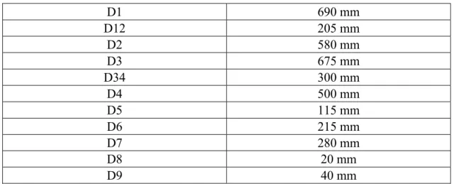
Page Table 5.1 : Distances between optical components. ... 36 Table 5.2 : Power of the beams after optical components. ... 36
xix LIST OF FIGURES
Page Figure 2.1 : Optical forces. Gradient force is shown in red; scattering force is shown
in purple. ... 7
Figure 2.2 : Qualitative view of optical trapping of dielectric spheres [57]. ... 8
Figure 2.3 : Ray propagation into dielectric sphere for ray optics approximation. .... 9
Figure 2.4 :Trapped particle confined in harmonic potential. ... 18
Figure 2.5 : Potential energy of the beads displaced by the optical tweezer at different velocities [8]. ... 20
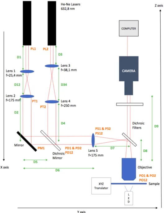
Figure 3.1 : The setup of the optical tweezer. ... 23
Figure 4.1 : Irradiance profile of a Gaussian TEM00 mode [94]. ... 28
Figure 4.2 : Diameter of a Gaussian beam [94]. ... 29
Figure 4.3 : Tangent approximation. ... 30
Figure 4.4 : r and q coordinates of optical system. ... 31
Figure 5.1 : The setup of optical tweezer with dimensions and powers ... 35
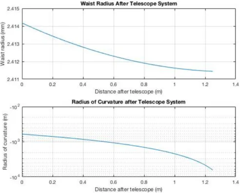
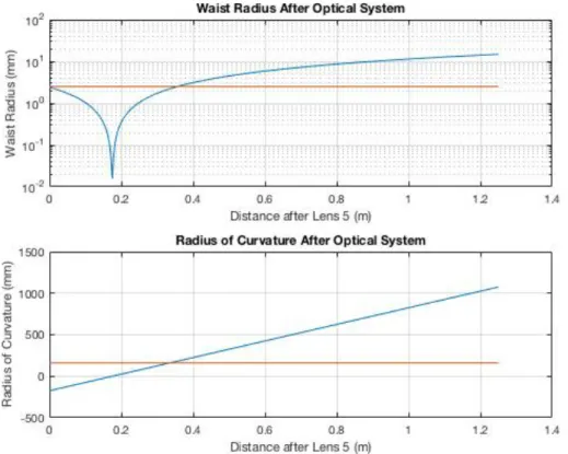
Figure 5.2 : Waist radius and radius of curvature after telescope system for laser 1 37 Figure 5.3 : Waist radius and radius of curvature after telescope system for laser 2 37 Figure 5.4 : Waist radius and radius of curvature after lens 5 for laser 1. ... 38
Figure 5.5 : Waist radius and radius of curvature after lens 5 for laser 2. ... 39
Figure 5.6 : Waist radius after objective for laser 1. ... 39
Figure 5.7 : Waist radius after objective for laser 2. ... 40
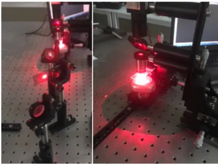
Figure 5.8 : Views of telescopes and lasers in optical tweezer setup ... 41
Figure 5.9 : Views of the mirrors and objective in optical tweezer setup ... 41
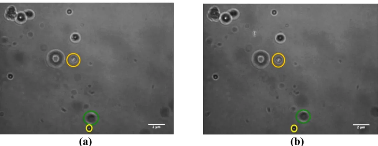
Figure 6.1: Trapped polystyrene bead by laser 1. The trapped polystyrene beads shown in orange circle. The particle which is in green circle was moving while the bead in yellow circle was staying still at a given time. The (a) shows that at the beginning of the trap, and (b) shows that end of the 3 seconds. ... 45
Figure 6.2: Trapped polystyrene bead by laser 2. The trapped polystyrene beads shown in orange circle. It is shown that the particles which are in yellow circle was moving due to the fluid flow. The (a) shows that at the beginning of the trap, and (b) shows that end of the 1,8 seconds. ... 45
Figure 6.3: Trapped polystyrene bead by both lasers simultaneously. The trapped polystyrene beads shown in orange circle by both lasers simultaneously. It is shown that the particle which is in green circle was rotated at a given time. The (a) shows that at the beginning of the trap, and (b) shows that end of the 1,25 seconds. ... 46
Figure 6.4: Moving polystyrene particles. the trapped polystyrene beads by laser 2 shown in red circle. The (a) shows that at the beginning of the trap, at (e) two lasers trapped the bead simultaneously and at (f) only laser 1 trapped the bead at 2 seconds. ... 47
xx
Figure 6.5: Trapping multiple particles. The polystyrene particle trapped by laser 2 and move to laser 1 in Figure 6.5 (a-c). At (d), laser 2 leaving the bead to laser 1 and at (e) laser 2 saperated from trapping region. ... 48 Figure 6.6: Stiffnesses of lasers ... 49 Figure 6.7: Trapping forces on the polystyrene beads ... 49 Figure 6.8: Trapping of yeast cells (Laser 1).The cell in yellow circle was moving
while the yeast cell in red circle was trapping. (a) shows the beginning of the trap moment and (b) is the end of 3 seconds. ... 51 Figure 6.9: Comparison of trapping forces on the polystyrene beads and yeast cells
(Laser 1) ... 51 Figure 6.10: Comparison of stiffnesses for the polystyrene beads and yeast cells
(Laser 1) ... 51 Figure 6.11: Trapping yeast cells (Laser 2). Trapped yeast cell by laser 2 is shown in
orange circle and trapped yeast cell by laser 1 is shown in yellow circle. The cell in blue circle was moving while others trapping. (a) indicates the beginning of the trap and (b) indicates the end of the 1.9 seconds. ... 52 Figure 6.12: Comparison of stiffness for the polystyrene beads and yeast cells
(Laser 2) ... 53 Figure 6.13: Comparison of trapping forces on the polystyrene beads and yeast cells
(Laser 2) ... 53 Figure 6.14: Trapping multiple yeast cells. (a) and (b) show that movement of
trapped yeast cell in green circle by laser 2. (c) shows that trapping multiple cells which are in yellow circle by both lasers simultaneously. ... 54 Figure 6.15: Trapping multiple yeast cells. Trapped yeast cells is shown in red circle (a-b) and in (c) yeast cells trapped by both lasers simultaneously. ... 54 Figure 6.16: Trapping force for cytoplasmic medium (Laser 1) ... 56 Figure 6.17: Stiffness for cytoplasmic medium (Laser 1) ... 56 Figure 6.18: Trapping force for cytoplasmic medium (Laser 2) ... 57 Figure 6.19: Stiffness for cytoplasmic medium (Laser 2) ... 57 Figure 6.20: Trapping Efficiencies ... 58
xxi
CUSTOM DESIGNED OPTICAL TWEEZER FOR TRAPPING YEAST CELLS
ABSTRACT
The goal of this study is developing custom designed optical tweezer which uses two He-Ne lasers (λ=632.8 nm) parallel to each other to trap yeast cells. The characteristic specs of this optical tweezer determined by Brownian Motion of polystyrene beads in water. Stiffness and trapping forces of optical tweezer calculated for laser 1, laser 2 and when both lasers used simultaneously. Laser 2 can trap and move particle to laser 1 and multiple particles can be trapped by the laser 1. After determination of specs of optical tweezer, yeast cells in yogurt culture medium were trapped by laser 1 and laser 2. Stiffness of optical tweezer and trapping force on yeast cells were determined by drag force and Brownian motion methods by assuming the medium was homogenous and had viscosity of 0.038 kg/ms. Viscosity depends on the concentration of fluid and surface. Viscosity of the yogurt culture medium which was used in experiments was calculated theoretically with respect to velocity of fluid and specs of optical tweezer calculated previously. Possibility of application inside yeast cells was studied theoretically by using viscosity of cytoplasmic medium. As a result of this study, this custom designed optical tweezer which uses two He-Ne lasers are applicable in life sciences like inside cells, viscosity measurements and drug delivery systems.
xxiii
ÖZEL YAPIM OPTİK CIMBIZ İLE MAYA HÜCRESİ MANİPÜLASYONU ÖZET
Bu çalışmanın amacı maya hücrelerini yakalamak için iki adet birbirine paralel He-Ne lazer (λ=632.8 nm) kullanan özel yapım optik cımbız geliştirmektir. Bu optik cımbızın karakteristik özellikleri su içerisindeki polisitiren küreciklerinin Brownian hareketleriyle belirlenmiştir. Optik cımbızın sertliği ve yakalama kuvvetleri lazer 1, lazer 2 ve her iki lazerin aynı anda kullanıldığı zaman için hesaplanmıştır. Lazer 2 parçacıkları yakalayıp lazer 1’e taşıyabilmektedir ve birden fazla parçacık lazer 2 tarafından yakalanabilmektedir. Optik cımbızın özellikleri tanımlandıktan sonra yoğurt kültürü içindeki maya hücreleri lazer 1 ve lazer 2 tarafından yakalanmıştır. Optik cımbızın sertliği ve maya hücreleri üzerindeki yakalama kuvveti ortamın homojen ve viskozitesinin 0.038 kg/ms olduğunu kabul ederek Brownian hareketi ve sürüklenme kuvveti methodlarıyla belirlenmiştir. Viskozite konsantrasyona ve yüzeye bağlı olarak değişmektedir. Deneylerde kullanılan yoğurt kültürünün viskozitesi akışkanın hızına ve optik cımbızın özelliklerine göre teorik olarak hesaplanmıştır. Hücre içinde uygulanma ihtimali için hücre sitoplazmasının viskozitesi kullanılarak teorik olarak çalışılmıştır. Bu çalışmanın sonucu olarak; bu 2 adet He-Ne lazer kullanan özel yapım optik cımbız; hücre içinde, viskozite ölçümleri ve ilaç taşınımı gibi fen bilimleri uygulamalarında kullanılabilmektedir.
1 1. INTRODUCTION
Optical tweezers are defined as the highly focused laser beams which can trap and manipulate the particles between nanometer and micrometer size range by means of radiation pressure. In 1970, Ashkin was reported that particles were accelerated by radiation pressure [1]. In 1986, For optical trapping of dielectric particles, single highly focused laser beam was developed by focusing laser beam into high numerical aperture objective [2]. They have been used in biological applications such as molecular motors studies, single molecule experiments and cellular manipulation since 1987 when Ashkin and Dziedzic trap bacteria and viruses by using green laser [3,4]. Instead of just a manipulation of particles, optical tweezers can be used to control or measure the forces on biological processes[5].
The trapping mechanism is the result of the exchange of momentum between trapping light and trapped particle. Resulting force occurs due to momentum exchange and depends on the size of particle: Ray optics approximation, Rayleigh approximation and Generalized Lorenz-Mie Theory.
The gradient force and the scattering force form the net force on the particle. Scattering force pushes the particle in the direction of beam propagation whereas gradient force pulls the particle towards the higher internsity regions. Stable trapping can be achieved when the gradient force is greater than the scattering force [5,6]. Assuming that trapping potential is harmonic and trapping force can be characterized by several calibration methods. Force can be calculated by the measuring the displacement of the beam from the trap center and fluid velocity. This force is the drag force and it is assumed that drag force equals to trapping force. Another way of measuring the trap force is Brownian Motion Method. In Brownian Motion Method, trap stiffness can be determined without any information about viscosity of fluid and geometry of particle [7,8].
2
1.1 Historical Background of Optical Tweezers
Optical tweezers demonstrate that light is able to exert a force on matter. Quantum theory states the momentum carried per photon. Prior to quantum mechanics, it is predicted that there exist “radiation pressure” as a result of electromagnetic theory developed by James Clerk Maxwell [9]. It describes that there is a pressure in the direction normal to the wave in a medium where the waves are propagated and it numerically equals to the energy contained in unit volume [10].
Bartoli predicted such pressure in thermodynamic context which is called as Maxwell-Bartoli force [11] and Crooks discovered the radiometric forces [12]. Two papers published by P.N. Lebedew and by E. F. Nichols and G. F. Hull in 1901. Papers had independent results but same approximation to study the effect of the light, produced by an arc lamp, had on thin vanes. Low gas pressures and thin metallic vanes were used by Lebedew on the contrary high pressure gas and silvered glass vanes used by Nichols and Hull [13,14]. In second paper, measurements were carried out for providing the validation of results of Nichols and Hulls in the high pressure limit since the gas could be neglected over short exposures of the vanes to the light [15]. Nichols and Hulls analysed the experiments in accordance with their historical backgrounds and compared them. As a conclusion, they found that both experiments had measurement errors but both qualitatively proved the existence of the radiation pressure without quantitatively following the theory of Maxwell-Bartoli forces. In 1903, Nichols and Hull published the quantitative demonstration [15]. Studies of optical manipulation began by Arthur Ashkin in 1970s. Although discovery of lasers has provided convenience to study optical forces due to much higher intensities of lasers, optical forces are dominated by radiometric forces and it is too difficult to observe their direct effects. Ashkin could observe the radiation pressure due to reflection from such particles by using transparent particle and transparent medium while avoiding heating problems. In 1970, he found that particles were trapped by the laser beam and travelled in the direction of beam propagation [1]. He has demonstrated that gradient force is created by intensity gradient of the laser beam, pulls the high-refractive-index particles toward the beam axis and push low-refractive-index particles away from the axis. He hypothesized
3
that light could rotate and accelerate the particles. He also discussed about magneto-optical trap and atomic dipole trap. By using two beams which propagates against each other, an optical trap can be created where particles are under influence of a combination of gradient force and radiation pressure [10].
The next year, Ashkin and J. M. Dziedzic as a co-author trapped glass beads suspended in air by single laser beam which was directed upward so that the radiation pressure balances the gravitational force on the particle. They observed that if the beam was turned off after dragging, the bead was allowed to go back to equilibrium position without oscillation. Moreover, they said that laser modes different from the normal TEM00 Gaussian beam, such as TEM01 and TEM01*, a
doughnut mode could be used [16]. Ashkin also found that this new technique was possible in high vacuum and for stabilizing particle position by using feedback mechanism [10,17,18]. He observed new types of nonlinear effects and studied the effect of radiation pressure on a liquid interface [19,20].
In 1970s, optical levitation of droplets was studied most as application of optical manipulation. Ashkin and Dziedzic studied how both solid and liquid airborne particles can be trapped and the ways of carrying types of experiments such as crystallization and simple measurements on particle interactions. This paper also shows problems due to optical levitation, such as trapping multiple particles but not controlling them independently [21].
Ashkin and Dziedzic show how to make sensitive measurements on levitated droplets by stabilization method [22]. In this paper, they studied effects of wavelength and size on variations of optical forces. Size determination was provided highly sensitive by the resonances excited within the droplets. This technique is commonly used for size measurement now, and it can be combined with other techniques such as Raman spectroscopy [23], to determine the size and composition of particle.
In 1986, Ashkin, Dziedzic, Bjorkholm, and Chu studied trapping with single beam laser focusing through high numerical aperture (NA) microscope objective. By this way, the particle could be trapped in the plane transverse to the laser beam propagation and in the axial direction. Therefore, the particles could be trapped by
4
beam directed downward and they were held against gravity. They demonstrated a tweezer which has second beam to guide particles into trapping region. Tweezer was able to trap particles between 25 nm and 10 µm [2].
They open new size regime to optical trapping by optical tweezers. Ashkin and Dziedzic were the first ones who trap bacteria and viruses by optical tweezers which used green laser [3]. Green laser has disadvantages on trapping biological samples since biological samples absorbs strongly green laser therefore they are easily damaged. In 1987, Ashkin and his collegues overcomed this problem by using infrared laser to trap cells without damaging. The usage of infrared beams is important for biological experiments, in almost all biological experiments such wavelengths are used.
1.2 Applications of Optical Tweezers
New viewpoints in microscopic world to manipulation of small objects have been created by trapping and movement of particles. Optical tweezers have been used for cell sorting, actively alteration of polymer structures, application of stall forces, characterization of molecular motors and measurement of binding forces in the biological and medical fields.
For cellular manipulation and cell sorting techniques, optical tweezers have many advantages than other mechanical techniques. It is possible that in vitro manipulation of cells with light is sterile and without harming the cells. Trapping of up to 10 Escherichia coli (E. Coli) bacteria cells of 2 µm in length was trapped and manipulated by using 1064-nm laser tweezer quasi-simultaneously [24]. And control of the molecules in the cell without damaging cell wall is possible [25,26]. Altering the choromosome movement on to mitotic spindle in vitro [27], accelerating cell-cell interaction by bringing active retinal cells together [28], manipulation of vesicles for membrane fusion [29] can be examples of the studies for micromanipulation applications of optical tweezers.
Optical tweezers can be used to manipulate organelles. The trapping force on lipid granules inside yeast cell was measured between 10 and 60 pN due to change of viscosity of the yeast cells in 0.1-0.8 Pas range by 830-nm laser tweezer [30]. In
5
addition to inside cells, optical tweezers can be used in rheology and quantitative measurements of biological acitivites for in vivo applications. Flowing RBCs in blood capillaries of living animal was trapped and manipulated by infrared laser tweezers. The capillaries was blocked with RBCs and then was cleared with optical tweezers [31]. Also, cells and nanoparticles inside living zebrafish were trapped with 1064-nm laser [32].
In rheology applications, optical tweezers can be used for measurement the microscopic viscosity as a confocal probe [33] or they combined with optical microscopy in order to map the fluid flow and measure the viscosity [34,35]
Optical trapping in different surfaces has been developed in order to maximize efficiency of optical tweezers. Optical trapping of mammalian, yeast and Escherichia coli cells on the surface of two-dimensional photonic crystal was developed in order to minimize cell-damaging and increase cell viability in cell manipulation techniques [36]. The effect of trap position to focal waist in the vicinity of the reflecting surface in optical tweezer was studied [37]. As a surface, random gold nano-island substrates used for trapping of assembling of particles and live cells. Near-field optical trapping force and long-range thermophoretic force, which overcomes the axial convective drag force, creates trapping effect. Lateral convection pushes the samples into trapping region [38].
Two of the main applications of optical tweezers are study of molecular motors and physical properties of DNA. In both applications, biological sample is biochemically attached to polystyrene beads or glass beads in micron-sized range. By this way, the force and step size of the molecular motor can be measured. Block et al. improved the efficiency of kinesin motors as well as Svoboda et al. measured step size of kinesin on microtubules as 8 nm by combining with interferometry [39,40]. Moreover, elasticity of double and single stranded DNA molecules was determined by using optical tweezers [41]. Rigidity and bond breaking force was determined by applying torque to actin filaments [42]. In order to understand a cell division process of eukayotic organisms, minimum trapping force to move isolated single mammalian chromosome was determined to be »0.8-5 pN by using 1064 nm laser tweezer [43].
6
Mechanical properties of double-stranded DNA were determined by using 1064-nm laser tweezers [44].
Observing phase transitions in colloidal suspensions [45] and measuring entropic extraction in giant vesicles [46] can be set examples as applications of optical tweezers in colloidal systems.
For applications in statistical physics, escape of a Brownian particle from a coupled-tweezer trap was synchronized by using stochastic resonance [47]. Wang et al. experimentally demonstrated that the second law of thermodynamics has not been favorable for small systems and short timescales by using optical tweezers [48]. Besides polystene beads; absorbing particles [49], metallic particles [50,51,52], quantum dots [53], carbon nanotubes [54] and fluorescent beads[55] have also been trapped as well.
7
2. THE BASICS OF THE OPTICAL TWEEZER 2.1 Physical Principle of Optical Tweezer
Optical tweezers use the forces of laser radiation pressure to trap and manipulate microscopic particles. The trapping force (FT) is a combination of two forces: a
gradient force (FG) and the scattering force (FS) and determined by relation:
𝐹: = 𝐹<+ 𝐹> (2.1)
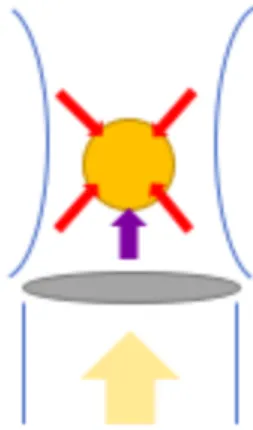
The photon of the incident laser beam applies the pressure against the surface of the trapped particle and as result the gradient force arises whereas the scattering force arises from the change in velocity due to movement of light between mediums of two different indices of refraction. By the reason of the dependence of momentum on velocity and conservation of momentum, the trapped particle moves with equal but opposite momentum of the photons i.e. in the direction of incident light (Figure 2.1). [6].
Figure 2.1: Optical forces. Gradient force is shown in red; scattering force is shown in purple.
If the size of the particles is larger than the wavelength of the trapping laser, principle of optical trapping is explained with ray optics; whereas particle is much smaller it is explained with dipole or Rayleigh approximation. In most experiments, the sizes of particles are comparable with the wavelength of the trapping laser. In this
8
case, instead of ray optics and Rayleigh approximation, electromagnetic theory of light is used. In order to calculate trapping forces in this range, generalized Lorenz-Mie theory is used [56,57].
2.1.1 Ray Optics approximation
The simple ray optics model of the single-beam gradient trap calculates the trapping forces on sphere of diameter larger than wavelength of light (R > 10 λ) [57,58]. In the ray optics or geometrical optics regime, total light beam is seperated into individual rays. Each ray has appropriate intensity, direction, polarization and the characteristics of a plane wave of zero wavelength. By this specs they can change directions by reflection and refraction and changes polarization according to the usual Fresnel formulas. This regime neglects diffractive effects [58].
Due to the neglect of surface reflection from the particle, the particle is trapped at the focus of the laser beam (Figure 2.2a). Therefore, there is no net force on the particle when the particle trapped at the focus. The particle leaving the traping the restoring force is formed to pull particle back to trap center (Figure 2.2b-c).
(a) (b) (c)
Figure 2.2: Qualitative view of optical trapping of dielectric spheres [57]. Whereas the surface reflection from the particle was neglected in above discussion; in reality, it has to be considered. Particle is pushed forward by the photons reflected back by the surface. In case of this force is greater than restoring force, particle is pushed forward and can not be trapped. The surface reflection depends on the relative refractive indices of the particle and the medium.
𝑚 = 𝒏𝒑
𝒏𝒎𝒅 (2.2)
𝑛A and 𝑛BC are the refractive indexes of particle and medium, respectively. Larger
m indicates more surface reflection and therefore greater difficulty in trapping the microsphere with an optical tweezer. In order to increase the restoring force, the laser
9
beam should be highly focused by a high numerical aperture (NA) objective lenses. For the Ray optics approximation for single ray with power P, the gradient and scattering forces are determined as below (Figure 2.3).
Figure 2.3: Ray propagation into dielectric sphere for ray optics approximation [25]. The ray is exposed both reflection, R and transmission T at all surfaces. 𝑛 signifies the normal to the surface of the sphere.
𝐹> = 7DEF G 1 + 𝑅 cos 2𝜃 − 𝑇 Q RST QUVQW XY RST QU ZXY[XQY RST QW (2.3) 𝐹< = 7DEF G 𝑅 sin 2𝜃 − 𝑇 Q T^_ QUVQW XY T^_ QU ZXY[XQY T^_ QW (2.4)
P is the power of the ray, 𝜃 and 𝜑 are the angles of the incident and refracted rays, respectively. 7DEF
G is the momentum per second transferred by the ray. R is Fresnel reflection coefficient and T is the fresnel transmission coefficient. These coefficients give the fraction of the light being reflected or transmitted at an interaction [25]. 2.1.2 Rayleigh approximation
If the size of particle is smaller than the wavelength of the light (R < λ/10), the optical tweezer forces can be calculated by Rayleigh approximation [59]. The gradient in the electromagnetic field causes a force induced on the particle proportional to the gradient of the field and therefore proportional to the gradient of the intensity of the light. Intensity maximum is in the centre of the highly focused Gaussian beam for giving rise to a three-dimensional gradient of the laser light, which produces a force directed to the centre. The gradient force, Fg, is induced by
10 the field and described as,
𝐹< =Qabc7DE
G
B[VZ
B[XQ ∇𝐼 (2.5)
𝑐 is the speed of the light, 𝑎 is the radius of the object, 𝑚 the effective index of reflection as described in equation (2.2) and 𝐼 is the intensity of the light. It is shown that the gradient force is proportional to the volume of the particle and to the gradient of the intensity of the trapping light, i.e., 𝐹< ∝ ∇𝐼 [25,57].
The scattering force, Fs, is proportional to the intensity of the light and described as, 𝐹> = ZQiajbk7DE
lmnG
B[VZ
B[XQ 𝐼 (2.6)
The particle is attracted into the region of the highest intensity by gradient force, whereas the scattering force pulls the particle into an equilibrium position which is not at maximum intensity. Stable trapping is occured by competition of these forces [58,60]. Also, the size of the particle affects the gradient and scattering forces. For large particles, the scattering force is dominating and that it is resulted to trapping unstable [25].
2.1.3 Generalized Lorenz-Mie theory
When the sizes of particle are comparable with the wavelength of the trapping laser, electromagnetic theory of light has to be used [57,60]. Generalized Lorenz-Mie theory (GLMT) includes the equations of light scattering of a beam. Beam fields incident on the particle must be known for calculation of scattering by a transversely localized beam. The exact fields of beam complying with both the wave equation and Maxwell’s equations are not in closed form, excepting plane wave. In order to explain this dificulty, transversely localized beam is expressed in 3 approaches: an angular spectrum of plane waves, the fields in terms of infinite series of spherical multipole partial waves with specified coefficients, analytic approximations of the beam field. GLMT calculations generally use second and third approaches [61]. For the fundamental TEM00 mode of laser beam, the electric and magnetic fields of a
monochromatic Gaussiam beam is described as: 𝑬 𝑥, 𝑦, 𝑧 = 𝐸sexp −xw[
11 𝑩 𝑥, 𝑦, 𝑧 = (𝐸s/𝑐) exp −w
[
xy[ exp 𝑖𝑘𝑧 𝒖𝒚 (2.8)
where c is the speed of the light, 𝐸s is the peak electric field strength, w0 is the
electric field half-width. The Gaussian beam of wavelength l and wave number k=2p/l is linearly polarized in the x direction and propagating in the +z direction. exp(iwt) is time dependence and it is implicit [61].
𝜌Q = 𝑥Q + 𝑦Q (2.9) If the center of the beam is at origin of coordinates, beam is on-axis related and thus it lies on the beam’s symmetry axis.
Equations (2.7) and (2.8) ignore the diffraction of the beam. If the Gaussian beam fields are Fresnel diffracted from z=0 to z>0, electric and magnetic fields are defined as: 𝑬 𝑥, 𝑦, 𝑧 = 𝐷𝐸sexp −„wx[ y [ exp 𝑖𝑘𝑧 𝒖𝒙 (2.10) 𝑩 𝑥, 𝑦, 𝑧 = (𝐷𝐸s/𝑐) exp −„w [ xy[ exp 𝑖𝑘𝑧 𝒖𝒚 (2.11)
where the D is given as:
𝐷 = 1 +Q…>†x
y
VZ
(2.12) where the s is beam confinement parameter and defined as:
𝑠 = 1/𝑘𝑤s (2.13) The beam becomes freely propagating focused Gaussian beam since it spreads tranversely with its minimum width w0 in the z=0 plane. Beam confinement
parameter has to be equal or less than 1/p because a beam must be tranversely confined at least of its wavelength. If the 𝑠 ≪ 1/𝜋, a beam is loosely focused since its tranverse spreading goes on narrow and becomes only slowly as a function of z. If the 𝑠 ≈ 1/𝜋, a beam is tightly focused since its tranverse spreading is wide and develops as a function of z. Equations (2.10) and (2.11) has the limits 𝑤s → ∞ or 𝑠 → 0 which means that is a plane wave [61].
12
for full wave equation or Maxwell’s equations. In order to obtain a beam in the form of infinite series in powers of s the procedure has been developed which is both exact solution of wave equation and Maxwell’s equations. The procedure has the Gaussian beam of equations (2.10) and (2.11) as its zeroth order term [62,63]. s5 order of the
expansion of the beam fields is given as, 𝑬 𝑥, 𝑦, 𝑧 = 𝐷𝐸sexp −„wx[ y[ exp 𝑖𝑘𝑧 [𝑒•𝒖𝒙+ 𝑒•𝒖𝒚− 2𝑖𝐷 • xy 𝑒†𝒖𝒛] (2.14) 𝑩 𝑥, 𝑦, 𝑧 = (𝐷𝐸s/𝑐) exp −„w[ xy[ exp 𝑖𝑘𝑧 [𝑏•𝒖𝒙+ 𝑏•𝒖𝒚− 2𝑖𝐷 • xy 𝑏†𝒖𝒛] (2.15) where 𝑒• = 1 + 𝑠Q 𝐷 𝑤s Q 2𝑥Q+ 𝜌Q− 𝐷 𝜌” 𝑤sQ +𝑠” „ xy ” 𝜌Q 2𝜌Q+ 8𝑥Q− 3𝐷 wn xy[ − 2𝐷 •[w[ xy[ + 𝐷 Q wk Qxyn (2.16) 𝑏•= 1 + 𝑠Q 𝐷 𝑤s Q 2𝑦Q+ 𝜌Q− 𝐷 𝜌” 𝑤sQ +𝑠” „ xy ” 𝜌Q 2𝜌Q+ 8𝑦Q− 3𝐷 wn xy[ − 2𝐷 •[w[ xy[ + 𝐷Q wk Qxyn (2.17) 𝑒•= 𝑏• = 𝑠Q x„ y Q 2𝑥𝑦 + 𝑠” „ xy ” 2𝑥𝑦 4𝜌Q− 𝐷 wn xy[ (2.18) 𝑒† = 𝑏† = 𝑠 + 𝑠l 𝐷 𝑤s Q 3𝜌Q− 𝐷 𝜌” 𝑤sQ + 𝑠˜ „ xy ” 𝜌Q 10𝜌Q− 5𝐷 wn xy[ + 𝐷Q wk Qxyn (2.19)
In the above equations, s is determined as L approximation of the exact TEM00 laser
beam. s converges rapidly near the focal waist and slowly only when 𝜌Q is greater than 𝑤sQ+ 4𝑠Q𝑧Q. When the focal waist of the beam moved from the origin to other point which is favorable translation of coordinates, the translated beam is called off-axis related to scatterer whose center is not along the beam’s symmetry off-axis [61]. It is assumed that exact electric and magnetic fields of the incident beam, which is considered as arbitrary tranversely localized, on a homogeneous sphere of radius a and refractive index 𝑛A and centered at origin of coordinates, the TE and TM
13
Bromwich potentials of the beam in spherical coordinates are given by [61,64,65]
𝑈:•žŸbB 𝑟, 𝜃, 𝜑 = •y ¡ 𝑖7𝑐7 Ax𝑔 7,:•B 𝜓7(𝑘𝑟) 7 B¤V7 ∞ 7¤Z 𝑃7B cos 𝜃 exp (𝑖𝑚𝜑) (2.20) 𝑈:¦žŸbB 𝑟, 𝜃, 𝜑 = •y ¡ 𝑖7𝑐7 Ax𝑔 7,:¦B 𝜓7(𝑘𝑟) 7 B¤V7 ∞ 7¤Z 𝑃7B cos 𝜃 exp (𝑖𝑚𝜑) (2.21) where 𝑐7Ax = (2𝑛 + 1)/[2𝑛 𝑛 + 1 ] (2.22) 𝐸s is the maximum strength of the electric field of the beam. 𝜓7and 𝑃7Bare the Ricatti-Bessel and Legendre functions, respectively. 𝑔7,:•B and 𝑔
7,:¦B are the beam shape coefficients. Electric and magnetic field are obtained by vector derivatives of equations (2.20) and (2.21). Beam shape coefficients is important for GLMT since the scattered intensity and all quantities derived from it are calculated by combination of beam shape coefficients, angular functions and an plane wave
function of LMT and bn partial wave function of LMT.
According to equations (2.20) and (2.21) and beam shape coefficients are given
𝑔7,:•B = −𝑖 7VZ 2𝜋 𝑘𝑟 𝑗7 𝑘𝑟 𝑛 − 𝑚 ! 𝑛 + 𝑚 ! sin 𝜃 𝑑𝜃 a s 𝑑𝜑 Qa s ×𝑃7B cos 𝜃 exp −𝑖𝑚𝜑 𝑐𝐵¬bCžŸbB 𝑟, 𝜃, 𝜑 (2.23) 𝑔7,:¦B = −𝑖 7VZ 2𝜋 𝑘𝑟 𝑗7 𝑘𝑟 𝑛 − 𝑚 ! 𝑛 + 𝑚 ! sin 𝜃 𝑑𝜃 a s 𝑑𝜑 Qa s ×𝑃7B cos 𝜃 exp −𝑖𝑚𝜑 𝐸¬bCžŸbB 𝑟, 𝜃, 𝜑 (2.24) where 𝐸¬bCžŸbB and 𝐵
¬bCžŸbB are the radial components of the presumably known beam fields in spherical coordinates. If the beam is on-axis in compliance with sphere, only m=±1 beam shape coefficients are not zero due to the structure of the 𝜑 integral and they are defined as:
𝑔7,:•Z = −𝑖𝑔
7,:• (2.25) 𝑔7,:•VZ = 𝑖𝑔
7,:• (2.26) 𝑔7,:¦±Z = 𝑔7,:¦ (2.27) If Gaussian beam propagates freely, 𝑔7,:• equals to 𝑔7,:¦. But more general beams
14
(laser beam) transmitted high numerical aperture lens 𝑔7,:• is different from 𝑔7,:¦. Since assuming that the Maxwell’s equations are solved by the beam, the radial dependence of angular integrals stops the kr/jn(kr) which is prefactor. The resulting
beam shape coefficients become constants. But if the beam shape coefficients are not solutions of Maxwell’s equations, the beam shape coefficients are obtained from equations (2.23) and (2.24) without cancellations. In order to obtain constant coefficients, the value r is identified at a convenient location or right-hand side are integrated with respect to r from the origin to infinity. Both of these ways define a new beam by the beam shape coefficients by equations (2.20) and (2.21) in order to renormalize the original beam and repair the defect of not being exact solution of Maxwell’s equation. The original beam is strongly resembled by the new beam in the region where the scattered fields are largest due to large field strength [61].
According to equations (2.20) and (2.21), for the scattering of beam by a sphere, scattered and interior Bromwich potentials are given,
𝑈:•>Gb®® 𝑟, 𝜃, 𝜑 = − •y ¡ 𝑖 7𝑐 7Ax𝐵7B𝜁7Z 𝑘𝑟 7 B¤V7 ∞ 7¤Z 𝑃7B cos 𝜃 exp 𝑖𝑚𝜑 (2.28) 𝑈:¦>Gb®® 𝑟, 𝜃, 𝜑 = − •y ¡ 𝑖 7𝑐 7Ax𝐴7B𝜁7(Z)(𝑘𝑟) 7 B¤V7 ∞ 7¤Z 𝑃7B cos 𝜃 exp (𝑖𝑚𝜑) (2.29) and 𝑈:•…7®Ÿ¬…°¬ 𝑟, 𝜃, 𝜑 = ∞7¤Z 7B¤V7 ±•¡y 𝑖7𝑐7Ax𝐷7B𝜓7(𝑁𝑘𝑟)𝑃7B cos 𝜃 exp (𝑖𝑚𝜑) (2.30) 𝑈:¦…7®Ÿ¬…°¬ 𝑟, 𝜃, 𝜑 = ∞7¤Z 7B¤V7 ±•¡y 𝑖7𝑐7Ax𝐶7B𝜓7(𝑁𝑘𝑟)𝑃7B cos 𝜃 exp (𝑖𝑚𝜑) (2.31)
where 𝜁7(Z) are Ricatti-Henkel functions, 𝐴7Band 𝐵
7B are defined as partial wave scattering amplitudes and 𝐶7Band 𝐷7B are described as the partial wave interior amplitudes. These are obtained by matching the boundary conditions for various components of electric and magnetic fields at the sphere:
𝐴7B= 𝑎 7𝑔7,:¦B (2.32) 𝐵7B = 𝑏 7𝑔7,:•B (2.33) 𝐶7B = 𝑐 7𝑔7,:¦B (2.34) 𝐷7B= 𝑑 7𝑔7,:•B (2.35)
15
The scattered fields are various vector derivatives of the Bromwich potentials of equations (2.30) and (2.31). For the r goes to infinity, scattered intensity defined as
𝐼>Gb®® 𝑟, 𝜃, 𝜑 = 𝐸sQ/𝜇
s𝑐 1/𝑘𝑟 Q 𝑆Z(𝜃, 𝜑) Q+ 𝑆Q(𝜃, 𝜑)Q (2.36)
where 𝜇s is permeability of free space and the 𝑆Z(𝜃, 𝜑) and 𝑆Q(𝜃, 𝜑) are the total scattering amplitudes. 𝑆Z 𝜃, 𝜑 = − 7 𝑐7Ax[−𝑖𝑚 B¤V7 ∞ 7¤Z 𝑎7𝑔7,:¦B 𝜋7B 𝜃 + 𝑏7𝑔7,:•B 𝜏7B 𝜃 ]exp (𝑖𝑚𝜑) (2.37) 𝑆Q 𝜃, 𝜑 = − 7 𝑐7Ax[−𝑖𝑚 B¤V7 ∞ 7¤Z 𝑏7𝑔7,:•B 𝜋7B 𝜃 + 𝑎7𝑔7,:¦B 𝜏7B 𝜃 ]exp (𝑖𝑚𝜑) (2.38)
and the angular functions are defined as below.
𝜋7B 𝜃 = T^_ UZ 𝑃7B cos 𝜃 (2.39)
𝜏7B 𝜃 = 𝑑/𝑑𝜃 𝑃7B cos 𝜃 (2.40) GLMT formulas have also been derivations of the scattered power and scattered cross section [64], the radiation force on the sphere [64,66,67] and the radiation torque [66,68].
This method becomes complex when hundreds and thousands are required for scattering of beam from large particle with 2pa/l≫1. If the s≪1, localized model of the coefficients which is based upon van de Hulst’s association in LMT of the incident ray impact parameter kr with partial wave number n+1/2 is an alternative to this method. Given the fact that the center of a Gaussian beam’s focal waist is located at (𝑥s = 𝜌scos 𝜑s , 𝑦s = 𝜌ssin 𝜑s , 𝑧s), the localized model coefficients are defined below [69,70].
𝑔7,:•B = (−𝑖𝐹 7) −𝑖𝑒𝑥𝑝 −𝑖𝜑s / 𝑛 + 1/2 BVZ 𝐼BVZ 𝑄 − exp (−2𝑖𝜑s)𝐼BXZ 𝑄 (2.41) 𝑔7,:•s = 𝐹 7 Q…7 7XZ7XZ Q sin 𝜑0 𝐼1(𝑄) (2.42) 𝑔7,:•VB = (−𝑖𝐹 7) −𝑖𝑒𝑥𝑝 𝑖𝜑s / 𝑛 + 1/2 BVZ 𝐼BVZ 𝑄 − exp (2𝑖𝜑s)𝐼BXZ 𝑄 (2.43) 𝑔7,:¦B = 𝐹 7 −𝑖𝑒𝑥𝑝 −𝑖𝜑s / 𝑛 + 1/2 BVZ 𝐼BVZ 𝑄 − exp (−2𝑖𝜑s)𝐼BXZ 𝑄 (2.44) 𝑔7,:¦s = 𝐹 7 Q…7 7XZ7XZ Q cos 𝜑0 𝐼1(𝑄) (2.45) 𝑔7,:¦VB = 𝐹7 −𝑖𝑒𝑥𝑝 𝑖𝜑s / 𝑛 + 1/2 BVZ 𝐼BVZ 𝑄 − exp (2𝑖𝜑s)𝐼BXZ 𝑄 (2.46)
16 where 𝐹7 = 𝐷sexp −„ywy [ xy[ 𝑒𝑥𝑝 −𝐷s𝑠 Q 𝑛 + 1 2 Q exp (−𝑖𝑘𝑧 s) (2.47) 𝐷s = 1 − 2𝑖𝑠 †y xy VZ (2.48) 𝑄 = 2𝐷s𝑠 𝑛 + 1 2 (𝜌s 𝑤s) (2.49) and Im are modified Bessel functions.
When the beam is on-axis, these focused Gaussian beam coefficients as simplified as 𝑔7,:• = 𝑔7,:¦ = 𝐷s𝑒𝑥𝑝 −𝐷s𝑠Q 𝑛 + 1 2 2 exp (−𝑖𝑘𝑧s) (2.50) In the plane wave, 𝑔7,:• = 𝑔7,:¦ = 1 limits the LMT. The localized beam shape coefficients in equations (2.20) and (2.21) define a beam which is exact solution of Maxwell’s equations. It has been studied the reason why localized beam shape coefficients are related to Fresnel diffracted fields rather than Davis-Barton fields [71,72,73,74,75]. The localized model coefficients are derivation of general principles, and the beam defined by the localized coefficients performs to expect the behavior of the higher order Davis-Barton beams.
For other beam types, localized models have been derived from GLMT scattering calculations for scattering of a beam with s≪1 and large particle with 2pa/l≫1 [75,76,77,78,79,80]. Localized models have been developed for scattering by a circular [81] or elliptical cylinder [82]. Also, the procedure used experimently in order to measure beam shape coefficients [83,84].
By the means of beam shape coefficients, optical force can be calculated by using cross sections in x, y and z axis for radiation force [59,64].
𝑭 𝒓 =7DE
G 𝐼s 𝒙𝐶A¬,• 𝒓 + 𝒚𝐶A¬,• 𝒓 + 𝒛𝐶A¬,†(𝒓) (2.51) where P is the power of the laser and I0 equals to intensity of beam at center of the
17 2.2 Trapping Efficiency
For optimizing the optical trapping, trapping efficiency must be considered as well as magnitude of the trapping force on the dielectric particle. The force is related to trapping beam power.
𝐹 =½7DEF
G (2.52) where F is force on the particle in an optical trap, Q is defined trapping efficiency, P is the beam power of the laser at trapping plane. Higher Q means higher trapping efficiency. 𝑛BC𝑃/𝑐 defines the incident flux from the laser in a medium with refraction index 𝑛BC, c is the speed of the light trapping [87].
Intensity distribution of the light at entrance of the microscope determines the trapping efficiency. In Ray optics approximation, it is predicted that overfilling the microscope objective can make the efficiency higher. Diameter of the incident laser beam is greater then the objective opening, trimming the outer portion of the beam. The farther rays entering the objective with steepest angles, make an increase in intensity related to central on-axis beams. Thus, the axial trapping efficiency increases since gradient force is getting greater than scattering force. For lateral trapping, the effect of overfilling is clear since particle size have come up with conflict results.
2.3 Detection and Calibration of Optical Forces 2.3.1 Force detection techniques
Optical tweezers can measure and apply forces on spheres besides trapping the particles for manipulation. The particle is confined in a three-dimensional harmonic potential by optical trap (Figure 2.4). Single direction of this potential can be defined as E(x)=kx2/2 where k is a harmonic constant. The force is linearly dependent on the displacement. In order to determine the force, position of the bead in a trap should be measured [25].
18
Figure 2.4 :Trapped particle confined in harmonic potential.
In order to measure the position of the trapped particle, quadrant photodiode (QPD) or standard video camera with subsequent particle tracking can be used. QPD measures smaller forces with high time resolutions and nanometer sized displacements at a rate of several kHz. They offer precise, high-bandwidth measurements. However, tracking multiple particles with QPD simultaneously is difficult. Although standard video cameras allow tracking multiple particles with an accuracy of the order of 10 nm and frame rate of about 30 Hz, this frame rate is often slower than typical resonance frequency of an optical trap. High-speed video camera is an alternative to QPD and standard video camera for recording positions of many particles at several kHz. It is showed that both high-speed, full-field , CCD camera and QPD have similar performance for measuring displacement in optical tweezers [88]. CMOS cameras provide reduced field of view frame rates of the order 1kHz, and the data can be managed in real time using a stardard PC [89,90].
2.3.2 Calibration techniques
Various methods for measuring trap forces have been studied. Firstly, there is a drag force method which allows to calculate stiffness and trapping force by using velocity and viscosity of fluid. Second method is equipartition method or Brownian Motion method. In this method, trap force is measured by Boltzmann’s constant, absolute temperature and position data of particle. Escape force methods calculates the force by escape velocity which can be measured by accelerating the particle until it gets out from the optical trap. Fourth method is the power spectrum method which uses the thermal vibrations for calculating stiffness. Last method is step response method which is based on estimation of trapped bead’s response according to movement of the trapped focus [7,8].
19 2.3.2.1 Drag force method
The viscosity and velocity of fluid, size and shape of particles must be known for this method. In this method sample is moved at constant velocity, the occurring force causes displacement of the bead from the laser, x [8]. Stiffness, k, can be calculated as given,
𝑘 = 𝐹®¬bA/𝑥 (2.53) where Ftrap is trapping force. Trapping force equals to the drag force since drag force
can not break the trapping action.
𝐹®¬bA = 𝐹C¬b< = 6𝜋𝜇𝑣À𝑎 (2.54)
where the µ is the dynamic viscosity of the fluid, vf is the velocity of the fluid and 𝑎 is the radius of the particle.
2.3.2.2 Brownian Motion method
Particles suspended in fluid moves randomly due to the collisions with the moving molecules of liquid. This is called as The Brownian Motion. The Brownian motion method uses the thermal fluctuation of the trapped particle, using absolute temperature to measure trap stiffness, k. This stiffness of the tweezer is calculated from the equipartition theorem for a particle fluctuating in a harmonic potential of the trap [7,8]. In equipartition theorem, a molecule in thermal equilibrium has a kinetic energy for each degree of freedom <H>. Assuming that the movement of the trapped particle is resulted from only thermal fluctuations, kinetic energy equals to potential energy of the trap:
𝐻 =ZQ𝑘ž𝑇 = ZQ𝑘 𝑥Q (2.55) where the kb is the Boltzmann’s constant, kb=1.3807x10⁻²³ JK-1 and the T is the absolute temperature. <x2> is the time-averaged square of the bead’s horizontal displacement from the center of the trap. In this method, either particle geometry or viscosity of fluid is not required to calculate the stiffness. The temperature causes random vibration and trap force resists movement from the trap center [7].
20 2.3.2.3 Escape force method
It was the first method to estimate optical trapping [2]. In this method, the force required on the particle to escape from the trap. If the particle slowly is accelerated until it breaks from its trap, the escape force can be measured (Figure 2.5). The trap force simply equals to the escape force caused by the acceleration [8].
𝐹®¬bA = 𝐹Ÿ>GbAŸ = 6𝜋𝛾𝑣G𝑎 (2.56)
g is a drag coefficient, 𝑎 is the radius of the particle and vc is the escape velocity.
(a) (b) (c)
Figure 2.5: Potential energy of the beads displaced by the optical tweezer at different velocities [8].
At first the particle is trapped on the bottom of the potential well of the optical trap. And then, drag force is active and it produces displacements, the bead is placed at the edge of the trap vc.
2.3.2.4 Power spectrum method
In this method, the stiffness is calculated by determining the power spectrum of the movement of trapped particle [8]. In the harmonic potential of the trap, the particle motion can be explained with Langevin equation and given
𝐹 𝑡 = 𝛾𝑥 + 𝑘𝑥 (2.57) where, x is the deviation from the equilibrium, k is the trap spring constant, g is a drag coefficient and F(t) is the fluctuation force due to random vibration of the molecules in the fluid. In order to find out fluctuating x(t), position of the bead is recorded with respect to time. And then, the power spectrum for x(t) is found by taking the Fourier transform and the modulus squared to obtain
𝑆 𝑓 = ¡Å:
Æa[(À[XÀ
Ç[) (2.58)
21 2.3.2.5 Step response method
In this method, the response data of the particle’s movement is taken by moving the trap focus stepwise [93]. The particle displaced by small offset and the subsequent trajectory of trapped bead is recorded. By rapid displacement, the large external force occurs on bead which is called as restoring force. The stiffness calculated by,
𝑘 =Æ
É (2.59) where, t is the time constant [94]. When the particle trapped at the center of the focus, particle does not suffer restoring force towards the trap center.
23
3. THE BASIC ELEMENTS OF OPTICAL TWEEZER
In this section, components of optical tweezer are described. This optical tweezer consists of two focused laser beams to trap the objects, a sample manipulating system, and an imaging system used to monitor the experiment (Figure 3.1).
24 3.1 Trapping Optics
Maximizing the trap depth means maximizing gradient intensity (∇𝐼) at the trapping focus. When the microscope objective and lasers are chosen, trap depth can be maximized by adjusting the beam size and radius of curvature of the light incident on the microscope objective [95].
Increase in ∇𝐼 causes reduction in trap depth as long as the total power is held constant. The trap depth (wtrap) is limited by the diffraction of the light but it can be
overcomed with particular laser and microscope objective. wtrap is obtained by an
lens of focal length f focusing on a collimated laser beam with a diameter D:
𝜔®¬bA ≥Z.QQ ÀmQ„ = Z.QmyÌÍ_ T^_ ÎÏ ÐÑ ÒDE 7DE = Z.QQmy 7DE 7DE ±Ó Q − 1 (3.1) where NA is the numerical aperture of the lens, and 𝑛BC is the refractive index of the medium, l0 is the wavelength of the laser.
Equalization of diameter of the incident light at the objective, dobj, and the diameter of the objective, Dobj, makes the trap strongest. If dobj is less than Dobj, wtrap will be
greater thanthe minimum value for the lens, and it causes a reduction in strength of the trap. If dobj is greater than Dobj, all of the light can not be transmitted through the objective. Therefore, wtrap has the minimal value whereas the intensity and the
intensity gradient is lower. Since the diameter of the output of lasers are smaller than Dobj, in order to transform the output of the laser into a collimated beam and make the diameter equals to objective, telescopes are formed. [95].
3.1.1 Lasers
The output beam shape, the beam astigmatism, the power and the wavelength are the four important characteristics of lasers. The output beam shape and the beam astigmatism effects focusing of the laser by the objective. Laser should have a single tranverse mode output with good beam quality for focusing to a single spot.
The laser wavelength is preferred by the applications of the trap. For manipulating objects such as polystyrene beads, visible lasers are appropriate. For biological specimens, absorption of visible lasers can damage the specimen whereas the
25
absorption of infrared lasers are less and therefore light sources with wavelengths range from 750 nm to 1000 nm can be used. The HeNe lasers which have 632.8 nm wavevlength are used in this custom designed optical tweezer system.
3.1.2 Lenses
In order to create collimated beam with a diameter equal to diameter of the microscope objective, telescope is used. Simple telescope has two convex lenses, 𝐿Z and 𝐿Q, with focal lengths 𝑓Z and 𝑓Q, respectively and the distance between them is 𝑑Z = 𝑓Z+ 𝑓Q, and the magnification, M equals to Õ[
ÕÏ. The telescope, 𝑇Z, which is used
for first laser is composed of two biconvex lenses, 𝐿Zand 𝐿Q, with focal lengths 25,4 and 175 mm, respectively. And the telescope, 𝑇Q, which is used for second laser is composed of two biconvex lenses, 𝐿l and 𝐿”, with focal lengths 38.1 and 250 mm, respectively.
3.1.3 Sending the light through the objective
The light is sent into the objective after telescope by mirrors and lens with focal length 175 mm. The collimated beam which exits first telescope, 𝑇Z, goes through the mirror and reflects to the lens, 𝐿˜, which makes the beam diameter equals to diameter of the objective. The laser beam goes to the dichroic mirror, which allows to first laser beam get through it, and is reflected to the curvature lens, 𝐿˜. After 𝐿˜, the laser beams are reflected by the dichroic mirror in adjustable mount to center and make the light perpendicular on the objective.
3.1.4 Objective
Objective (RMS100X-O, 100X Olympus Plan Achromat Oil Immersion Objective, 1.25 NA, 0.150 mm WD) that requires the usage of oil between microscope objective and cover slip is used. Trapping is possible but more difficult with lower magnification or lower numerical aperture objectives, so they are not recommended.
3.2 Sample manipulation
In order to trap objects in aqueous medium, standard microscope slide and cover slip is used. Translator is used to move the sample in micro-sized range. Also, changing
26
alignment of the laser into objective provides very fine changes in the position of the trapped particles.
3.3 Imaging System
The trapping objective is used for the imaging system. The imaging light is chosen as LED. The reason why the both trapping light and the imaging light pass through the same objective, CCD camera (DCU223M CCD Camera, 1024 x 768 Resolution, B&W) was used for the imaging trapped particle. As a dichroic beam splitter, dichroic green filter is chosen since it permits transmittance of the imaging light and reflection the trapping light. Two beams follow the way between objective and CCD but only the imaging light reach the viewers to image trapped particle.
27 4. THE ALIGNMENT PROCEDURE
The setup of the optical tweezer begins with the alignment of the laser beam. At first the beams are aligned with diaphragm which are attached to posts and rail carriers. After that, the mirrors are placed in kinematic mirror mounts which allow the mirrors’ vertical and horizontal angle to be changed. Lenses used in optical tweezer are mounted on the rails assembly using posts and rail carriers. The lens height must be adjusted so that the laser beams pass through them. Once alignment complete, the diaphragms are removed from the rail. The maximum trapping force can be achieved when the diamater of the beam entering the objective equals the diameter of the objective. Lens 1 and lens 2 form telescope 1, lens 3 and lens 4 form telescope 2. All lenses of telescopes are bi-convex. Telescopes are used to expand the beams to correct diamaters and collimate them. In order to minimize the divergence of the inicdent beam, the telescopes should be placed as close as the lasers.
The light is sent into the objective after telescope by mirrors and lens 5 with focal length 175 mm which is plano-convex. The collimated beam which exits first telescope, 𝑇Z, goes through the mirror and reflects to the lens, 𝐿˜, which makes the beam diameter equals to diameter of the objective. The second laser beam which exits the telescope 2, 𝑇Q, goes to the dichroic mirror, which allows to first laser beam get through it, and is reflected to the curvature lens, 𝐿˜. The way of the light between the output of the laser and objective is set up by using mirrors. Mirrors are held in adjustable mounts, which can control the angle between mirror and two orthogonal axes, and reflect the light. Angles and positions of lasers are controlled by these mirrors independently. After 𝐿˜, the laser beams are reflected by the dichroic mirror in adjustable mount to center and make the light perpendicular on the objective. 100× objective with numerical aperture 1.25 that requires the usage of oil between microscope objective and cover slip is used.
The correct distances between optical components can be calculated by using Gaussian Beam Optics.
28 4.1 Gaussian Beam Optics
Focusing, modifying or shaping the laser beam by lenses or other optical equipments is required for most laser applications. In general, it is assumed that laser beam propagates approximately Gaussian beam, and it has Gaussian beam intensity profile which corresponds to theoretical TEM00 mode. In TEM00 mode, the laser beam
begins as a perfect plane wave with a Gaussian transverse intensity (Figure 4.1). The output of real-life lasers is not truly Gaussian while He-Ne and argon-ion lasers are very close approximation [96].
Figure 4.1: Irradiance profile of a Gaussian TEM00 mode [96].
The Gaussian beam is trimmed at some diameter by some limiting optical aperture or internal dimensions of the laser in order to determine the propagation characteristics of a laser beam. There are two definitions about it. First one is the diameter at which the beam irradiance has decreased to 1/e2 of its peak or axial value. Second one is referred to as FWHM, full width at half maximum, since diameter at which the beam radiance has decreased to 50% of its peak or axial value (Figure 4.2) [96].
29
Figure 4.2: Diameter of a Gaussian beam [96].
For the lasers which are operating in TEM00 mode, the irradiance is given by
Gaussian function:
𝑰 𝒓 = 𝑰𝟎𝒆V𝟐𝒓𝟐/𝒘𝟐
= 𝝅𝒘𝟐𝑷𝟐𝒆V𝟐𝒓𝟐/𝒘𝟐
(4.1) where w is the distance out from the center axis of the beam where the irradiance falls to 1/e2 of its value on axis. P is total power of the beam and r is defined as the transverse distance from the central axis. w depends on the distance z that the beam has propagated. w0 is the radius of the 1/e2 irradiance [96].
The beam size will increase, slowly at first, then faster, eventually increasing proportional to z. The curvature of wavefront which was infinite at z=0, will become finite and initially decrease with z. When it reaches the minimum value, then increase with larger z, eventually proportional to z [96,97].
𝑅 𝑧 = 𝑧 1 + axy[ m† Q (4.2) 𝑤 𝑧 = 𝑤s 1 + m† axy[ Q Z/Q (4.3) w(z) is the radius of the 1/e2 contour after the wave has propagated a distance z, and R(z) is the wavefront radius of curvature after propagating a distance z.
The total beam behavior is defined by two parameters above since they occur in the same combination in both equations, they are often combined into a single
![Figure 2.3: Ray propagation into dielectric sphere for ray optics approximation [25]. The ray is exposed both reflection, R and transmission T at all surfaces](https://thumb-eu.123doks.com/thumbv2/9libnet/3708066.24886/35.892.256.705.270.478/figure-propagation-dielectric-approximation-exposed-reflection-transmission-surfaces.webp)
![Figure 2.5: Potential energy of the beads displaced by the optical tweezer at different velocities [8]](https://thumb-eu.123doks.com/thumbv2/9libnet/3708066.24886/46.892.194.643.396.537/figure-potential-energy-displaced-optical-tweezer-different-velocities.webp)