Contents lists available atScienceDirect
Resources Policy
journal homepage:www.elsevier.com/locate/resourpol
A road to enhancements in natural gas use in Iran: A multivariate modelling
approach
Daniel Balsalobre-Lorente
a,∗, Festus Victor Bekun
d,e, Mfonobong Udom Etokakpan
b,
Oana M. Driha
caUniversity of Castilla-La Mancha, Department of Political Economy and Public Finance, Economics and Business Statistics and Economic Policy, Spain bDepartment of Economics, Famagusta, Eastern Mediterranean University, and North Cyprus, Via Mersin 10, Turkey
cDepartment of Applied Economics, International Economy Institute.University of Alicante, Spain dFaculty of Economics Administrative and Social sciences, Istanbul Gelisim University, Istanbul, Turkey
eDepartment of Accounting, Analysis and Audit, School of Economics and Management, South Ural State University, 76, Lenin Aven.,Chelyabinsk, Russia 454080
A R T I C L E I N F O Keywords: Natural gas Economic growth Combined cointegration Iran JEL classification: C32 O41 Q43 A B S T R A C T
The primary focus of this study is to empirically investigate the natural gas consumption-economic growth nexus in Iran, while incorporating real grossfixed capital formation (GFCF) and the role of oil revenue (OR) as ad-ditional variables to make it a multivariate framework in order to avoid possible omission variable bias in the estimations. To this end, quarterly frequency data from 1990Q1 to 2017Q4. Structural break point unit root test like Zivot and Andrews is employed and complemented with traditional non-stationarity tests such as Augmented Dickey Fuller and Phillips and Perron unit tests to investigate the interest variables stationarity characteristics. Recently developed Bayer and Hanck (2013) combined cointegration test is used alongside the Pesaran et al. (2001) bounds testing cointegration to test for long-run relationship among the variables. Finally, we test for causal relationships through Modified Wald test of Tada-Yamamoto (1995) Granger causality tests is employed. Empirical findings show cointegration relationship between the variables while accounting for structural break. Further piece of empirical results suggest that natural gas consumption exerts a significant positive impact on economic output in Iran, and also that there is a one-way causality from natural gas con-sumption to economic output. Thus, our study corroborates the natural gas-led growth hypothesis; being natural gas consumption a suitable alternative, as a complementary green energy source (IGU, 2015). One important conclusion reached in our study is that there is need for energy portfolio diversification in Iran in order to attain full gains from the energy sector, reducing other energies' emissions. Further insights are elucidated in the main text. Ourfindings provide policymakers useful insight into the state of the energy sector in Iran.
1. Introduction
The importance of energy consumption to the growth of the economy in the last two or three decades has been strongly recognition not only by the economists but by policymakers, engineers, busi-nessmen, government and energy agencies. As outlined by the United States Energy Information Administration (EIA) (EIA, 2018), that there is a connection between country's economy and its energy consump-tion. The demand for energy consumption has increase swiftly, mostly for natural gas and oil, this is as a result of rapid increase in economic growth across the globe. Furthermore, the causal link between natural gas consumption (NGC) and economic growth has been an interest point for many researchers (Lee and Chang, 2005;Zamani, 2007;Isik,
2010orSolarin and Shahbaz, 2015, among others).
Natural gas (NG hereafter) is an alternative non-renewable energy source that boost economic activities in nations endowed with huge deposit either developed, developing and emerging economics (Apergis and Payne, 2010). NG a form of hydrocarbon gas element occurs naturally, consisting primarily of methane, generally, NG most fre-quently constitute varying amounts of other higher alkanes sometimes a small fraction of carbon dioxide, nitrogen, hydrogen sulfide, or helium. In the face of continuous decline in oil reserves in most oil producing economies, NG has been identified as a suitable alternative as it pro-duces 30% less carbon dioxide than crude oil and 45% less than burning coal. According to the studies conducted byShahbaz et al. (2013a,b) and Apergis and Payne (2010) posited that NG can take over the
https://doi.org/10.1016/j.resourpol.2019.101485
Received 9 January 2019; Received in revised form 5 July 2019; Accepted 5 September 2019 ∗Corresponding author.
E-mail addresses:[email protected](D. Balsalobre-Lorente),[email protected](F.V. Bekun),
[email protected](M.U. Etokakpan),[email protected](O.M. Driha).
Available online 21 September 2019
0301-4207/ © 2019 Elsevier Ltd. All rights reserved.
important role of crude oil in the economic growth process, if due at-tention is given. Empirical studies on the theme describe NG as an es-sential non-renewable energy source which can be harnessed to boost economic activities irrespective of the level of development of such economies. On this premise, a need to revisit the energy-growth nexus with NG as the central focus arises. The present study focuses on in-dustrial natural gas consumption (NGC) rather than household sector consumption for Iran. The study adopts the use of recent econometric techniques. This will be of great use to stakeholders and policymakers that design and formulate energy strategies/laws.
The choice of Iran as a case study is due to her large NG output and consumption. Iran is one of the largest net-exporters of hydrocarbon products. The country not only hosts the world's second largest NG reserves after Russia but also is the fourth largest producer of NG in the world. Recent statistics from the Iranian Petroleum Ministry reveals that 16% of the world's reserves of NG is deposited in Iran. 33% of these reserves are associated NG while the remaining 67% are non-associated (Iran Oil Ministry Annual Bulletin, 5th edition). In 2010, Iran's NG net export was about 1.57 billion m3, with its NG production valued at
138.5 billion m3. In the same period, the total imports cost 6.85 billion
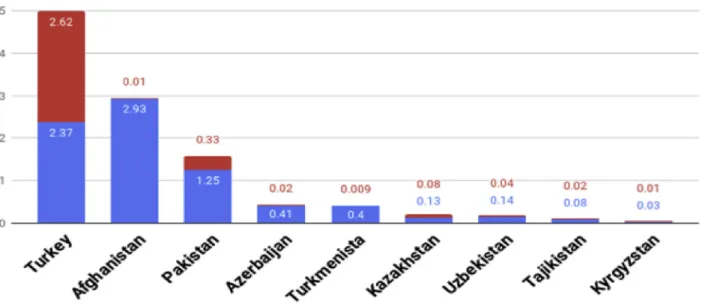
whereas exports stood at 8.42 billion m3, the key trade partners being Turkey, Azerbaijan, Turkmenistan and Armenia.Figs. 1–3provides the schematic of the dynamic of natural gas dynamics. For instance,Fig. 1 shows the persistent trend in the last 2-3 decades of production and consumption of natural gas. SubsequentlyFigs. 2 and 3also renders a pictorial display of top natural gasflaring nations in the world and net trading partners with Iran.
The adoption of NG as a feasible alternative to other fossils fuels has resulted in an increase in Iran's domestic consumption of NG. This crement is also noticeable in exports as the country's NG exports in-creased byfive-fold to 60 billion m3by 2014 as outlined byIran Oil Ministry Annual Bulletin, 5th edition. This increase in NG consumption is a result of the combination of the following factors: reduction in the domestic supply price of NG, wasting energy technologies, in-appropriate and abundant use of NG. This consumption situation raises certain issues; on one hand, one may assume that increased NG con-sumption will produce a cleaner environment and birth economic
prosperity, while on the other hand however, numerous researchers have suggested that in general, resource extraction often crowds out other economic activities, especially manufacturing, and reduces the growth impact of other sectors of the economy (Mankiw et al., 1992; Sachs and Warner, 2001). The above assertion is known as Dutch dis-ease hypothesis. Thus, it pertinent to examine how NG affects the economic growth of Iran. Also, while NG demand may be able to affect economic growth, economic growth may also have effect on NG de-mand, as the strength of an economy can influence the energy market. For example, during periods of boom, increases in demand for goods and services may cause increases in NG consumption. Thus, the need to underpin the directional causality flow between NG
consumption-Fig. 1. Iran Dry natural gas production and consumption Source: United States Energy Information Administration (2018)
Fig. 2. Top natural gasflaring countries
Source: U.S. Energy Information Administration, based on OPEC Annual Statistical Bulletin (2015)
economic outputs is pertinent and timely.
Recently, there has been growing interest in examining the linkage between economic growth and NG consumption. Studies on this issue have however produced contradictory empirical outcomes. These con-tradictions in extant literature may be as a result of the bivariate econometric frameworks mostly adopted in past studies. A majorflaw of bivariate models is that they suffer from omitted variable bias (model misspecification) and for this reason, their estimation outcomes are spurious. The implication is that the policy implications from such studies are unreliable (Dolado and Lutkepohl, 1996). There is thus a need to incorporate additional important variables with relatively high explanatory powers. Hence, scholars such as (interalia Apergis and Payne, 2010;Kum et al., 2012), among others have studied the theme under consideration in multivariate framework using diverse econo-metric approaches.
Against the above highlighted premise that this study explores the interaction between consumption of natural gas-economic growth nexus by extending the bi-variate framework by incorporation of im-portant variable to make multivariate. The addition of our study to the frontiers of knowledge is in four-fold; (i) In terms of scope, we augment the NG-economic growth nexus with real grossfixed capital formation (GFCF) to ascertain the role of capital in economic output and also with oil rent seeking for Iran given the pivotal role oil plays in Iranian economy an area which has not been properly documented in the lit-erature. Also, the present study also explore the role of non-oil GDP on NG consumption in Iran economic output given the peculiarity of our case study. The Iranian economy has suffered from war and western sanction before the 1990s so it pertinent to see if such episodes plays out on the current empirical discourse (Amadeh et al., 2009;Hafeznia et al., 2017;Akadiri and Akadiri, 2018). (ii) In terms of methodological advancement, because most economic and financial datasets are pla-gued with possible break dates we account for structural break in our econometric analysis. The need to account for possible break(s) dates are pertinent, otherwise obtain coefficient estimates will be inconsistent and unreliable for policy analysis. (iii) This study applies estimation techniques such as Zivot and Andrews (1992)unit root to detect the unit root/stationarity traits of variables under consideration. (iv) For cointegration relationship, we utilize Pesaran's auto regressive dis-tributive lag (ARDL) methodology and the newly advancedBayer and Hanck (2013) combined cointegration test as complementary to Pe-saran's test while we apply Toda-Yamamoto-Granger causality test
(1995) a modified Wald methodology (MWALD) which is known to render more robust results than the conventional Granger causality test is adopted to detect the direction of causality to explore the causality flows between the variables under review.
The rest of the current study proceeds as; section-2 provides a brief review related studies on NG-economic growth. Section-3 dwells on the methodological construction and data while section-4 concentrates on empirical findings and discussion. Finally, the study summary (con-clusions) and possible policy direction are rendered in section-5.
2. Theoretical background
A few theoretical studies have been documented formally that model a direct connection between energy and economic growth, en-ergy and environment. The extant empirical literature on the theme cut across single country, cross country and panel analysis. We set off by briefly discussing the theoretical foundation. Subsequently, empirical studies that outline the transmission mechanism that explains the en-ergy-income nexus. For this particular study, the incorporation of oil rent and capital to economic growth is explained.
The quest for economic growth seems the most pertinent issues for most if not all economies across the globe. Thus, the need to identify growth indicators is key for government administrators and policy-makers. There exist a large body of theoretical studies on the economic growth, majority rely on the well-known Solow growth model. The Solow growth model outlined that a substantial level of labour and capital accumulation with right level of technology known as the“Slow residual” explains economic growth. Over the years the conventional Solow growth model has been augmented with other variables like energy use, tourism, population and other demographic indicators (Soytas and Sari, 2009).
The study ofKraft and Kraft (1978)empirically serves as the bed-rock in energy literature when considering the relationship between income and energy consumption. The study serves as an invitation to several other studies in the energy economics literature. It is fromKraft and Kraft A, 1978that this study establishes an interaction between economic growth and energy consumption for the United State. Further motivation for this present study is hinge on the theoretical framework developed by (Dietz and Rosa, 1994;York et al., 2004) popularly re-ferred to as Stochastic Impacts by Regression on population, Affluence, and Technology (STIRPAT).
Fig. 3. Top trading natural gas importing and exporting countries with Iran Source: IEA (2018)
Iran being a world leader in the NG exportation and major consumer domestically, with lot of revenues derived from NG can lead to an in-crease in accumulation of foreign exchange reserves. Where there is a considerable improvement in the terms of trade, this will have a ripple effect on the appreciation of the real exchange rate. This will also translate in the short run to economic growth.
The transmitting mechanism by which energy consumption trans-lates into economic growth is seen from the accrual from the revenues generated from the proceeds of NG consumption. Increase from this revenue is used both for investment in the public infrastructure archi-tecture as well as consumption. In the work of Basher and Fachin (2013), long run interaction is established to exist between savings and investment. In recent times, there been a drift from household con-sumption to the industrial sector given the adoption of new technolo-gies for exploration and exploitation of NG. These new technolotechnolo-gies in form of high efficiency low emission (HELE) approach will increase the industrial consumption of NG in Iran in the coming years. More so, government intervention in terms of pipeline installation and subsidies has also encourage private sector investment in no more measure. This finding helps to relax the constrain of low domestic savings which is usually encountered by private investment, so higher income from the NG revenues induces higher savings thereby increase in investment and accumulation of capital which is key in expanding the economic ac-tivities in the domestic economy (Ramey, 2011;Esfahani and Yousefi, 2017).
Numerous studies in recent years investigating the relationship be-tween energy consumption (including both renewable and nonrenew-able sources) and economic growth abound in the energy literature. Payne (2010) and Ozturk (2010) in their comprehensive review of various literatures on NG and economic growth nexus basically sum-marized four hypotheses that are testable.1
There are limited papers in the literature with regard to causal re-lationship between NG consumption and economic growth. This review will explore it categorically to ascertain the extent to which gap exist. First category explores studies that have deduce causality between these variables using cointegration technique. Second category con-siders bivariate studies which have employed causality tests. Third category explores the trivariate approach while still employing the causality tests. The last category while building on the shortfalls of previous categories, uses multivariate series to implement the causality tests. Beginning with thefirst category,Lee and Chang (2005)studies have applied the cointegration techniques to examine the relationship between NG and economic growth. These studies used Johansen (1988),Hansen (1992), andGregory and Hansen (1996)test of coin-tegration to examine for the period 1954–2003 relationship between NG consumption and economic growth. The test results revealed causalityflow from NG consumption to real GDP using the weak exo-geneity as a notion of long run causality in a cointegration system.
According toZamani (2007)investigated the relationship between the Iranian economy and NG consumption covering the period from 1967 to 2003. Evidence from the studies showed bidirectional re-lationship between NG consumption and GDP. Similar studies in Taiwan was conducted by Hu and Lin (2008)usingHansen and Seo (2002)cointegration test to investigate the relationship between real GDP and NG consumption. The result supported and confirmed feed-back hypothesis for Taiwan. In Pakistan for the period 1972–2007, Khan and Ahmad (2008) usedJohansen (1988)along withJohansen and Juselius (1990)tests to examine the relationship NG consumption per capita, gas price and real GDP per capita. Conservative hypothesis was ascertained and confirmed from the analysis. Isik (2010) in-vestigated the relationship between NG consumption and economic growth for the period span of 1977–2008 in Turkey. The result showed
a positive influence of NG consumption by the economic growth in the short run whereas in the long run negative relationship was observed. Considering various reviews made by scholars as contribution to the body of knowledge on this subject, there seem to be a major weakness of applying cointegration tests to determine causality direction without including Granger causality formally. Nevertheless, cointegration ex-istence does not necessarily specify causality direction.
Certain bivariate studies have applied series of causality tests to deduce that there exists causal relationship between NG consumption and economic growth.Yu and Choi (1985)in attempt to determine the direction of causality in UK, US and Poland deployedSims (1972)and the result showed causalityflowing economic output (GDP) towards NG consumption, whereas in the case of US and Poland there was no causality established among the variables. Investigating the relation-ship between NG consumption and economic growth in Pakistan drove Siddiqui (2004)to useHsiao (1981)for the period span 1970–2003. No causality was found among the variables as revealed by the results. A case of single causality was observed to be flowing from NG con-sumption to economic output as investigated by Yang (2000)in his studies seeking to establish causality between utilization of gas and economic growth in Taiwan for the period of 1954–1997.
Adeniran (2009) deployed Sims (1972) tests of causality to in-vestigate the causal relationship in Nigeria from 1980 to 2006. Caus-ality was observed from the results toflow from the real GDP to NG consumption.
Furthermore,Payne (2010)for the period 1949–2006 in the US. The study investigated causal relationship between economic growth and NG consumption. Positive causality that is a directional causality flowing from economic growth towards NG consumption was the out-come of study. Also, in a different bivariate study by Zahid (2008), where three countries (India, Bangladesh and Pakistan) where in-vestigated with regards to causality relationship from 1971 to 2003. One direction causality flowing from NG consumption was observed from the results to the economy in Bangladesh, whereas no causality was demonstrated for India and Pakistan.Lim and Yoo (2012)using quarterly data from 1991 to 2008 examined causal relationship be-tween NG consumption and economic growth in Korea for both short and long run. Evidence of double-sided Granger causality was reported from the result between NG consumption and economic growth.Das et al. (2013)examined the interaction or association existing between NG consumption and economic growth from 1980 to 2010 in Bangla-desh. Results from this study established that NG consumptionflow to real GDP in the long run and it is one way with Granger causality test. Similar study byBildirici and Bakirtas (2014)explored the relationship between economic growth and NG consumption among the various types of energy available for countries including Russia, Turkey and Brazil. Evidence from the tests result showed feedback causality re-lationships between economic growth and NG consumption for the countries under study.Pirlogea and Cicea (2012)also considered the causal relationship between NG consumption and economic growth per capita for the period 1990–2010 in Romania and Spain. Evidence from test results usingGranger (1969)revealed causal relationshipflowing from NG consumption towards economic growth in Spain, whereas in Romania there was no causal relationship established.
More recently,Solarin and Ozturk (2016)assessed the causal re-lationship between NG consumption and economic growth in a panel of OPEC members, and theirfindings revealed a feedback relationship. However, evidence obtained when member countries were examined individually was different. There was evidence of growth hypothesis in countries like Iraq, Kuwait, Nigeria and Saudi Arabia, whereas the conservative hypothesis held in other member countries like Algeria, Iran, the United Arab Emirates and Venezuela. Furthermore, the neu-trality hypothesis was evident in the case of Angola and Qatar, while Ecuador was the only country with feedback hypothesis.
In the study on Malaysia bySolarin and Shahbaz (2015), the feed-back hypothesis was confirmed. Studies on the theme for Iran are
1For brevity, interested readers can see the literature studies of Payne (2010) andOzturk (2010)for more insight on the testable causality hypotheses.
limited. However, Zamani (2007), using the vector error correction model (VECM), examined disaggregated energy consumption estimates from 1967 to 2003 and found a long run bidirectional causality re-lationship stemming from economic growth to NG consumption. More recently,Esen and Oral (2016)andHafeznia et al. (2017)affirmed the significant contribution of NG to economic growth in the various in-vestigated countries.
Kum et al. (2012)examined relationship between NG consumption and economic growth in the G-7 countries (US, UK, Japan, Italy, Ger-many, France and Canada) for the period 1970–2008. With control for capital in the model, test results showed causality flowing from NG consumption towards economic growth for Italy, whereas in the case of UK no causality is established from NG consumption to economic growth. From the results, it also revealed US, Germany and France were observed to have bidirectional causality whereas for Canada and Japan no causal relationship was established. Lotfalipour et al. (2010) in-vestigated into causal relationships between economic growth, carbon emissions and fossil fuels consumption for Iran during 1967–2007 period. Proxying with NG consumption, results revealed unidirectional Granger causalityflowing from NG consumption to GDP.Saboori and Sulaiman (2013)investigated into the relationship between NG con-sumption and economic growth in Malaysia from 1980 to 2009. In the short run, evidence is observed from the result showing unidirectional causality flowing from NG consumption to economic growth. In the case of long run from the same result, bidirectional causality is evident
between NG consumption and carbon emissions, economic growth and NG consumption.
The problem of omission of important variable is minimized using the trivariate approach, through addition of extra variable is of little effect to resolve this problem. This has necessitated recent studies to adopt the use of multivariate framework to resolve this issue.Shahbaz et al. (2013c)examined the relationship in Pakistan covering the period from 1972 to 2010. Export, capital and labor were added in the mul-tivariate model. Variance decomposition analysis was carried to es-tablish causal relationshipflowing from the NG consumption to eco-nomic growth.Apergis and Payne (2010)investigated the relationship between NG consumption and economic growth for the period of 1992–2005 using panel of 67 countries. This study included capital formation and labor force to the model. With the use of heterogenous panel cointegration, there was evidence of bidirectional causality and long run relationships between economic growth and NG consumption. According to the studies ofFarhani et al. (2014)who explored the role of NG consumption withfixed capital formation and trade over the specified period 1980–2012 on Tunisia economic growth. Result re-vealed bidirectional causal relationship between NG consumption and economic growth. Ighodaro (2010) examined the link between NG utilization and economic growth in Nigeria for the period 1970–2005. With the inclusion of broad money and health expenditure variables into the model, evidence from the result revealed unilateral causal re-lationship as well as long run link flowing from NG utilization to
Table 1
Summary of literature on Natural gas-economic growth nexus.
Authors and Year Time Region Methodology Empirical Finding
Akadiri and Akadiri (2018) 1980–2013 Iran ARDL, TY Y x NG
Hafeznia et al. (2017) N/A Iran Descriptive statistics, Graphs NG↔ Y
Esen and Oral (2016) N/A Iran, Russia, Qatar, Turkmenistan Descriptive statistics, Graphs
NG↔ Y
Furuoka (2016) 1980–2012 China ARDL,GC,TY NG→ Y
Solarin and Ozturk (2016) 1980–2012 OPEC member countries Panel GC NG↔ Y
Balitskiy et al. (2016) 1997–2011 EU-26 Panel cointegration NG↔ Y
Destek (2016) 1991–2013 OECD countries FMOLS, DOLS
Panel VECM
NG↔ Y
Shahiduzzaman and Alam (2014) 1970–2009 Australia ARDL NG↔ Y
Bildirici and Bakirtas (2014) 1980–2011 Brazil, Russia and Turkey ARDL, JML,GC NG↔ Y
Solarin and Shahbaz et al. (2015) 1971–2012 Malaysia BH,ARDL, VECM, NG↔ Y
Rafindadi and Ozturk (2015) 1971–2012 Malaysia ARDL,BH,GC NG↔ Y
Ozturk and Al-Mulali (2015) 1980–2012 Gulf Cooperation Council (GCC) Countries
Pedroni cointegration test NG↔ Y
Dogan (2015) 1995–2012 Turkey VECM, GC NG↔ Y
Farhani et al. (2014) 1980–2010 Tunisia ARDL, TY NG↔ Y
Saboori and Sulaiman (2013) 1980–2013 Malaysia ARDL, JML, GC NG↔ Y
Shahbaz et al. (2013b) 1972–2010 Pakistan ARDL,JML,GC NG→ Y
Das et al. (2013) 1980–2010 Bangladesh JML,GC Y→ NG
Kum et al. (2012) 1991–2008 Korea GC NG↔ Y
Lotfalipour et al. (2010) 1967–2007 Iran TY NG→ Y
Apergis and Payne (2010) 1992–2005 67 Countries Pedroni cointegration NG↔ Y
Ighodaro (2010) 1970–2005 Nigeria VECM, JJ NG→ Y
Isik (2010) 1977–2008 Turkey ARDL NG↔ Y
Amadeh et al. (2009) 1973–2003 Iran ARDL, VECM NG← Y
Reynolds and Kolodziej (2008) 1928-1987,1988–1991,1992–2003 Soviet Union GC NG→ Y
Hu and Liu (2008) 1973–2003 Taiwan VECM NG← Y
Sari at al. (2008) 2001–2005 US ARDL, VECM NG← Y
Zamani (2007) 1967–2003 Iran JML, VECM NG↔ Y
Lee and Chang (2005) 1954–2003 Taiwan JML, WE NG→ Y
Siddiqui (2004) 1970–2003 Pakistan ARDL, HGC(Hsiao's Granger Causality
Test)
NG x Y
Fatai et al. (2004) 1960–1999 New Zealand and Australia ARDL, JML, TY Y x NG
Aqeel and Butt (2001) 1955–1996 Pakistan GC Y x NG
Yang (2000) 1954–1997 Taiwan GC NG→ Y
Yu and Choi (1985) 1947–1974 US, UK GC NG← Y
Note: NG- Natural gas consumption, Y- economic growth. Where NG→ Y means one-way causality from NG consumption to economic growth and Y → NG is from economic growth to NG consumption. Y↔ NG depicts a feedback Granger causality and Y x NG denotes neutrality hypothesis where there is no causal interaction between NG and Y. Also inTable 1above N. A-not applied. The following abbreviation tests are rendered as Autoregressive Distributed Lag Model to Cointegration (ARDL), Granger Causality (GC). Also the (JML) mean Johansen's Maximum Likelihood technique, Johansen Juselius cointegration(JJ), Vector Error Correction Model(VECM) Bayer and Hanck cointegration test(BH) and Toda and Yamamoto causality tests (TY) respectively.
economic growth.
While research on energy-economic growth is quite large, there is only a limited number, which tested the income-energy nexus through the channel of oil rent and natural gas consumption with each pro-viding an inconclusive results. The studies of Emami and Adibpour (2012)clearly outlined the pivotal role of oil rent on economic growth in Iranian economic growth. As a positive shock on oil rent translate into increased economic output. On the contrary, a negative shock from oil rent birth decline in output level. The above position of oil rent driving economic growth is also consistent with the study ofMehrara (2007)for top oil exporting countries. Also, the inclusion of low-cost capital as substitute to labor in connection with expansionary and re-distributive policies results in fast wage rate (Esfahanin and Yousefi, 2017). At the same time as the country's oil boom revenue rises it causes the real exchange rate to rise, this induces the demand for domestic production of tradable to shift. This will cause total factor productivity and labor productivity to increase. Thus, it on the above premise the present study seek tofill these identified gap. Where little or less at-tention has been documented. The current study revisit the natural gas-led growth nexus with a new perspective by the inclusion of oil rent and non-oil GDP, capital to make more a more robust theoretical and em-pirical contribution.
Table-1 below renders summary of studies on the theme under consideration with diverse estimation techniques for bloc or country-specific cases.
3. Methodological construction 3.1. Data
To investigate the interaction between NG consumption and eco-nomic output in Iran, a multivariate framework which also includes real gross capital fixed formation (RGFCF) (constant 2010) as proxy for physical capital is adopted. The data for real gross domestic product (RGDP) (constant 2010) as well as Non-oil GDP that disentangle impact of oil on economic growth as also account for the model construction. Real gross capital formation and carbon dioxide emissions in Kt. Oil rent was also incorporated into the study to account for the significant role of oil revenue in the Iranian economy. The data were sourced from World Bank Development Indicators (https://data.worldbank.org/ in-dicator), while data for NG was retrieved from the U.S Energy Information Administration database (EIA, 2018). Oil rent and Non-oil GDP were sourced from the Thomson router DataStream on a quarterly basis from 1990Q1 to 2017Q4 for the econometric analysis.2
The study's empirical path is as follows; (i) Unit root analysis through traditional non-stationarity tests of Augmented Dickey and Fuller, 1981andPhillips and Perron (1988)tests and added to capture for a breakpoint in stationarity analysis is theZivot and Andrews, 1992. The aforementioned test will be employed to explore maximum in-tegration order of the interest variables as well as aid in avoiding I(2) variables. (ii) The estimation of cointegration among the series was achieved via thePesaran et al. (2001)Bounds testing complemented with newly advanced combined cointegration test ofBayer and Hanck (2013). Finally, Granger causality procedure is estimated to observe the causal relationships between the variables.
3.2. Model framework
The functional relationship for our study draws empirical strength fromSolarin and Shahbaz (2015)andSolarin and Ozturk (2016), given as: = GDP f NGC GFCF OR( , , ) (1) = + + + + LnGDPt α β LnNGC1 t β LnGFCF2 β LnOR3 εt (2) = Nonoil GDP_ f NGC GFCF OR( , , ) (3) = + + + + LnNonoil GDP_ t α β LnNGC1 t β LnGFCF2 β LnOR3 εt (4)
Logarithm transformation is carried out on equation (1) to also achieve homoscedasticity.
Here,αrepresents constant whileβ β1, 2,β3are partial slope parameter. The apriori expectation of the abovefitted models aligns with theory and empirical support. The expectation for β1> 0. That is in con-firmation of the natural gas led-growth hypothesis. As natural gas, consumption contributes to economic growth.β2> 0. This implies that capital accumulation play a positive role in Iran economy as supported by earlier study ofAkadiri and Akadiri (2018). Finally, the expected sign forβ3 is ambiguous as it could be either positive or negative de-pending on the time and economic structure. Empirical studies have reported mixed outcome. As a negative sign is supported by the war-time, sanctions, political instability and corruption witnessed in the energy sector with rest of the world in Iran also contributed. As oil revenue decline and lot of trading partners found substitute energy, that is, alternative and other trading hub also had it toll on the country economy see (Mehrara, 2007; Emami and Adibpour, 2012). On the contrary, a positive sign is also visible if all earlier mentioned menace are control for, especially corruption in the energy sector that has crippled economic progress over the years in Iran (World Bank, 2017).
3.3. Stationarity test
The need for unit root and stationarity test in time series analysis is pertinent among variables. This is essential to appraise the variables order of integration. This is in quest to avoid spurious regression. The econometrics literature has well documented numerous tests, among which are the AugmentedDickey and Fuller, 1981,Phillips and Perron (1988)andElliott et al., 1992test. A shortcoming of the conventional unit root tests highlighted above is that they fail to account for struc-tural break(s). These tests offer invalid and inconsistent estimates in presence of structural break(s) dates. It is however a well-known fact that most macro finance and economic datasets are plagued with structural breaks reflecting economic episodes and events. Thus, our study complements the conventional unit root tests with Zivot-Andrews unit root test. The Zivot-Andrews unit root test is reputed to account for a single structural break.
The Formula for ZA test models are given below as:
∑
= + + − + + +
= −
ΔYt α α t θYt γDUt ξ ΔY ε
i k i t i t 1 2 1 0 (5)
∑
= + + − + + + = −ΔYt α α t θYt φDTt ξ ΔY ε
i k i t i t 1 2 1 0 (6)
∑
= + + − + + + + = −ΔYt α α t θYt γDUt φDTt ξ ΔY ε
i k
i t i t
1 2 1
0 (7)
where the dummy variable DUtshows the shift that occurs at each point
of possible breaks at either intercept, trend or both intercept and trend. The ZA unit root test has a null hypothesis of (unit root), meaning,
H0:θ> 0 against an alternative (stationarity), H1:θ< 0. That is, failure to reject H0 means the presence of unit roots while and rejection implies stationarity.
3.4. Cointegration test
The econometrics literature has well documented several proce-dures for cointegration relationship among interest series. Two series are said to have a long-run relationship (cointegrated), if there is
2Data interpolation technique available at E-views 10is employed to convert all annual data into quarterly frequency. Our study leverages on the study of (SeeShahbaz and Lean, 2012).
somewhat linear combination among such series. Examples of the available cointegration tests areEngle and Granger, 1987, Johansen and Juselius (1990), Philips and Ouliaris (1990), Johansen (1991). Others includeGregory and Hansen (1996)andCarrion-i-Silvestre and Sansó (2006). However, all aforementioned tests have varying conclu-sions ranging from cointegration to non-cointegration null hypothesis. Bayer and Hanck (2013)recently advanced cointegration test provides more robust results by the amalgamation of different individual test statistics premised on the test Engle and Granger (1987), Johansen (1991), Boswijk (1995)andBanerjee et al. (1998) tests. The Fishers’ formulae of the combined Bayer and Hanck (2013)test is provided below as outlined in a study byShahbaz et al. (2016).
− = − +
EG JOH 2[ln(PEG) (PJOH)] (8)
− − − = − + + +
EG JOH BO BDM 2[ln((PEG) (PJOH) (PBO) (PBDM) (9) here, PEG,PJOH,P andPBO BDMare the corresponding probability values of
the various individual cointegration tests.
3.5. Autoregressive distributive lag (ARDL) approach
Furthermore, to reinstate the robustness of cointegration between NG consumption and economic output, gross fixed capita formation, and carbon dioxide emissions, we leverage the ARDL bounds testing technique that offers more robust and efficient estimates on the case of small sample size when compared to other conventional cointegration tests. Furthermore, the ARDL bounds test reports both short and long run dynamics of the fitted regression alongside the error correction model term (ECT) simultaneously. In addition to the above-mentioned merits, the technique is also useful in case of unknown order of in-tegration of series. That is, the technique can be employed irrespective of whether the series are I(0) or I(I), but not 1(2). The model is esti-mated in the bounds test framework via the unrestricted error correc-tion model where all variables are taken as endogenous. The UECM is estimated as:
∑
∑
∑ ∑
= + + + + + + + − = − = − = = − ΔY μ μ t λ y θ v γ ΔY ω ΔV ΨD ε t i N it j p j t j i N j P ij it j t t 0 1 1 1 1 1 1 1 1 1 (10)whereVtdenotes vector; Dt accommodates for structural break in the
framework as an exogenous variable. The test has a null of no coin-tegration with the bounds test, which is computed using F-statistics. The decision rule houses three scenarios. First, if the computed F-sta-tistics is greater than upper bounds of the critical values reported, the null is rejected. Second, if F-statistic lies with both lower and upper bounds, the decision is inconclusive and third, scenario state that if F-statistic lies below the upper bounds, it a case of no cointegration. The hypotheses for the bounds test are specified below as:
H0:φ1=φ2= …. = φk+2= 0
H1:φ1≠ φ2≠ …. ≠ φk+2≠ 0
3.6. Cointegration estimation equation
Cointegration regression is necessary after establishing long-run association among series. Several of such test abound in the literature, among such are fully modified ordinary least squares (FMOLS) ad-vanced byPhillips and Hansen (1990), dynamic ordinary least squares (DOLS) byStock and Watson (1993). Others includePark's (1992) Ca-nonical Cointegration Regression (CCR). These cointegration estimation methodology offers robustness check of estimated regression as well as they offers reliable results in cases of small sample sizes they efficient.
3.6.1. FMOLS
When cointegration exists among series integrated atfirst order ‘I (1)’, (FMOLS) estimation offers optimal cointegrating regression esti-mates (Phillips and Hansen, 1990; Hansen, 1995; Phillips, 1995; Pedroni, 2001a,b). The method is able address issues of endogeneity and autocorrelation and still render robust estimates. Given the equa-tion below:
= + + ∀ = … = …
Yi t, αi β Xi i t, εi t, t 1, , ,T i 1, ..N (11) Allowing for Yi t, and Xi t, are cointegrated with slopesβi, whereβi
may or may not be homogeneous across i. Hence, the equation be-comes:
∑
= + + + ∀ = … = =− − Yi t αi β Xi i t γ ΔX ε t 1,2, , ,T i 1, ..N k K K i k i t k i t , , , , , i i (12) We reflectξi t, =(ˆ , Δεi t, Xi t,) and = ⎡⎣ ∑ ∑ ⎤⎦ →∞ = = Ωi t limE ( ξ )( ξ ) T T i T i t i T i t , 1 1 , 1 ,as the long covariance. Here Ωi=Ωi0+Γi+Γ´i; The simultaneous
covariance is depicted asΩi0also the weighted sum of autocovariance is
Γi. Thus, the equation of the FMOLS is rendered as:
⎜ ⎟
∑
⎡
⎣
⎢ ∑
⎛
⎝
∑
⎞
⎠
⎤
⎦
⎥
= ⎛ ⎝ ⎜ − ⎞ ⎠ ⎟ − − ∗ = = − = ∗ β N X X X X Y T ˆ 1 ( ‾ ) ( ‾ ) FMOLS i N i T i t i i T i t i i t γ 1 1 , 2 1 1 , , ˆi (13) where = − − = + − + ∗ ∗ Y Y Y Ω Ω X and γ Γ Ω Ω Ω Γ Ω ‾ ˆ ˆ Δ ˆ ˆ ˆ ˆ ˆ ( ˆ ˆ ). i t i t i i i i t i i i i i i i , , 2,1, 2,2, , 2,1, 2,1, 0 2,1, 2,2, 2,2, 2,2, 0 (14) 3.6.2. DOLSThe long-run regression estimator of fully modified dynamic least square can be substituted with the dynamic ordinary least squares, given her merit over the FMOLS (Saikkonen, 1991;Stock and Watson, 1993). The DOLS technique is built to be asymptotically efficient esti-mator as well as eliminate feedback in the cointegrating system. Econometrically, the approach estimation process contains the coin-tegrating regression which possess both lags and leads, considering the orthogonality in the cointegrating equation error term:
∑
= + + + =− + Yt αi β X´t D D γ´t ´ Δ ´X ρ v j q r t j t 1 1 1, (15) The differenced regressors with lag and lead of q and r respectively, absorbs all the long-run correlation between (ν1t and ν2t) while the least-square estimates ofθ = (β′, γ′)' houses asymptotic distribution similar to canonical cointegration regression and fully modified or-dinary least squares.3.6.3. CCR
The Canonical Cointegration Regression (CCR) is unique by cir-cumventing bias of second-order a short coming of the ordinary least squares (OLS) estimator by transformation of the variables. The cov-ariance matrix form of the long-run estimator is rendered as:
= ∑ ∑ = ⎡ ⎣ ⎢ ⎤ ⎦ ⎥ →∞ = = Ω u u Ω Ω Ω Ω limn E t ( ) ( )´ n t t n t 1 1 11 12 21 22 (16)
whereΩ can be represented as follows:
∑
= + + Ω Γ Γ´ (17) and∑
= →∞∑
= limn E (u u´ ) t n t t 1 (18)∑ ∑
= → = − = + − Γ limn E E(u u´ ) n k n t k n t t k 1 1 1 1 (19) ∩ = ∑ + = ∩ ∩ = ⎡ ⎣ ⎢ ∩ ∩ ∩ ∩ ⎤ ⎦ ⎥ Γ ( 1, 2) 11 12 21 22 (20)the transformed series is obtained as:
∑
= − − ∩ ∗ Y Y u 1 ( )´ t t t 1 2 2 (21)∑
= − − ∩ ∗ Y Y u 1 ( )´ t t t 2 2 2 (22)∑
⎜ ⎜ ⎜ ⎟ ⎟ = −⎛ ⎝ − ⎛ ⎝ ∩ +⎛ ⎝ ⎞ ⎠ ⎞ ⎠ ∗ − Y Y β Ω Ω u 1 0, , ´ ´ t t t 1 1 2 12 221 (23) where CCR acquires the following form:= + + ∗ ∗ ∗ Y1t β´ Y2t u1t (24) = − ∗ − Y1t u1t Ω12, Ω221u2t (25)
Equation-24the OLS estimators share the same fashion as the ML estimation. The long-run correlation of y1t and y2t caused asymptoti-cally endogeneity were circumvented for by variables transformation. The asymptotic bias issue because of cross-correlation between (u1tand
u2t), were addressed in Equation-25 with the transformation of the
variables.
3.7. Causality approach
The traditional regression does not imply causal interaction. Thus, there is need for causality test to probe directional causality between variables. This is necessary, given the inherent insight that can be gleaned from such estimations by policy makers and stakeholders in general. Our study employs the Granger causality approach as the primary means of detecting the predictability power that exists among the variables. When we say variable X Granger causes Y, it implies that variable X and its past realizations are good predictors of variable Y. A general model specification for the bivariate (X, Y) Granger causality test is expressed thus:
= + − + − +
Xt γ0 γ X1 t 1 γ Y2 t 1 εt (26)
= + − + − +
Yt γ0 γ Y1 t 1 γ X2 t 1 εt (27)
Inequation-26, the null hypothesis that X doesn't Granger cause Y is tested against the alternate hypothesis that X Granger causes Y. The hypotheses are similarly stated forequation-27. It is also worthy of note that the causal relationships can take one of the following forms; uni-directional (meaning from X to Y or vice versa), biuni-directional (implying feedback relationship from both ends) and neutrality (implying no ca-sual interaction between the variables).
3.7.1. Toda-Yamamoto Granger causality methodology
The fact that conventional regression does not connotes causality interpretation. This necessitates the need to estimate causality test. The current study relies on the modified Wald stat (MWALD) Toda-Yamamoto (1995)causality test to detect theflow of causality for the selected variables under consideration. The Toda-Yamamoto (TY, here after) is preferred to the traditional Granger causality because The TY possesses some distinct traits relative to conventional Granger causality test. The TY can be conducted regardless of cointegration relationship among variables. Also, there is no precondition of stationarity proper-ties of variables to be either integrated of order 1 or stationary at levels. However, the variable(s) should not integrated of order 2. The TY methodology is conducted on a VAR settings, with a known VAR (k + dmax). Where dmax denotes the maximum order of integration of the variables and K represents the optimum lag order as suggested by
appropriate lag selection criterion. The present study employs a mul-tivariate VAR (k + dmax) model which encompasses economic growth (GDP), oil rent, Non-oil GDP and Natural gas consumption. The model specification is rendered below as:
= + ∑ + ∑ + ∑ + ∑ + ∑ + ∑ + ∑ + ∑ + = − = + − = − = + − = − = + − = − = + − GDP ϕ ϕ GDP ϕ GDP δ GFCF δ GFCF β NGC β NGC ξ OR ξ OR ε ln ln ln ln ln ln ln ln ln k n k t k r md r t r k n k t k r m d r t r k n k t k r m d r t r k n k t k r m d r t r t 0 1 1 1 2 1 1 1 2 1 1 1 2 1 1 1 2 1 max max max max (28) = + ∑ + ∑ + ∑ + ∑ + ∑ + ∑ + ∑ + ∑ + = − = + − = − = + − = − = + − = − = + − NGC β β NGC β NGC ϕ GDP ϕ GDP δ GFCF δ GFCF ξ OR ξ OR ε ln ln ln ln ln ln ln ln ln k n k t k r m d r t r k n k t k r m d r t r k n k t k r m d r t r k n k t k r m d r t r t 0 1 1 1 2 2, 1 1 1 2 1 1 1 2 1 1 1 2 2 max max max max (29) = + ∑ + ∑ + ∑ + ∑ + ∑ + ∑ + ∑ + ∑ + = − = + − = − = + − = − = + − = − = + − GFCF δ δ GFCF δ GFCF ϕ GDP ϕ GDP β NGC β NGC ξ OR ξ OR ε ln ln ln ln ln ln ln ln ln k n k t k r md r t r k n k t k r m d r t r k n k t k r m d r t r k n k t k r m d r t r t 0 1 1 1 2 1 1 1 2 1 1 1 2 1 1 1 2 3 max max max max (30) = + ∑ + ∑ + ∑ + ∑ + ∑ + ∑ + ∑ + ∑ + = − = + − = − = + − = − = + − = − = + − OR ξ ξ OR ξ OR δ GFCF δ GFCF ϕ GDP ϕ GDP β NGC β NGC ε ln ln ln ln ln ln ln ln ln k n k t k r m d r t r k n k t k r m d r t r k n k t k r md r t r kn k t k r m d r t r t 0 1 1 1 2 1 1 1 2 1 1 1 2 1 1 1 2 4 max max max max (31) where GDP, NGC, OR and GFCF are all expressed in section3.1. Also,
ε1t,ε2tandε3trepresent stochastic terms forfitted models. Where k
de-notes the optimal lag order. By using the standard Chi-square statistics, Wald tests are employed to thefirst n coefficient matrices.
4. Empiricalfindings and discussions
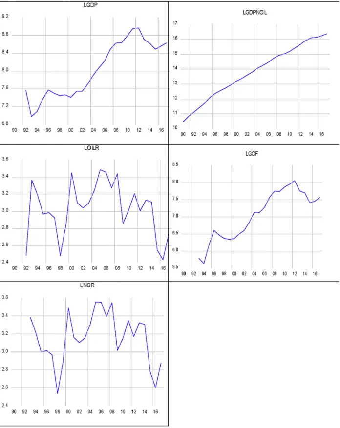
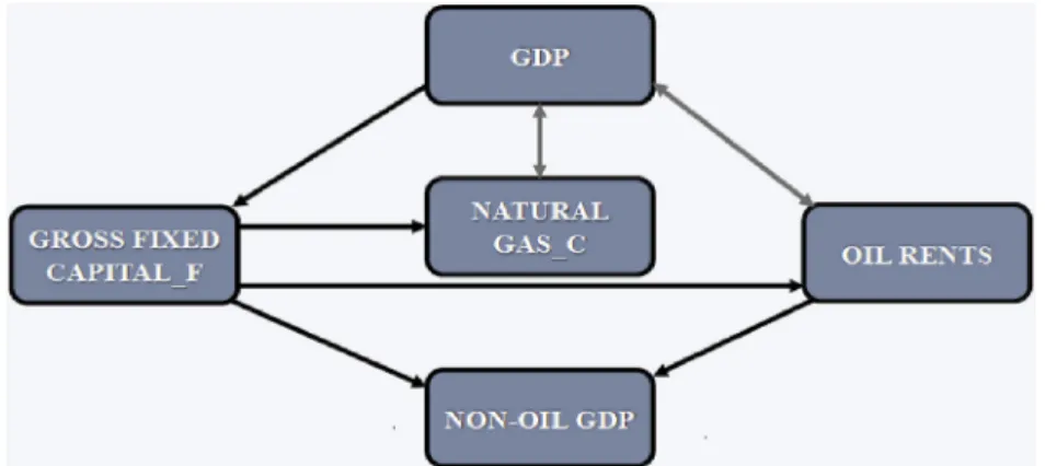
In time series estimations, it is essential to have a visual plot of the variables in order to have a glimpse of how the dataset fares.Fig. 4 below shows the variables under review. FromFig. 1, it is conspicuous that there exists noticeable structural break(s). Thus, our study mod-elled for such break(s) in the estimation section.Table 2reports the basic summary (descriptive) statistics and correlation matrix analysis in the panel.Table 2shows that all series investigated are normally dis-tributed as reported by the Jarque-Bera probability which is desirable. Also observed is obvious significant disparity between the minimum and maximum over the period investigated, which is worth further investigation. The correlation matrix is also reported at the bottom of Table 2. The correlation results show a positive association between NG intake and economic output (GDP) for the study area, which is desirable and expected for Iran, being a net exporter of NG. Also revealed is significant positive synergy between RGFCF and economic growth, thus suggesting the key role of real gross capital formation in the Iranian economy. Similar positive association is seen between oil revenue and economic growth which give credence to Iran as oil exporting country. This is instructive and informative to policy economists (seeFig. 5).
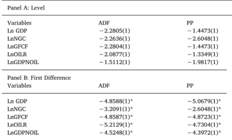
Tables 3 and 4renders the unit root test analysis. The need for the tests enhances accuracy of estimates and by extension avoid pitfall of misleading policy implication(s). Our study adopts the traditional unit root tests of ADF and PP. However, given the established criticism on the tests with size and power problem, we complement with Zivot-Andrews (ZA) unit root test that circumvents for these pitfalls men-tioned. All unit root tests are in harmony. That is, all the variables (that is, real GDP, NG consumption, real grossfixed capital formation, oil revenue and non-oil GDP) are integrated of order one I(1). Table 4 reports Zivot-Andrews unit root test that presents breaks. The estimated
break dates resonate with significant economic and political episodes of western sanctions and war periods in Iran. For example, the pre crises of global financial crises of 2006Q2 was captured. Also, the impact of sanctions imposed on Iran by most western nations, especially the US in the late 1980s is visible in natural gas variable and economic growth variable.
Table 5above reports the lag selection criterion. This is done to choose the most parsimonious and appropriate model. Our study adopts the Schwarz information criterion (SIC) for all subsequent analyses. The SIC is chosen over other available information criteria because of the large sample size and structure of our study.Table 6reports the coin-tegration relationship for all estimated models and affirms
Fig. 4. Visual plot of variables under consideration Source: Wold Bank (2018).
cointegration (long-run equilibrium) relationship. That is, there is a convergence between the real GDP, realfixed gross capita formation, oil revenue and non-oil GDP. This is established by the rejection of null hypothesis of no cointegration.Table 6used the real GDP and Non-oil GDP variables as dependent variable for the period under considera-tion. As a form of robustness check, we further carry out cointegration by ARDL bounds testing. The bounds test results presented inTable 7 corroborates the Bayer and Hanck results to confirm equilibrium re-lationship among investigated series while controlling for structural break dates in the estimation.
Having confirmed cointegration relationship among investigated variables, it becomes pertinent to investigate the long-run equilibrium coefficients. To achieve this, DOLS, FMOLS and CCR regressions are estimated to illustrate the magnitude of cointegration. The DOLS pos-sesses some unique traits that allow for estimation irrespective of the integration order of the variables. However, the explained variable is required to be integrated of order one. Also, the technique helps to ameliorate the issue of serial correlation and other internalities (Esteve and Requena, 2006).
The empirical results reflect a negative connection between income and oil rents; while natural gas rents and grossfixed formation present a positive connection with income in Iran between 1990 and 2017. The negative connection between oil rents and economic growth would be motivated by the existence of irregular behaviours (Arezki and Brückner, 2011) in Iranian economy system, as consequence of cor-ruption, development of political rights or civil liberties, which would reduce income levels in Iran (Ross, 1999;Arezki and Brückner, 2011). Thus, we consider that policymakers should be aware of the impact of oil rents over redistribution and corruption, in order to adopt measures
to attract the promotion of renewable technologies.
On the other hand, natural gas rents have contributed positively to enhance ascending economic growth in Iran (Mastorakis and Khoshnevis, 2014; BP, 2018). Pirlogea and Cicea (2012)found that natural gas consumption causes economic growth in Spain. The position of natural gas induced economic growth is also consistent to the study of Shahbaz et al. (2013c) found that natural gas consumption con-tributes economic growth in case of Pakistan. For the Iranian case, the country has been reflected as the second most massive natural gas field and the third producer of natural gas in the world as outlined by (EIA, 2018;BP, 2018). Iran was ranked the third largest natural gas producer in the world with more than 223 billion cubic meters of natural gas,
Table 2
Descriptive and correlation coefficients matrix estimate. Source: Authors' computation.
LGCF LGDP LNNGC LOILR LGDPNOIL Mean 7.0438 8.0535 3.1531 3.0562 14.1660 Median 7.1354 8.0758 3.1606 3.0973 14.2500 Maximum 8.0583 8.9661 3.5541 3.4856 16.3652 Minimum 5.6355 6.9852 2.5360 2.4372 11.4015 Std. Dev. 0.7116 0.6261 0.2806 0.2936 1.5240 Skewness −0.3243 −0.0815 −0.4585 −0.4963 −0.1775 Kurtosis 1.9009 1.5427 2.5794 2.6479 1.8396 Jarque-Bera 1.6966 2.2398 1.0601 1.1553 1.5339 Probability 0.4281 0.3263 0.5886 0.5612 0.4644 LGCF 1.0000 LGDP 0.9864 1.0000 LNGC 0.1413 0.0944 1.0000 LOILR 0.0473 0.1006 0.9766 1.0000 LGDPNOIL 0.9192 0.9331 0.0170 0.2173 1.0000
Fig. 5. Estimation Scheme
Note: Oil rents are not significant in both models.
Table 3
Unit root test results (without break).
Source: Authors' computation. Note:*. **, denotes 1% and 5% significance re-jection level respectively. Mackinnon (1996)one sided P-value is reported. Models with intercept and trend were reported for all test statistics. ( ) denotes optimal lag length.
Panel A: Level Variables ADF PP Ln GDP −2.2805(1) −1.4473(1) LnNGC −2.2636(1) −2.6048(1) LnGFCF −2.2804(1) −1.4473(1) LnOILR −2.0877(1) −1.3349(1) LnGDPNOIL −1.5112(1) −1.9817(1)
Panel B: First Difference
Variables ADF PP Ln GDP −4.8588(1)* −5.0679(1)* LnNGC −3.2091(1)* −2.6048(1)* LnGFCF −4.8587(1)* −4.8723(1)* LnOILR −5.2129(1)* −4.7304(1)* LnGDPNOIL −4.5248(1)* −4.3972(1)* Table 4
Zivot and Andrews unit root test results (with a single structural break date). Source: Authors' computation. Note:*. **, denotes 1% and 5% significance level of rejection respectively.Δ Denotes first difference and numbers in ( ) re-presents lag length.
Variables level Δ
ZA test-stat. Break Period ZA test-stat. Break Period
LnGDP −4.7194(1) 2006Q2 −5.7194(1)* * 2006Q2
LnNGC −3.5610(1) 2004Q2 −5.1224(1)* 2004Q2
LnGFCF −4.1319(1) 2000Q2 −5.1319(1)* 2006Q2
LnOILR −4.9720(1) 2004Q3 −5.7726(1)** 1999Q3
enjoying a 6.1-percent share in the global gas market (BP, 2018). The replacement of oil products with natural gas consumption was an es-sential policy of government in energy sector during the fourth devel-opment plan (2005–2009). Nowadays, more than 40% of total energy
consumption in Iran is provided by natural gas, reflecting the relevance of this energy factor in the process of economic growth and develop-ment plans (BP, 2018). We can as main reasons in the increasing rate of natural gas consumption is due to the low price of domestic supply of
Table 5
Lag criteria selection.
Lag LogL LR FPE AIC SC HQ
0 107.1262 NA 1.62E-06 −1.9832 −1.88149 −1.941992 1 760.7183 1244.339 7.65E-12 −14.2446 −13.7361 −14.03856 2 841.2461 147.1181 2.22E-12 −15.4855 −14.57014* −15.11466 3 849.749 14.88006 2.57E-12 −15.3413 −14.0191 −14.80567 4 855.0098 8.801689 3.18E-12 −15.1348 −13.4058 −14.43432 5 911.5698 90.27845 1.47E-12 −15.9148 −13.779 −15.04951 6 961.5902 75.99257* 7.78e-13* −16.56904* −14.0264 −15.53893* 7 968.0209 9.275018 9.56E-13 −16.385 −13.4355 −15.19008 8 972.8521 6.59645 1.22E-12 −16.1702 −12.8139 −14.81048
Note: where LR represent sequential modified LR statistic, FPE means Final prediction error. Also Akaike information criterion (AIC), Schwarz information criterion (SIC) andfinally Hannan Quinn information (HQ).
Table 6
Bayer and Hanck combined cointegration test results.
Source: Authors' computation. Note:*,**represents 1%, 5% significance rejection levels respectively Critical values for EG-JOH at 1% and 5% are 16.259 and 10.637 respectively, while for EG-JOH-BO-BDM are 31.169 and 20.486 respectively.
Models EG-JOH EG-JOH-BO-BDM Structural break cointegration remark
GDP = f(NGC,GCF,OR) 55.3399* 165.8640* 2006Q2 Yes
GDPNONOIL = f(NGC,GCF,OR) 56.8783* 115.8017* 2004Q2 Yes
Table 7
The ARDL test results.
Source: Authors' computation. Note:*,**represents 1%, 5% significance rejection levels respectively.
Cointegration by bounds testing Diagnostic test
Models Optimal length Break year F-statistics χ2white χ2ARCH χ2RESET
GDP = f(NGC,GCF,OR) 1,1,1,1 2006Q2 10.4592* 0.0876 0.3917 0.4010
GDP Non-oil = f(NGC,GCF,OR) 1,1,1,1 2004Q2 4.4768** 0.2805 0.1024 0.9167
Critical values
lower bounds 1(0) Upper bounds 1(1)
1% 3.65 4.66
5% 2.79 3.67
10% 2.37 3.20
Table 8
FMOLS, DOLS and CCR estimation results.
Source: Authors' computation. Note: *, **,*** represents 0.01, 0.05 and 0.10 rejection significant levels respectively. [ ] are t-statistics.
Depend variable: LGDP LNON-OILGDP
Variable FMOLS DOLS CCR FMOLS DOLS CCR
LNGC 1.327634*** 2.039091* 1.189030*** 15.22846* 11.80752* 11.53284* [1.682315] [4.834001] [1.577982] [7.998999] [6.855349] [6.690059] LOILR −0.153383 −0.034686 −0.166754 0.375406 0.088231 0.093588 [-0.908267] [-0.345241] [-1.046020] [0.921483] [0.215077] [0.253148] LGCF 1.717058* 1.844281* 1.676716* 6.302501* 5.601793* 5.502739* [11.34080] [24.50437] [12.38714] [17.25528] [18.22823] [17.60868] C −46.72872* −56.74880* −44.41514* −283.7136* −234.1770* −229.1904* [-4.690380] [-10.60986] [-4.813933] [-11.80470] [-10.72255] [-10.91274] R-squared 0.817568 0.889370 0.817089 0.870523 0.933854 0.898817 Adjusted R-squared 0.812453 0.875541 0.811961 0.866893 0.925586 0.895980 S.E. of regression 0.273145 0.223339 0.273504 0.635347 0.465999 0.561653 Long-run variance 0.225057 0.043931 0.225057 1.309762 0.732442 1.225689
Mean dependent var 7.983437 7.978626 7.983437 13.83643 13.84409 13.83643
S.D. dependent var 0.630724 0.633071 0.630724 1.741447 1.708275 1.741447
natural gas that leads to economic justification of the use of wasting energy technologies, non-optimal allocation, in appropriate and abun-dant use of natural gas. So, unlike the pattern of natural gas sumption in industrialized countries, the highest share of its con-sumption in Iran is allocated to the household and commercial sectors (Mastorakis and Khoshnevis, 2014).
During last years, sanctions has reduced gross capital formation in Iran, especially in construction investment and public investment (World Bank, 2017). From our piece of empirical results this variable presents a positive connection with income level, suggesting the ne-cessity of an advance in non-oil sectors, related with more sustainable growth. Hence, in medium-term the growth rates are expected to revert
to an average of 4% in Iran (World Bank, 2017), reflecting the positive effect that measures connected with sustainable growth would exert over this situation. So, our study suggests that the non-oil sector and private investments play a significant role, even oil sector lessens the enlargement of Iranian economy.
Our study further reveals that a 1% increase in NG consumption translates into a corresponding increase in economic growth by a magnitude of 1.3276%, 2.039091% and 1.1890% for FMOLS, DOLS and CCR respectively. Likely a 1% increase in NG consumption will amount into a corresponding increase in non-oil GDP by the following magni-tude 15.2284%, 11.8075% and 11.5328% for FMOLS, DOLS and CCR respectively.
Interestingly, our study observes positive synergy between real gross capital formation, economic growth and non-oil GDP. This is a call for Iran to strengthen her institutions in order to enhance capital accumulation both in the short and long-run and consequently grow her economy.
Thefitted model residual diagnostic tests results indicate that the model is adequate for policy construction given it free from auto-correlation, model miss specification and heteroscedasticity.
Fig. 2further buttresses the argument that thefitted model with real GDP as dependent variable inTable 8is stable, given the CUSUM and CUSUMSQ stability lines lie within the 5% threshold interval, an in-dication that the model is stable.
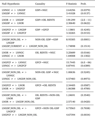
Table 9(Fig. 7) reports causalityflow of the variables under review (seeFig. 6). As shown, there exists a unidirectional causality running from gross capital formation to NG consumption. This implies that ca-pita formation is essential for increase NG consumption. Similar trend of unidirectional causalityflow is seen running from real GDP to gross capital formation. Our study gives support to a bidirectional causality between NG consumption and economic growth (Bildirici and Bakirtas, 2014;Solarin and Shahbaz, 2015;Ozturk and Al-Mulali, 2015;Dogan, 2015;Farhani et al., 2014;Saboori and Sulaiman, 2013;Balitskiy et al., 2016;Destek, 2016;Solarin and Ozturk, 2016;Esen and Oral, 2016; Hafeznia et al., 2017, among others-seeTable 1). This study joins the group of studies that support the NG-economic growth hypothesis (Lee and Chang, 2005;Reynolds and Kolodziej, 2008;Shahbaz et al., 2013c). However, NG driven economic growth is not a panacea for Iran's sus-tainable economic growth, given the dwindling price and energy market dynamics globally. This implies that there is need for diversi-fication of the energy portfolio in Iran to more environmental friendly sources like renewable energy sources is encouraged by this study (see Fig. 8) (seeTable 10).
The empirical results also support bidirectional causality between oil rents and economic growth in Iran, in line withNajjarzadeh and Mohsen (2004)andShahbazi (2013), who showed similar results for
Table 9
Pairwise Granger causality tests.
Null Hypothesis: Causality F-Statistic Prob.
LNNGC≠ > LNGDP GDP↔NGC 2.64256 (0.0379)
LNGDP≠ > LNNGC 3.41028 (0.0137)
LNOR≠ > LNGDP GDP↔OIL RENTS 139.299 (2.E−11)
LNGDP≠ > LNOR 2.30640 (0.0622) LNGFCF≠ > LNGDP GDP→GFCF 1.13801 (0.4245) LNGDP≠ > LNGFCF 3.32265 (0.0153) LNGDP_NON_OIL≠ > LNGDP NON-OIL GDP→GDP 8.93305 (0.0001) LNGDP_CURRENT≠ > LNGDP_NON_OIL 1.74898 (0.1514)
LNOR≠ > LNNGC OIL RENTS→NGC 3.25689 (0.0166)
LNNGC≠ > LNOR 1.84008 (0.1302) LNGFCF≠ > LNNGC GFCF→NGC 15.7445 (6.E−06) LNNGC≠ > LNGFCF 0.87441 (0.6389) LNGDP_NON_OIL≠ > LNNGC NON-OIL GDP≠NGC 1.00636 (0.5245) LNNGC≠ > LNGDP_NON_OIL 0.57483 (0.8973)
LNGFCF≠ > LNOR GFCF→OIL RENTS 2.34405 (0.0587)
LNOR≠ > LNGFCF 1.06388 (0.4789) LNGDP_NON_OIL≠ > LNOR OIL RENTS→NON-OIL GDP 1.24691 (0.3540) LNOR≠ > LNGDP_NON_OIL 2.57140 (0.0420) LNGDP_NON_OIL≠ > LNGFCF GFCF→NON OIL-GDP 0.73563 (0.7658) LNGFCF≠ > LNGDP_NON_OIL 4.67394 (0.0034)
Note≠ > means does not Granger cause.
Iran. The causality results validate the feedback hypothesis between energy and economic growth in Iran.
Finally, we apply Toda-Yamamoto causality test to reinforce em-pirical results.
5. Concluding remark/policy implications
This country-specific study seeks to investigate the interaction be-tween natural gas consumption-economic growth nexus for the case of Iran by the inclusion of real grossfixed capital formation and oil rents as additional variables in a multivariate framework in order to avoid omitted variable bias which previous studies failed to address. To do
this, quarterly data from 1990Q1 to 2017Q4 sourced from World Bank Development Indicators (https://data.worldbank.org/indicator) and the U.S Energy Information Administration database (EIA, 2018) was used for the econometric analyses. This study accounts for structural break in all estimations. For stationarity testing, beyond the conven-tional Augmented Dickey Fuller (ADF) and Phillips Perron tests, the Zivot Andrews unit root test that accounts for single structural break was also employed. For the cointegration analysis, with the noted break year properly accounted for in the estimation combined cointegration advanced by Bayer and Hanck (2013) is employed. The Bayer and Hanck (2013)test result was further confirmed via the Pesaran ARDL bounds testing to cointegration approach as a form of robustness test.
Fig. 7. Granger causality Scheme.
Fig. 8. VAR Granger causality Scheme.
Table 10
VAR Granger causality/block exogeneity Wald tests.
LNOR LNGDP LNGDP_NON_OIL LNGFCF LNNGC LNOR – 3.333597 4.209967 2.835539 7.708327 – (0.8525) (0.7553) (0.8998) (0.3590) LNGDP_CURRENT 22.96774* – 1.223886 10.63416 5.416463 (0.0017) – (0.9904) (0.1554) (0.6093) LNGDP_NON_OIL 13.96621** 17.07111* – 20.05350* 5.962063 (0.0518) (0.0169) – (0.0055) (0.5442) LNGFCF 5.270676 13.56803** 12.28014*** – 11.16886 (0.6270) (0.0594) (0.0917) – (0.1314) LNNGC 15.36548* 14.30384** 7.05745***9 7.743422 – (0.0316) (0.0460) (0.0917) (0.3558) – All 53.96707 37.03443 37.33722 59.21306 32.82844 (0.0023) (0.1181) 0.1116 (0.0005) (0.2421)