Electromagnetic radiation from multilayer printed
circuit boards: a 3D FDTD-based virtual emission
predictor
Gonca C¸ AKIR1, Mustafa C¸ AKIR1, Levent SEVG˙I2
1Electronics and Communication Engineering Department, Kocaeli University-TURKEY
e-mail: [email protected], [email protected]
2Electronics and Communication Engineering Department, Do˘gu¸s University,
Zeamet Sok. No 22, Kadık¨oy, ˙Istanbul TURKEY
e-mail: [email protected]
Abstract
A novel FDTD-based virtual electromagnetic compatibility tool for the prediction of electromagnetic emissions from a multilayer printed circuit board is introduced. Tests are performed with characteristic structures and sample simulation results are presented.
Key Words: Electromagnetic Compatibility, EMC, EM Emission, Printed Board, Microstrip Circuits.
1.
Introduction
Printed circuit boards (PCBs) and undesired electromagnetic (EM) emissions represent one of the most critical issues to be accounted for in electronic system design. The sizes are getting smaller and smaller and the speed higher and higher which results in severe EM compatibility (EMC) problems. EM fields radiated by high speed signal traces can cause both narrow and broad band interference to nearby electronic equipment, as well as leakage of data information. Generally speaking, undesired and unintentional EM emissions vary with the circuit structure and PCB layout [1, 2]. Source excitation is also a potential EMC problem [3, 4]. In order to avoid or reduce EMC problems, attention should be paid from the beginning, as early as the design stage. A number of efficient EMC approaches, such as layout, grounding, component choice, and positioning, etc., can be used. Also, system level solutions such as filtering, shielding, etc., are widely used [5, 6].
Modeling and computer simulation is one fundamental approach in EMC investigations of such PCBs. There are many EMC software and tools in the market. One well-known PCB design and EMC investigation tool is CST Microwave Studio [7]. Microwave Studio is based on integration technique. CST’s products cover an extremely wide range of EM components. Numerical simulation applications include static, stationary, low and high frequency problems. Typical applications include couplers, filters, planar structures, connectors, antennas,
inductors, capacitors, waveguides, etc. Another widely used package is the 3D Finite-Difference Time- Domain (FDTD) & Finite Element (FE) methods-based SEMCAD X [8]. SEMCAD X offers a simulation platform with accelerated processors for the investigation of a full range of typical EMC and Bio-EMC applications. Applications include mobile and stationary communication device compliance, medical systems analysis, implant safety, exposure setups, etc., [8]. FEKO is another method of moments (MoM) based tool being used extensively for EMC analyses [9]. The comprehensive implementation of the MoM, and hybridization with asymptotic high frequency techniques such as Physical Optics (PO), Geometrical Optics (GO), Uniform Theory of Diffraction (UTD), enable the analysis of electrically large problems. Other EMC tools are SI wave [10], FDTD-FEM [11]; EMC Studio, Transmission Line Method tool [12], and the XFDTD [13].
Here, a simple, easy-to-use, user-friendly virtual EMC tool, MGL-EMC, is introduced for the prediction of EM emissions from a multilayer PCB. The core of the MGL-EMC is based on 3D FDTD equations [14]. Perfectly matched layer (PML) termination is used in MGL-EMC tool [15]. The user only needs to render each horizontal layer of the PCB via picture editor. Also, basic dimensions and operational parameters such as the frequency band and simulation duration are user-supplied. Output data (signal vs. time) can be displayed on-line during the simulation. Once the FDTD simulation is over, results may be presented as emitted near field components vs. frequency, or emitted near field components vs. position, etc.
MGL-EMC tool is prepared using the FOX toolkit which is available under LPGL (Library GNU Public License). FOX is a C++ based Toolkit widely used in developing graphical user interfaces (GUI). It offers a wide and growing collection of Controls, and provides state of the art facilities such as drag and drop, selection, as well as OpenGL widgets for 3D graphical manipulation. (visit www.fox-toolkit.org for more details).
2.
The MGL-EMC virtual tool
MGL-EMC is a single executable file. A front panel appears once it is executed. At left, the problem space and PCB layout is produced via group of commands/buttons under Layout Controls block. Observation parameters are also in this block. Besides classical Windows commands like File, View , etc., at the top, menus to design and integrate PCB layers as well as animation commands are present. At the right of the front panel there are FDTD commands and buttons. Observation parameters are also selected from this block.
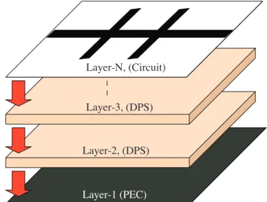
The introduction of the PCB is easy. The PCB is assumed to be made of horizontal layers. First one needs to draw each layer using any available design or picture software. PowerPoint software may also be used for this purpose. Most of well-known picture file formats such as bmp, gif, xpm, pcx, etc., are supported. Each horizontal layer is added from the Layer menu using the Load button (see Figure 1).
The thickness of each layer (i.e., picture file) is specified from the Layer menu under Layout Controls block (see Figure 2). The thickness of each layer is specified in terms of FDTD cell height Δz . Insert button is used for this purpose. The FDTD cell sizes are entered using the buttons under the Parameters menu at the right. The material properties of each layer are specified from the Materials menu under the Layout
Controls block.
Standard colors used in representing four different material types are: White for Material 0 (air), Black for Material 1 (perfectly electrical conductor, PEC), Orange for Material 2 (lossless dielectric with εr=2.4),
and Yellow for Material 3 (lossless dielectric with εr=2). Any other color and material type may be defined
re-entering new values. In order to use different colors for different materials a color margin should be used to eliminate possible errors that might be introduced from shades and color differences. This is controlled from the Layer ColorDef menu. In this case, for example, pictures drawn with different yellow tones are assumed to be the same material.
Layer-1 (PEC) Layer-2, (DPS)
Layer-3, (DPS) Layer-N, (Circuit)
Figure 1. Multilayer PCB design in MGL-EMC tool.
FDTD parameters, such as the size of the computation volume in terms of the number of cells along each axis, NX, NY and NZ, automatically appear under Parameters menu. The number of pixels of the picture file is directly set as NX and NY. The number of each pixel may also be set to different number of FDTD cells under the Material menu. By default, the number of time steps is set to 1500 and the number of PML cells to 8.
Two different excitations are possible via the MGL-EMC tool: a sinusoidal source and a Gaussian pulse. The Add button under Source Location helps to specify the source location. Source positions are colored white, the rest is black. The user may click on the white regions and locate a number of sources (see Figure 3a). The location of the added source appears inside x-pos and y-pos boxes near the Add button. The field component that is going to be recorded during the FDTD simulations is specified from Obs Layer menu (see Figure 3b). Once everything is set the scenario should be saved as “par.cme” which appears as the default scenario name on the screen. FDTD simulations start by clicking the Start button.
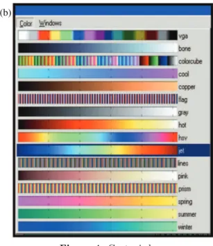
As shown in Figure 4, any component may be observed on the screen during the FDTD simulations. Animation colors may also be changed from the color palette (see Figure 4b).
Once the FDTD simulation is over, the Output Data file is automatically recorded with time-domain emissions (as amplitude vs. time of the selected field component). The EMC behaviors of the PCB in the frequency-domain may be obtained by using the Matlab code listed in Table 1.
Table 1. Off-line MatLab code for the FDTD data processor. % Program: MGL-EMC.m (Prepared by M. Çakır, May 2009)
% --- function GMEMC
close all; clc; clear ; N_sample=2048*2; nx=70; nz=90; VERI=load('Output_Data_Ht_s3.txt');
=VERI(:,2); dt=zaman(5)-zaman(4); fs=1/dt; freq=(0:(N_sample*0.01-1))*fs/N_sample; FREKANS=1e9; ii=1; for (i=1:3:nx)
jj=1 ; for (j=1:3:nz)
Xeks(ii,jj)=i; Yeks(ii,jj)=j; signal=VERI(:,2+((i-1)*nz+j)); BT=size(signal,1); for (t=BT:N_sample) signal(t)=0; end;
RF(ii,jj) =TtoF(signal',dt,FREKANS); jj=jj+1 ; end
ii=ii+1; end
figure; surf(Xeks,Yeks,RF ; title('DFT at 1e9 Hz'); BBBB=zeros(N_sample*0.01); for (i=1:5:nx)
for (j=1:5:nz)
Xeks(i,j)=i; Yeks(i,j)=j; signal=VERI(:,2+((i-1)*nz+j); BT=size(signal,1); for (t=BT:N_sample); signal(t)=0; end;
BB =fft(signal,N_sample); BBB=abs(BB)/(0.5*N_sample) for (i=1:N_sample*0.01); BBBB(i)=BBBB(i)+BBB(i); end; end
end
figure; plot(freq*1e-9,BBBB,'r'); grid on; function NORM=TtoF(signal,dt,freq); N=size(signal,2); k=freq*dt*N;
realW = 2*cos(2*pi*k/N); imagW = sin(2*pi*k/N); d1 = 0; d2 = 0; for (n=1:N)
y = signal(n) + realW*d1 - d2; d2 = d1; d1 = y; end
resultr = 0.5*realW*d1 - d2; resulti = imagW*d1; NORM=sqrt(resultr^2+resulti^2)/(0.5*N); % --- End of Code ---
iter =VERI(:,1) ; zaman
3.
Characteristic examples
Everything on the PCB layout directly affects EM emissions; the size, component types, trace lengths and locations, etc. The challenge to the EMC engineer is to minimize undesired EM emissions from the PCB without causing any degradation in its system performance. This necessitates a design procedure which takes into account all practical EMC rules from the beginning. The key in this design is the traces on the PCB. This is illustrated with the following example. Here, a microstrip line bandstop filter (BSF) is taken into account.
Three different filter structures having almost the same filter performances are designed and their undesired EM emissions are simulated and compared using MGL-EMC virtual tool.
Figure 3. (a) Source definition and (b) specification of field components to be stored.
Figure 4. Contunied.
Figure 5 shows the three microstrip line structures and their filter characteristics in terms of insertion loss vs. frequency. The center frequency of the filter is 1.5 GHz. All three filters are double armed with identical sizes; only arm shapes and positions are different, as shown in the figure.
0 -10 -30 -50 -40 -20 0.5 1 1.5 2 2.5 3 Frequency [GHz] Return/Insertion Loss [dB]
Scenario - 1 Scenario - 2 Scenario - 3
The lengths of the arms are L1 = 4 cm, L2 = 3.1 cm, the thickness of the dielectric substrate is 1 mm,
relative dielectric constant is εr = 2.4, input and output impedances are 50 Ω. A Gaussian pulse is used as
the excitation. The pulse’s significant frequency content extends from DC to 3 GHz. The FDTD computation volume is NX = 70, NY = 14, NZ = 90 with the cell sizes of Δ x = Δ y = Δ z = 1 mm. Emissions are recorded 4 cells above the PCB surface. Figure 6 shows total emissions vs. frequency for different field components. These figures are obtained via off-line FFT procedure applied on to the FDTD recorded simulation data.
As observed, although filter behaviors are almost the same, undesired emissions of these three microstrip line structures are quite different. For example, the emission in terms of x-component of the electric field of the third structure is almost four times higher than the other two at 700 MHz. Just the opposite is observed for the z-component of the electric field; emissions from the third structure are four times less than the other two. Emissions of the second structure seem to be the highest if y-component is taken into account.
Maximum and minimum emissions may also be observed as field distributions on horizontal layers above the PCB. In Figure 7, Ey distributions 4 cells above the microstrip surface at different frequencies, for the first
two filter structures, are shown. These figures show how arms of the filters resonate at these frequencies. The same is given in Figure 8 for the first scenario for the Ey distribution.
0.8 0.4 0 0.2 0.6 0 1 2 3 4 5 Frequency [GHz] Ex (f) 0.8 0.4 0 0.2 0.6 0 1 2 3 4 5 Frequency [GHz] Ey (f) 1.2 0.4 0 0.8 0 1 2 3 4 5 Frequency [GHz] Ez (f) 2 1 0 1.5 0 1 2 3 4 5 Frequency [GHz] Et (f) 2.5 0.5
z
z
x x
Figure 7. Ey distributions at different frequencies for Scenarios 1 and 2.
z z
x x
Figure 8. Maximum and minimum Ez emissions for Scenario 1.
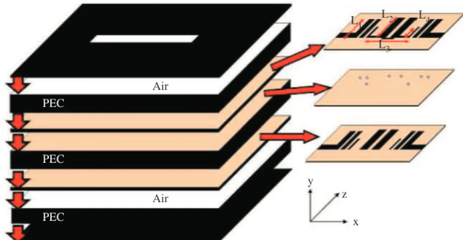
Another example is presented in order to show the strength of the MGL-EMC virtual tool. This is a multi-layer microstrip line circuit with and without a metallic enclosure having a rectangular aperture on the top. Layer-by-layer horizontal construction of this example is given in Figure 9. Here, a filter is constructed on a substrate with relative permittivity εr = 2.4 and thickness h=4 mm. Physical sizes of the filter are: L1 =
2.2 cm, L2= 2.7 cm, L3 = 2.8 cm, and L4 = 1.3 cm. The FDTD cell sizes are: Δx = Δy = Δz = 1 mm. This
NX = 84, NY = 14, NZ = 72 without the enclosure but increases to NX = 84, NY = 32, NZ = 72 with the enclosure (8-cell is reserved for the air-structure interface vertically). Also 8-cell PML is used to terminate the FDTD volume. Again, emissions in the time-domain are recorded 4 cells above the structure. Then, emissions as field components vs. frequency are obtained via off-line FFT procedure applied on to the FDTD recorded simulation data. Air Air PEC PEC PEC y z x L1 L2 L3 L4
Figure 9. Construction of the double-layer microstrip circuit and the enclosure.
Figure 10 shows total emissions vs. frequency without and with the enclosure for all three electric field components. As observed, emissions are dominant around 1.2 GHz, 2.0 GHz, and 3.5 GHz because of the antenna effects of the microstrip line arms L1, L2, L3, and L4. Also the pins between top and bottom
layers double the lengths of these arms. The enclosure with the rectangular aperture suppresses some of these dominant emissions, but magnifies many others.
Finally, Figure 11 presents the effects of the aperture of the PEC enclosure. The aperture on top of the enclosure is rotated 90◦ (i.e., the aperture is replaced with a cross-polarized aperture) and the simulation is run again. All other parameters are the same with the scenario shown in Figure 10. As expected, the locations of the horizontal aperture on top of the PEC enclosure do not affect the vertical field (Ey) components (vertical
emissions). On the other hand, horizontal emissions strongly affected by the polarization of the aperture.
4.
Conclusions
A novel numerical EMC analysis tool, MGL-EMC, is introduced for EMC investigations of PCB structures. MGL-EMC is based on FDTD method. Any microstrip line circuit can be designed in MGL-EMC, and time-and frequency-domain field emissions can be simulated. The user only needs to prepare picture files of each layer of the structure in various formats and import them one by one from the front panel. Visualization and video recording is also possible in MGL-EMC tool. The virtual tool can be used for both educational and research purposes.
0.2 0.1 0 0.4 0.2 0 0.3 0.1 0.12 0.08 0.04 0 0 1 2 3 4 5 Frequency [GHz] Ez (f) Ey (f) Ex (f) 0.8 0.2 0 0.4 0.2 0 0.08 0.04 0 0 1 2 3 4 5 Frequency [GHz] Ez (f) Ey (f) Ex (f) 0.4 0.6 0.12
Figure 10. Emissions as field strength vs. frequency with and without the enclosure.
Figure 11. Emissions as field strength vs. frequency with different apertures.
References
[1] H. W. Ott, “Digital circuit grounding and interconnection,” Proc IEEE International Symposium on Electromagnetic Compatibility, Boulder, pp.292-297, USA, 1981.
[2] R. Raul, et al., “A note on the optimum layout of electronic circuits to minimize electromagnetic field strength,” IEEE Transactions on Electromagnetic Compatibility, Vol. 30, No.1, pp.88-89, 1988.
[3] C. R. Paul, “Printed circuit board crosstalk,” IEEE International Symposium on Electromagnetic Compatibility, Wakefield, USA, 1985, p.75., pp.74-84, No. 1, 1988.
[4] T. Hubbing, et al., “Modeling the electromagnetic radiation from electrically small table-top products,” IEEE Transaction on Electromagnetic Compatibility, Vol. 31, No.1, pp.74-84, 1989.
[5] C. Paul, Introduction to electromagnetic compatibility, JohnWiley & Sons, Inc, 1992.
[6] M. I. Montrose, EMC and the printed circuit board; Design, theory, and layout made simple, J. Wiley & Sons Inc, 2007. [7] http://www.cst.com/Content/Products/MWS/Overview.aspx [8] http://www.semcad.com/simulation/ [9] http://www.feko.info/ [10] http://www.ansoft.com/products/si/siwave/ [11] http://www.efieldsolutions.com/ [12] http://www.emcos.com/html/emc studio.html [13] http://www.remcom.com/xf7#SlideFrame 1
[14] K. S. Yee, “Numerical solution of initial boundary value problems involving Maxwell equations in isotropic media,” IEEE Trans. Antennas and Propagat., Vol.14, pp. 302–307, 1966.
[15] J. P. Berenger, “A perfectly matched Layer for the absorption of electromagnetic waves,” J. Computat. Phys. Vol.114, pp.185–200, 1994.