A Comparison of the aggregation and disaggregation task allocation approaches in a random flexible manufacturing system

(1)

A COMPARISON OF THE AGGREGATION AND

DISAGGREGATION TASK ALLOCATION

APPROACHES IN A RANDOM FLEXIBLE

MANUFACTURING

^

A THESIS

SUBMITTED TO THE DEPARTMENT OF INDUSTRIAL

ENGINEERING

AND THE INSTITUTE OF ENGINEERING AND SCIENCES

OF BILKENT UNIVERSITY

IN PARTIAL FULFILLMENT OF THE REQUIREMENTS

FOR THE DEGREE OF

MASTER OF SCIENCE

fSSf-Maher lahmar

July 1997

(2)

A COMPARISON OF THE AGGREGATION AND

DISAGGREGATION TASK ALLOCATION

APPROACHES IN A RANDOM FLEXIBLE

MANUFACTURING SYSTEM

A THESIS

SUBMITTED TO THE DEPARTMENT OF INDUSTRIAL ENGINEERING AND THE INSTITUTE OF ENGINEERING AND SCIENCES

OF BILKENT UNIVERSITY

IN PARTIAL FULFILLMENT OF THE REQUIREMENTS FOR THE DEGREE OF

MASTER OF SCIENCE AAaKej- U Um a t

Bv

_Cv:-.· i/'

Maher lahmar

July 1997

(3)

11

I certify tliat I have read this thesis and that in my opinion it is fully adequate, in scope and in quality, as a thesis for the degree of Master of Science.

Assoc. Prof. Dr. Ihsan Sabuncuoğlu (Principal Advisor)

I certify that 1 have read this thesis and that in my opinion it is fully adequate, in scope and in quality, as a thesis for the degree of Master of Science.

Assoc. Prof. Dr. Cemal Dinçer

I certify that I have read this thesis and that in my opinion it is fully adequate, in scope and in quality, as a thesis for the degree of Master of Science.

Assoc. Prof. Erdal Erel

.Vpproved for the Institute of Engineering and Sciences:

(4)

T i

■I2i

-іаэ?·

(5)

ABSTRACT

A COMPARISON OF THE AGGREG ATION AND

DISAGGREGATION TASK ALLOCATION APPROACHES IN A

RAN D O M FLEXIBLE M ANUFACTURING SYSTEM

Maher lahmar

M.S. in Industrial Engineering

Supervisor: Assoc. Prof. Dr. Ihsan Sabuncuoglu

July 1997

The increased use of flexible manufacturing systems to efficiently provide customers with diversified products has created a significant set of operational challenges for managers. This technology is not only becoming more complex to control, but also presents a number of decision problems. Many issues concerning long-run utiliza tions and operational policies are still unresolved.

The primary objective of this study is to examine the effects of aggregation and disaggregation task allocation approaches of random flexible routings on the perfor mance of flexible manufacturing systems (FMS) and to analyze the effect of routing and sequencing flexibility on FMS and their interactions with other factors. The other experimental factors considered are machine load, alternative processing time ratio, local buffer capacities, set-up time, machine breakdown, processing time vari ation and scheduling rules. For this purpose, a simulation study is conducted and its results are analyzed by statistical methods.

Keywords : Flexible Manufacturing System, Aggregation and Disaggregation,

Routing Flexibility and Sequence Flexibility.

(6)

ÖZET

iş

GRUPLAMASI

v e

DAĞITILMASI YAKLAŞIM LARININ

RASSAL ESNEK ÜRETİM SİSTEMLERİNDE

KARIŞLAŞTIRILMASI

Maher lahmar

Endüstri Mühendisliği Bölümü Yüksek Lisans

Tez Yöneticisi: Doç. Dr. Ihsan Sabuncuoğlu

Temmuz 1997

Müşterilere çeşitli özelliklerde ürün sağlanmasına yol açtığı için kullanımı artan es nek üretim sistemleri yöneticiler için ise birtakım yeni sorunlar ortay çıkarmıştır. Esnek üretim sistemlerin hem kontrol edilmeleri karmaş

iktır, hem de yeni tip karar problemleri ortaya çıkarırlar. Uzun dönem kullanımı ve iş idaresi konularındaki bir çok sorun da henüz çözülmemiştir.

Bu çalışmada, iş gruplaması ve dağıtılmasının yaklaşımlarının esnek üretim sistem- leride rota ve sıralama esnekliği altında performansına etkileri incelenmiştir. Göze alman diğer deneysel faktörler de şunlardır: makina yüklemesi, alternatif üretim za manı oranı, lokal envanter kapasitesi, hazırlık süresi, makina buzulmaları ve üretim zamanı varyansı. Bu çalışmada bir berzetim çalışması yapılmış ve bu çalışmanın sonuçları istatistiksel metodlarla analiz edilmiştir.

Anahtar sözcükler: Esnek üretim Sistemleri, Iş gruplama ve Dağıtma, Rota ve Sıralama esnekliği.

(7)

VI

(8)

ACKNOWLEDGEMENT

I am indebted to Assoc. Prof. Ihsan Sabuncuoglu for his invaluable guidance, encouragement and the enthusiasm which he inspired on me during this study.

I am also indebted to Assoc. Prof. Dr. Cemal Dinger and Assoc. Prof. Erdal Erel for showing keen interest to the subject matter and accepting to read and review this thesis.

I can not fully express my gratitude and thanks to Burcu Gezgdr for her moral support and encouragement.

I would also like to thank Souheyl Touhami, Faker Zouaoui, Feryal Erhun and Tahar Ellejmi for their friendship and help during the preparartion of this thesis.

My special thanks to my parents in Tunisia who supported me during my studies in Bilkent.

(9)

List of Figures

3.1 Layout of the hypothetical F M S ... 9

6.1 Dispatching the jobs from central buffer to input queues ... 41

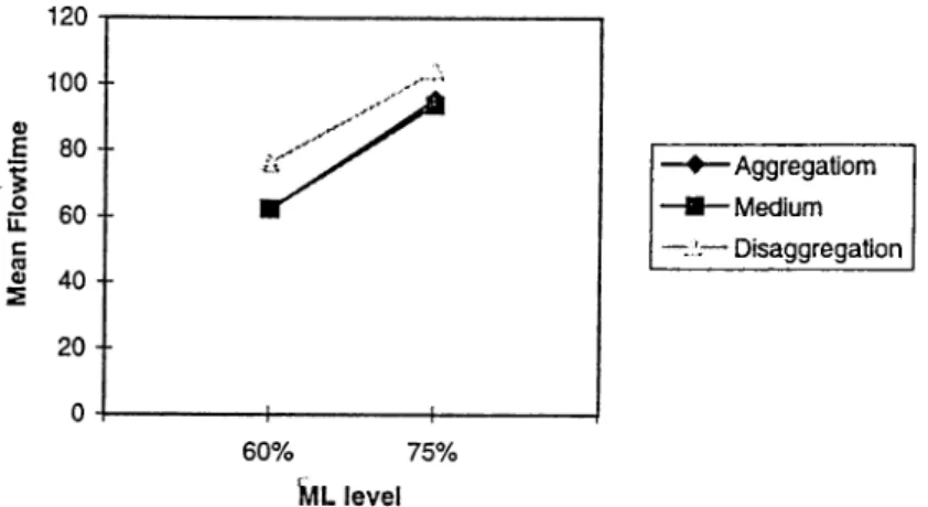
A .l Comparison of aggregation and disaggregation for varying ML levels using Model 1 ...52 A .2 Comparison of aggregation and disaggregation for varying ML levels

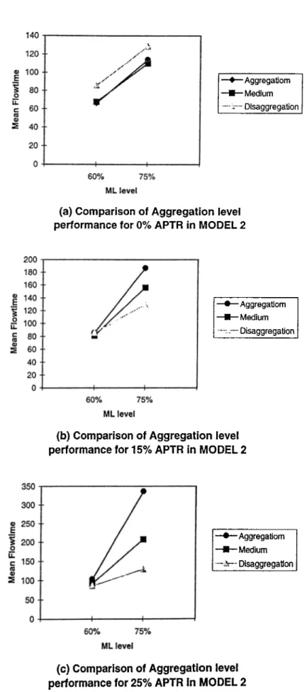
using Model 2 ...53 A.3 Comparison of aggregation and disaggregation for varying ML levels

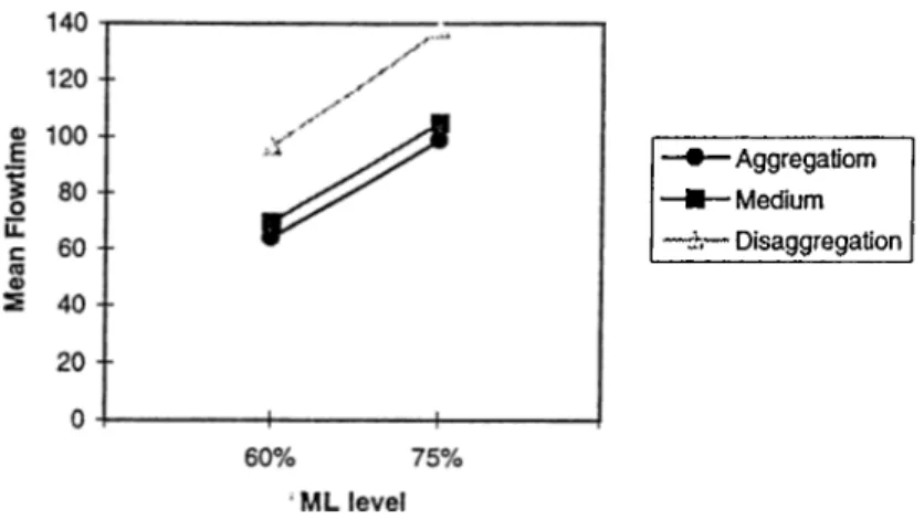
using Model 3 ... 54 A .4 Comparison of aggregation and disaggregation for varying ML levels

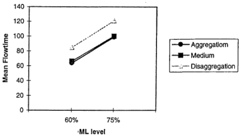
using Model 4 ... 55 A .5 Comparison of aggregation and disaggregation for varying A P T R lev

els using Model 1 ... 56 A .6 Comparison of aggregation and disaggregation for varying A P T R lev

els using Model 2 ...57 A .7 Comparison of aggregation and disaggregation for varying A P T R lev

els using Model 3 ...58 A .8 Comparison of aggregation and disaggregation for varying A P T R lev

els using Model 4 ... 59

(12)

LIST OF FIGURES

A .9 Comparison of flow-time vs. each factor level for each c a s e ... 60 A. 10 Comparison of flow-time vs. each factor level for each M o d e l ...61 A. 11 Comparison of aggregation and disaggregation for varying ML levels

using Model 1 under setup time co n s id e r a tio n ...62 A. 12 Comparison of aggregation and disaggregation for varying ML levels

using Model 4 under setup time co n s id e r a tio n ...65 A. 15 Comparison of aggregation and disaggregation for varying A P T R lev

els using Model 1 under setup time consideration ... 66 A. 16 Comparison of aggregation and disaggregation for varying A P T R lev

els using Model 4 under setup time consideration 69

A. 19 Comparison of flow-time vs. each factor level for each case under setup time con sid era tion ...70 A .20 Comparison of flow-time vs. each factor level for each Model under

setup time con sid era tion ...71 A .21 Interaction between setup time factor and other experimental factors 72 A .22 Comparison of aggregation and disaggregation for varying ML levels

using Model 1 under machine breakdown co n s id e ra tio n ...73 A .23 Comparison of aggregation and disaggregation for varying ML levels

(13)

LIST OF FIGURES XI

A .24 Comparison of aggregation and disaggregation for varying ML levels using Model 3 under machine breakdown co n s id e r a tio n ...75 A .25 Comparison of aggregation and disaggregation for varying ML levels

using Model 4 under machine breakdown co n s id e r a tio n ...76 A .26 Comparison of aggregation and disaggregation for varying A P T R lev

els using Model 1 under machine breakdown c o n s id e r a tio n ... 77 A .27 Comparison of aggregation and disaggregation for varying A P T R lev

els using Model 2 under machine breakdown c o n s id e r a tio n ... 78 A .28 Comparison of aggregation and disaggregation for varying A P T R lev

els using Model 3 under machine breakdown consideration 79

A .29 Comparison of aggregation and disaggregation for varying A P T R lev els using Model 4 under machine breakdown c o n s id e r a tio n ... 80 A .30 Comparison of flow-time vs. each factor level for each case under

machine breakdown con sideration ... 81 A .31 Comparison of flow-time vs. each factor level for each Model under

machine breakdown con sideration ... 82 A .32 Interaction between efficiency factor and other experimental factors . 83 A .33 Comparison of fiowtime under different factor levels for Normal and

Exponential distributions for Model 1 ... 84 A .34 Comparison of flowtime under different factor levels for Normal and

Exponential distributions for Model 4 ... 87 A .37 Comparison of flowtime for Normal and Exponential distributions

(14)

LIST OF FIGURES Xll

A .38 Comparison of flowtime for different CV levels under SF and RF 89

A .39 Comparison of flowtime for different CV levels under A P T R , Q and M L ... 90 A .40 Comparison of the interaction of scheduling rules with other factors . 91 A .41 Comparison of the interaction of scheduling rules with other factors

(15)

List of Tables

3.1 Experimental factor l e v e l s ... 13

B .l Detailed results for Model 1 94 B.2 Detailed results for Model 2 95 B.3 Detailed results for Model 3 96 B.4 Detailed results for Model 4 ... 97

B.5 Flow time results for the four Models 98 B.6 Difference between aggregation and disaggregation results 99 B.7 Flow time results of the three cases vs. ML for Model 1 and 2 . . . . 100

B.8 Flow time results of the three cases vs. ML for Model 3 and 4 . . . . 101

B.9 ANOVA results for the entire experimental d e s ig n ... 102

B.IO ANOVA results for the aggregation case ...103

B .ll ANOVA results for the medium aggregation c a s e ...104

B.12 ANOVA results for the disaggregation c a s e ... 105

B.13 ANOVA results for Model 1 and 2 106 B.14 ANOVA results for Model 3 and 4 ... 107

(16)

LIST OF TABLES XIV

B.15 Detailed results for Model 1 under set up time co n s id e ra tio n ... 108 B.16 Detailed results for Model 2 under set up time co n s id e ra tio n ... 109 B.17 Detailed results for Model 3 under set up time co n s id e ra tio n ...110 B.18 Detailed results for Model 4 under set up time co n s id e ra tio n ...I l l B.19 Flow time results of the three cases vs. ML for Model 1 and 2 under

set up time consideration...112 B.20 Flow time results of the three cases vs. ML for Model 3 and 4 under

set up time consideration...113 B.21 Difference between flow time performance without setup time and

under set up time consideration for Model 1 and Model 2 ... 114 B.22 Difference between flow time performance without setup time and

under set up time consideration for Model 3 and Model 4 ...115 B.23 ANOVA results for the entire experimental design including set up

time fa c to r ... 116 B.24 Detailed results for Model 1 under machine breakdown consideration 117 B.25 Detailed results for Model 2 under machine breakdown consideration 118 B.26 Detailed results for Model 3 under machine breakdown consideration 119 B.27 Detailed results for Model 4 under machine breakdown consideration 120 B.28 Flow time results of the three cases vs. ML for Model 1 and 2 under

machine breakdown con sideration ...121 B.29 Flow time results of the three cases vs. ML for Model 3 and 4 under

machine breakdown con sideration ...122 B.30 Difference between flow time performance without setup time and

(17)

B.31 Difference between flow time performance without setup time and under machine breakdown consideration for Model 3 and Model 4 . . 124 B.32 ANOVA results for the entire experimental design including efficiency

factor ...125 B.33 Detailed results for Model 1 under Normally distributed processiiig

t i m e ... 126 B.34 Detailed results for Model 2 under Normally distributed processing

t i m e ... 129 B.37 Flow time results of the three cases vs. ML for Model 1 and 2 under

Normally distributed processing t i m e ...130 B.38 Flow time results of the three cases vs. ML for Model 3 and 4 under

Normally distributed processing t i m e ...131 B.39 Difference between flow time performance under Exponentially and

Normally distributed processing time for Model 1 and Model 2 . . . . 132 B.40 Difference between flow time performance under Exponentially and

Normally distributed processing time for Model 3 and Model 4 . . . .133 B.41 ANOVA results for the flowtime under Exponential and Normal pro

cessing time distributions...1.34 B.42 Flow time results of the three cases vs. ML for Model 1 and 2 under

low CV le v e l... 135 B.43 Flow time results of the three cases vs. ML for Model 3 and 4 under

low CV le v e l... 136

(18)

LIST OF TABLES XVI

B.44 Difference between flow time performance under high and low CV

levels for Model 1 and Model 2 ...137

B.45 Difference between flow time performance under high and low CV levels for Model 3 and Model 4 ...138

B.46 Detailed results for Model 1 under LWKR scheduling ru le ... 139

B.50 Flow time results of the three cases vs. ML for Model 1 and 2 under LWKR scheduling r u l e ...143

B.51 Flow time results of the three cases vs. ML for Model 3 and 4 under LWKR scheduling r u l e ...144

B.52 Difference between flow time performance under LWKR and SPT scheduling r u l e ...145

B.53 Difference between flow time performance under LWKR and SPT scheduling rule ...146 B.54 ANOVA results for the flowtime under LWKR and SPT scheduling rulel47

(19)

Chapter 1 Introduction

A flexible manufacturing system (FMS) can be defined as a system composed of work stations mainly NC machines, automated material handling, and a computer controlled network that coordinates the activities of processing stations and mate rial handling system. These systems are highly automated and able to process a variety of part types simultaneously. The flexibility of an FMS is mainly due to the capability of performing several different types of operations within the same station and its material handling system which provides fast and flexible transfer of parts within the system. FMS came to fill the gap between high production volume transfer lines with low product variety and low production volume NC machines with high product variety. The major benefits of FMSs are higher machine utiliza tion, lower work-in-process, reduction in lead times, greater flexibility in production scheduling and higher labor productivity. However, a major drawback of FMSs is its high investment cost. Thus, many of the literature is attempting to study these systems to offer the industry with more efficient management ways to justify its cost.

FMS management requires the optimization of several problems that can be hier archically classified into design, planning, scheduling and control problems. Design problems deal with strategic decisions concerning the FMS hardware itself to meet the user goals and requirements. Specifically, the determination of the flexibilities and their levels, capacity of material handling system and buffers, number of pal lets and fixtures, type and number of CNCs are among these decisions. Planning

(20)

CHAPTER 1. INTRODUCTION

problems deal with tactical decisions concerning the part types for immediate and simultaneous production, allocation of machines to groups and tools to machines, task allocation of operations etc. The scheduling problem deals with detailed minute scheduling of machines, material handling system and other supporting equipments. Whereas, the control problem is concerned with monitoring the execution of the schedule and providing corrective actions in response to various changes in manu facturing environment.

Even though these decision problems are highly correlated, they are usually considered to be hierarchically related. In this study, we will focus on the process planning problem in an FMS. The objective of this study is to analyze the effect of task allocation on a flexible manufacturing system and particularly to compare the performance of the aggregation and the disaggregation process planning approaches in an FMS environment. The aggregation approach refers to the process of assigning all operations of a job to a single machine (or a single setup). The machine does not release the job until all required operations are processed on this machine. On the contrary, the disaggregation (or specialization) approach refers to the process of assigning operations of the job to various machines. The former approach is normally expected to reduce setup and transi^ortation times whereas the second aims to reduce capital investment in multi-purpose equipment and large tool magazines, facilitate the scheduling of jobs, and maximize the processing efficiency.

Probably, the only relevant study in this area is due to Kusiak [17] who stated that the tendency in process planning in automated systems is to assign as many operations to one setup as possible (i.e. aggregation). Since then no researches have questioned a validation of this approach in practice. However, we know that FMS can provide a wide variety of features that may not be always fully exploited by the practitioners such as flexibility. Flexibility refers to the ability of a manufacturing system to respond cost effectively and rapidly to changing production needs and requirements. This capability is becoming increasingly important to the design and operation of manufacturing systems, as these systems are called upon to operate in highly variable and unpredictable environments [13]. Thus, assigning all operations to a single setup may not be the most beneficial practice, but instead some operations can be processed on different machines due to routing and sequence flexibilities.

In the literature, most of the studies that deal with flexibility focus on the FMS scheduling aspect. Flexibility is not well investigated, specially in the literature of

(21)

CHAPTER 1. INTRODUCTION

process planning. One of the objectives of this study is to analyze the effect of sequencing and routing flexibilities and their interaction with other system design factors such as task allocation approaches, etc.

The remainder of the thesis will be devoted to this study and will be organized as follows: Chapter 2 contains a literature review that examines flexibility issues as it relates to our problem. This chapter is necessary to understand the different effects of flexibility on the performance of FMSs that have been studied in the literature. In chapter 3, we describe the hypothetical FM.S that we study, the model charac teristics as well as the experimental design and performance measures considered. Chapter 4 presents experimental results obtained by running the simulation based system under various conditions. ANOVA test is also conducted and its results are analyzed. In chapter 5, a sensitivity analysis is conducted by including set up times, machine breakdowns and considering different processing time distributions. In chapter 6, a discussion of the obtained results and explanation of the behavior of the system under the considered factors. Finally concluding remarks are made and future research directions are outlined in chapter 6.

(22)

Chapter 2 Literature Review

A flexible manufacturing system may exhibit total automation, or no automation at all and it can include fabrication as well as assembly. Stecke [11] defines five planning problems associated with flexible manufacturing systems, here we address the loading •problem^ which involves assigning operations to workstations (operation assignment) and routing jobs to workstations (job routing).

Stecke [11] proposes six objectives related to system utilization: to balance the assigned machine processing times, minimize movements between machines, balance the workload among machines. All the tool magazine as densely as possible and maximize operation priorities. Considering these objectives, she developed a 0-1 nonlinear integer programming model. She also proposes [33] a hierarchical approach to the loading problem based on a nonlinear formulation. Later, Berrada and Stecke [6] developed a branch and bound algorithm of Stecke’s model.

Kusiak [16] also formulates linear integer programming model considering tool life and workstation utilization constraints to minimize the total production cost and presents numerical examples.

Shanker and Srinivasulu [32] consider the throughput rate as the objective cri teria along with load balancing in their 0-1 integer programming model.

(23)

CHAPTER 2. LITERATURE REVIEW

Even though these studies provides good analytic formulations to solve the load ing problem, non of the above mentioned papers considers the routing flexibility available to the user after their model is solved.

Bretthauer and Ventaramanan [8] consider assigning operations to alternative machines without considering the tool life and machine capacity constraints.

Other authors focused on the minimization of the tool processing costs as an ob jective of their mathematical formulations to assure a better loading policy, whereas others included tool magazine constraints in their models.

Hence, most of the algorithms and models developed in the literature consider some of the above listed objectives assuming that it will assure a better perfor mance of the system. Such a decision seems to be ad hoc i.e. no analytical reasons for adopting one strategy over another exists and then can be only justified by large-scale simulation. In the literature some attempts to simulate task assignment models exist [15] and [20]. However, they are usually based on a special hypothetical manufacturing example that can not be generalized to other cases.

In our work, we will not consider these objectives but rather we will study the system performance under certain task allocation approaches. We will also inves tigate the effect of different experimental factors on the system performance. We believe that this step is necessary towards a general framework to understand the necessary operation aggregation levels for an efficient manufacturing.

In the second part of the literature review, we will focus mainly on the flexi bility issues as they are one of the important factors that are effecting the FMS performance under different aggregation levels.

Lin and Solberg [20] study flexibility issues for FMSs and provide interesting insights into how the managerial control system can influence the effectiveness of flexibility. They utilize both software and hardware flexibilities inherent in the system and conclude that it improves its performance. No improvement in the sys tem performance is noticed in breakdown case and deadlocks occurred frequently for some dispatching rules. No deadlock resolution scheme is implemented as it is the case in practice which deteriorates the system performance significantly. These results seem to be counter-intuitive and unrealistic since flexibility is expected to improve the system performance in the breakdown case whereas deadlock resolution

(24)

schemes are usually implemented in real situations.

Gupta and Guyal [14] examine the flexibility trade-offs associated with an FMS using simulation. The authors measure the impact of various types of flexibility on the system performance in an FMS under different loading, scheduling strategies and various system configuration. They note a trade-off among various flexibility types. These results show that the production output of a system can decrease as the overall flexibility of the system increases, and therefore the maximum production rate is not necessarily achieved at extreme flexibilities. Apart from their attempts, most of the literature isolate flexibility and investigate the effects of each flexibility alone regardless of their joint effects assuming that they are independent of each other [3], [4], [15], [21] and [23].

In other study, Benjaafar and Ramakrishnan [4] [5] note that flexibility is more valuable for highly loaded systems and that most of its benefits are realized with the initial introduction of a limited amount of flexibility (the phenomenon that they called as diminishing effect), therefore implementing a fully flexible system may not be always justified i.e. more cost will be incurred without getting significant benefits in return. The authors also noted that flexibility is more valuable for large systems and very effective in stabilizing it i.e. in maintaining a stable performance under changing conditions. They also observe that as the flexibility increases, the effect of scheduling rules looses its significance [3]. The same conclusion is also made by Mahmoodi et.al. [21] who considers AGV and machine breakdowns as a single factor of two levels. Such a practice may be misleading as both breakdowns have different and even opposing impacts on the system performance (i.e. machine breakdown may cause more waiting times in queues and favor disaggregation of operations, whereas AGV breakdown may cause higher utilization of the vehicles, more waiting time to be transported and therefore may favor aggregation of operations as it needs less materials handling). The authors also point out to the necessity of conducting research on the effect of partial routing flexibility on constrained FMS environments.

Similar conclusions are provided by Sabuncuoglu and Karabük [28]. The au thors note in their recent study that the highest level of improvement in the system performance is accomplished when a flexibility is introduced to the system for the first time (i.e, the system receives the most relief from flexibility when it is first applied). We also note that the positive impacts of the flexibilities on the system

(25)

performance are more significant when the capacities of the system resources are tight. Specifically, the effect of flexibility is greater at high machine load and low buffer size levels.

Barad [1] refers to flexibility as off-line and on-line versatility. Off-line is at the pre-release planning level and refers to load balancing and manufacturing feasibility options. On-line is made upon the occurrence of changes such as rerouting. The author concludes that the system performance increases under higher versatility and that versatility and control strategies are more effective at higher utilization levels.

In the literature, the alternative machines used for routing flexibility are assumed to be identical, (i.e, all of them can process the same operation in the same amount of time). In practice, however, alternative machines are usually less efficient than the ideal ones, causing longer operation times at routing flexibility.

To the best of our knowledge, most of the existing studies ignore the buffer capacities and assume the system to have infinite local and central buffer sizes. Others [20] suggest slack buffers that may keep a limited number of jobs in the system to avoid deadlocks. However, no study considered the local buffer sizes as an experimental factor. Also in the literature, the transportation times are not considered or assumed to be negligible or constant among different machines. In our study, we include material handling system since the transportation time may differ from aggregation to disaggregation models significantly. Moreover, the effect of such flexibility on aggregation and disaggregation is still a research issue.

In this study, based on a hypothetical flexible manufacturing system (Figure 3.1), we will develop a simulation model to compare the performance of aggregation and disaggregation approaches under various experimental conditions. Contrary to the current tendency in an FMS environment, we will study the behavior of the system under different aggregation levels and a variety of experimental conditions that are not yet well developed by the literature. We will also explore the effects of sequence and routing flexibilities on the system performance and their interactions with other factors, including task allocation approaches.

(26)

Chapter 3 Proposed study

In general the simulation model will use two sets of input data. System related data which consists of the physical description of manufacturing systems and values of environmental parameters which include the arrival rate of jobs, parameters of stochastic events, part types, machines and job flexibility, etc.

We first describe a hypothetical FMS that we use as a ’’ test-bed” for our ex perimental design. Then we define the parameters and conditions under which the system will operate. We present several assumptions that will be relaxed in a later stage. Then we define several experimental factors that we select to study their effects on the FMS. For this purpose, we will investigate the effects of machine load, alternative processing time ratio and buffer size on the system performance. A spe cial interest will be given to the interaction of routing and sequence flexibility with these factors and their effect on different aggregation approaches. We define four main models: The first model corresponds to the system without flexibility, the sec ond model uses sequence flexibility, the third model is based on routing flexibility and finally the fourth model combines both flexibilities.

We develop a simulation code for each model and run them under the differ ent combinations of factors. Then we compare the performance of different task allocation (aggregation) approaches and analyze the effects of flexibilities and their interactions with other factors. We also present some conclusions concerning the practical impact of our observations on the performance of FMSs.

(27)

CHAPTER 3. PROPOSED STUDY

<

-5

units

Figure 3.1: Layout of the hypothetical FMS

In this section, the FMS structure, model characteristics, descriptions of prob ability distributions, the experimental factors, experimental design, simulation lan guage and data collection procedures, and performance metrics used in this study are presented.

3.1 FMS Structure

The system is composed of seven stations. One station is the entering and exiting station that contains also a central buffer storage area of infinite capacity, whereas the others are regular machining centers. Each station has one multi-purpose ma chine, each with an input and output local buffer of finite capacity. Three identical AG Vs are used for materials handling in the system. The layout is composed of four squared areas, each side is of 5 distance units (Figure 3.1). The same FMS has been also used in the previous studies (Sabuncuoglu and Karabük [26]).

(28)

CHAPTER 3. PROPOSED STUDY 10

3.2 Model Characteristics

A widely recognized classification of FMSs characterizes as being dedicated or ran dom [10]. A dedicated FMS employs a set of general purpose machines, an auto mated material handling system, part specific pallet fixtures and magazines, with a fixed set of tools on each machine according to the predefined random sequence and route. It produces a small family of processing requirements. A random FMS employs a set of general purpose machines, an automated material handling system, modular pallet fixtures, and an automated tool loading system. It is capable of pro ducing a large family of widely differing parts. The product mix is not completely specified and the production schedule is subject to frequent changes.

The FMS to be studied in this thesis falls in the second category. To create such an FMS environment, jobs with random sequence of six different operations and random routing are considered. As tooling is an important issue which requires a separate and independent research, no tooling or pallet constraints are included in the model. Machines are allowed to process only one job at a time and the loading and unloading times are assumed to be negligible. No scrap or jobs to be reworked are considered. The machines and AG Vs are considered to be fully reliable. However, we relax this assumption later to see the impact of breakdown on the results.

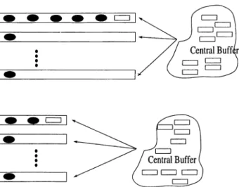
The jobs are generated randomly to the load/unload (L /U ) station and then dispatched to the machines. The jobs wait in a local input buffer when machine is processing another job. After completion of the operation, they wait in an output local buffer to be transported by an AGV. When the jobs visit all the assigned machines, they leave the system from this L/U station. After each transportation activity, the AG Vs park at the last visited station until a request is noted. The L/U station also serves as a central buffer with infinite capacity to avoid blockings and deadlocks of the system. There is always a possibility of blocking and deadlock if the buffer capacity is limited. A job may block a machine because it is not able to move on to another machine or consequent queue as that machine or queue is occupied by another job. This is known as blocking after service. In order to solve blockings and deadlocks, the job is redirected to the central buffer and waits until a vacant place is available in the input queues. At the flexibility models, the dedicated sequence and route may not be followed in which case, the machine route as well as the operation sequence is dispatched upon the system conditions at that decision

(29)

point of time. i.e. the job may be rerouted to another machine if the dedicated local input buffer is full etc..

3.3 Distributions

The arrival rate of the jobs to the system is based on a poison distribution with mean inter-arrival time of 10 through the simulation study. The job processing time is based on the exponential distribution with a varying mean according to the machine load. The means are determined through pilot runs to adjust the experimental factors at the desired levels. The exponential distribution is selected because it was also used in many simulation studies in the area ([3], [4], [25], [27]). The number of operations to be performed on each job is chosen to be six whereas the sequence of the operations was decided upon a discrete uniform distribution ranging from one to six. Each machine is visited only once.

3.4 Scheduling rules

It has been shown by Egbelu [12] that the most efficient scheduling rule to minimize the mean flow time performance of the system is SPT (Shortest Processing Time). This was later confirmed by Sabuncuoglu and Hommertzheim [27] who showed that scheduling the AGV system is as important as scheduling machines. The authors also note that the mean flow time is very sensitive to variation in the operation time distribution and increases with higher loads. In general, the scheduling rules perform similarly under low load situations, but at higher loads SPT is one of the best scheduling rules and STD (Shortest travel distance) is one of the best AGV scheduling rules under any other combinations. Thus in this study, the AGVs preference is ordered according to the STD rule and the jobs in local input queues are processed according to SPT rule. Because of the blockings and full input buffers, jobs are rerouted towards the central buffer. In order to minimize flow-time, these jobs are given the release priority.

(30)

3.5 Experimental Design

The experimental design is concerned with selecting a set of input variables to the simulation program, setting the levels of selected factors of the model and deciding on the conditions under which the model will be run. To examine the performance of each approach under different conditions, six experimental factors are considered: task allocation (TA ), machine load (ML), alternative processing time ratio (A P T R ), local buffer size (Q ), sequence flexibility (SF) and routing flexibility (RF).

Two levels of task allocation (TA) are considered: total aggregation of operations on the same machine or total disaggregation (specialization) of operations on all available machines. Each of these two aj^proaches is tested under various conditions. In later stage of our study, we introduce a medium aggregation level and compare it with these two extreme levels. Three levels of the machine load (ML) are considered, low, medium and high machine load levels (60%, 75% and 85% utilization). They are achieved by adjusting the mean of the processing distribution. Higher utilization levels may cause the system to be overloaded the fact that will be discussed later. The alternative processing ratio depends on whether the machines are identical or not. For the identical machines case, the operations are processed on any machine for the same amount of time. In the non-identical machines case, for each operation there is an ideal machine and other alternatives that can perform the operation in less efficient manner taking longer processing times. Thus the current alternative processing time ratio levels with respect to the ideal time are, 15% and 25%. In this thesis, this factor will be referred to as APTR.

The next factor, local buffer size (Q ), is simply altered by changing the local input and output queue capacities from 3 to 6 for low and high levels, respectively. Intuitively, flexibility is desirable in environments where machines are temporarily unavailable due to congestion, breakdowns, or blockings. The availability of al ternative operations and machines are generally expected to expedite the flow of parts through the system by reducing part waiting times and work-in-process lev els. Machine unavailability is more likely to occur in either highly loaded systems or in systems where demand, part processing requirements, or machine breakdown patterns are subject to variability.

In this study, we consider two types of flexibility, sequencing and routing. Se quence flexibility (SF) occurs when an operation can have more than one predecessor

(31)

Factor Low Medium High

Aggregation level Machine load (ML) Machine type (A P T R ) Buffer size (Q) Sequence flexibility (SF) Routing flexibility (RF) Disaggregation 60% ldentical(0%) 3 0 1 Medium 75% Non-identical(15%) Total 85% Non-identical(25%) 6 1 6 Table 3.1: Experimental factor levels

or successor. This sequence requires all operations to be performed and must incor porate all technological constraints, but allows choices in the order in which they are realized. It should be particularly valuable under the tight manufacturing con ditions. In the absence of a uniform framework for defining and evaluating sequence flexibility, many attempts are introduced to evaluate flexibility without achieving a definite measure of flexibility. In our model, we will rely on the measure proposed by Rachamadugu et al. [23]. Sequencing flexibility measure is either 1 or 0, 0 for null flexibility and 1 for total sequence flexibility, assuming that there are no se quencing constraints among the operations. This means that there are 6! feasible sequences. This also means that jobs have 6, 5, 4, 3, 2 and 1 feasible operations at their first, second, third, fourth, fifth and sixth production stages. Routing flexi bility measure is taken from Chang et al. [9] who define it in terms of the average number of machines that a particular operation can be processed at. It is assumed that the randomly dedicated machine is the ideal machine with the least operation time. Thus, (RF) is either 6 or 1, 1 for no alternative machine for the operations and 6 for total routing flexibility. This means that at each production stage we have 6 candidate machines to process the operation in hand. One will be the ideal one and 5 are alternatives. As alternative machines are less efficient than the ideal ones, they may require additional extra processing time that may take 3 values; 0%, 15% or 25% of the original processing time depending on machine type (Table 3.1). This experimented setup yields a 3^ x 2^ full factorial experiment.

In later stages of our study, we measure the sensitivity of the results to the addition of factors such as set up time, machine breakdown and different processing time distribution. Thus, we will deal with a 3^ x 2^ full factorial experiment.

(32)

3.6 Simulation Language and Data Collection

The models are coded in the discrete event simulation language SIMAN multi purpose simulation language [22]. The models are initially idle and empty, the AG Vs are located at the L/U station. Data collection starts when the system reaches a steady-state as determined by Welch’s procedure [19]. Common random numbers (CRN) is implemented to provide the same experimental condition across the runs for each factor combinations. This was done by dedicating independent random number generators to each source of randomness in the model. To insure the independence of the generated random numbers, different seeds are utilized through the simulation models. Due to the huge amount of computation time required for each run, data analysis is performed using five replications.

In this study, the method of batch means is used for simulation output data analysis. According to this method, a very long simulation run is broken down into smaller sub-runs. Our pilot experiments indicated that the warm-up period and batch sizes are approximately equal to 10000 and 2000 job completions. Since each completion run consists of five batches, we have the total run lengths for 10000 jobs. These simulation runs are repeated for each factor combination to implement the full factorial design. Because we manipulate random variability, a randomized complete block design will be used during the statistical analyses.

3.7 Performance Metrics

In this study, we are interested in the mean flow time of the jobs in the system. The average flow time of a job is broken down into eight components to facilitate the understanding of the systems behavior:

1. Average input queue flow time taken as the average time each job spends in the local input buffer of all machines visited.

2. Average output queue flow time taken as the time each job spends in the local output buffer of all machines visited.

3. Average processing time taken as the average time it takes to process a job on all visited machines excluding the blocking duration. It mainly differs according to

(33)

the machine load level.

4. Average set up time taken as the average time the job spends to be loaded or unloaded to the machine.

5. Average failure time taken as the average time the job spends waiting for the machine to be repaired. It is essential to note that breakdowns occur only when the machine is processing a certain part, thus it does not include the time the other jobs spend in a queue waiting for the machine to be fixed.

6. Average blocking time taken as the average time each job spends in a machine waiting for a vacant place in the output buffer after the job is processed, during this time, the machine can not process any other job and is just idle.

7. Average buffer queue flow time taken as the average time the job spends waiting in the central buffer for a vacant place in the input local buffer of the desired machine or for an AGV to be transported.

8. Average transportation time taken as the average total time during which the job is transported by an AGV through the different stations of the system. It mainly differs according to the grouping level of operations. In the disaggregation case, the materials handling takes place at least between 7 stations whereas it is just between 3 stations in the aggregation cases.

(34)

Chapter 4 Results

In this section, we present the results obtained by running the simulation models for the system described in the previous chapter. We differentiate four models. The first is the basic model where no flexibility is allowed. The second operates under sequence flexibility alone. The third one operates under routing flexibility alone whereas the last operates under both flexibility together. The results are analyzed res23ectively in this order.

4.1 Analysis of results

4.1.1 M odel 1 (Basic model)

The basic model is the simplest model where no flexibility is included. It can be viewed as a job shop with free-transported based materials handling. The sequence of machines to be visited is preassigned and each job has to follow the planned route and sequence through on. If the job can not find a vacant place in the input queue, it waits in the output or central buffer (depending on the actual location) until an available place is found. If the machine is blocked because of full output queue, a job is removed from the buffer and directed towards central buffer. The detailed

(35)

CHAPTER 4. RESULTS 17

results of Model 1 are given in Table B .l.

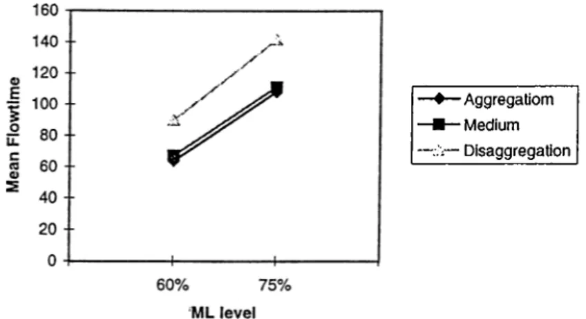
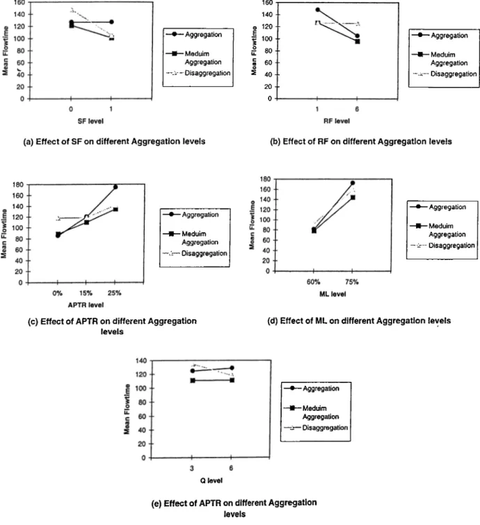
Our first observation is that in the identical inachines case, the aggregation approach performs better than disaggregation under all conditions (Figure A .l and A .5). This is due to the increase in waiting and materials handling times in the disaggregation approach which requires at least 7 moves between stations whereas aggregation requires only 2.

As the machine load increases, the flow-time increases under both approaches (Table B.5). However, deterioration in the system performance is more in the disag gregation case under low buffer size. Because at high system load levels, jobs have to wait longer in input buffers due to the higher processing times, which will also incur higher waiting times for jobs in output buffers, more reroutings and higher central buffer waiting times. This negative effect is higher for low buffer size as they offer less queue space for jobs. From such observations, we can safely conclude that aggregation is preferred in a system of identical machines. However, its performance deteriorates significantly with the increased machine load level.

For the non-identical machine case, again higher machine loads result in higher flow-times. However, contrary to the previous case, the deterioration of the flow time performance is greater for the aggregation case than the disaggregation case and this situation makes the disaggregation approach better than aggregation especially under high system toads. As seen in Table B.6 the difference between the aggregation and disaggregation increases for the favor of disaggregation as the levels of ML and A P T R increase. The reason for that is that total processing time under aggregation is somehow higher because of processing five operations out of six on alternative machines whereas the disaggregation assures that each operation is processed on the corresponding ideal machine. This means that the system is more loaded under aggregation approach.

It is interesting to note in the aggregation case that under the high ML and high A P T R levels, the system gets overloaded and therefore is unable to reach a steady- state. However, disaggregation case handles the situation without being overloaded as the jobs operations are dispatched to all the machines instead of only one.

For the basic model (Model 1), under all conditions, the large buffer capacity case performs better than the low size case. This is due to more capacity allocated to local buffers that reduce waiting times in central buffer and cause less reroutings.

(36)

In the aggregation case, no blockings are noticed because of the availability of AG Vs and an ample capacity of input buffers. However, in the disaggregation case, flow time increases with machine load. This is due to more jobs waiting in the previous output buffers. This certainly causes more blockings. Moreover, blocking times increase with lower buifer sizes as less capacity (i.e. less vacant places) becomes available.

4.1.2 Model 2 (Sequence flexibility model)

In the previous model we assumed that no interchange of operation sequence is allowed. In Model 2, this assumption is relaxed.

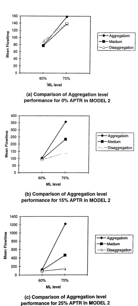
Sequence flexibility (SF) does not affect the aggregation case as the sequence of the operation of one job on the same machine does not change the performance of the system and hence the aggregation results for the basic model are still valid for Model 2. On the contrary, it positively affects the disaggregation approach due to more freedom of choice between the operations to be processed at a certain point of time according to the availability of machines rather than a single dedicated machine in the basic model. Therefore it allows higher machine utilization and shorter flowtimes. The detailed results of Model 2 are presented in Table B.2.

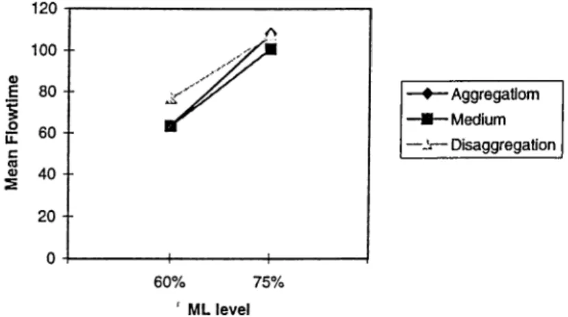
At the low load level for identical machines, SF improves the system performance slightly but aggregation is still better than disaggregation (Figure A .2 and A .6). At the high load, however, the disaggregation approach starts performing better. In fact, at the low load level, the jobs in the system have more available space to be allocated to and machines are less busy, however, at high load, less space is available and machines are busier. Thus, having flexibility at the low load level does not help much to improve the system performance, however it is more effective at the high load level. This fact is seen from the better performance of the disaggregation case at machine high loads.

For non-identical machines, disaggregation case is better for each A P T R level. The difference between these two task allocation policies increases as load and A PTR increases until the system gets more loaded (Table B.6). The superiority of disag gregation over aggregation is mainly due to the significant reduction in input buffer waiting time and central buffer waiting time. This decrease is a direct result of

(37)

flexibility that gives more freedom of operation sequencing, thus, not allowing jobs to wait as much as in Model 1 and hence reducing flow-time. In that regard, for non-identical machines case, the sequence flexibility becomes a crucial factor that works in favor of the disaggregation approach.

Again, under sequence flexibility, large buffer sizes improve the system perfor mance over the small buffers as the basic model case. This is due to more space avail ability for jobs in input queues which eventually reduces waiting time and reroutings to central buffer area.

To summarize, the sequence flexibility is not beneficial to the aggregation case and the same performance of the basic model is still recorded. However, in the disag gregation approach, the operations exchange sequence according to the availability of machines and buffer space and therefore improve the FMS performance.

4.1.3 M odel 3 (Routing flexibility model)

In Model 1 we assumed that the operation routings are pre-planned and fixed. We now relax this assumption and make the routing of the job operations subject to change according to the machine availability at that time without altering the operation sequence.

Contrary to sequence flexibility, routing flexibility (RF) provides benefits for both the aggregation and disaggregation approaches by allowing the processing of the operations on alternative machines rather than on ideal ones. Thus, the flow-time performance is expected to improve under both the aggregation and disaggregation approaches. The detailed results of Model 3 are presented in Table B.3.

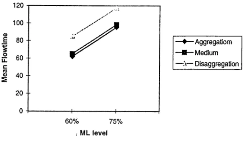
For identical machines, under both approaches the performance of the system improves, however, aggregation still performs better than disaggregation under all conditions (Table B.5). In fact, the improvement in the disaggregation case due to routing flexibility was not sufficient enough to make the performance better than aggregation (Table B.6).

(38)

CHAPTER 4. RESULTS 2 0

low load and A P T R conditions. However, at the high A P T R levels, the disaggrega tion performs better than aggregation and the difference between both approaches increases with the increase in ML and APTR. In fact, at the low load level, the need for dispatching to an alternative machine is too low due to available space in queues, however, as the system gets more loaded, less space is available and the jobs resort more and more to alternative machines making more use of the routing flexibility than at the low levels. This implies that as in the sequence flexibility case, routing flexibility is more effective at the highly loaded systems rather than lightly loaded ones.

An interesting result is that the low buffer size models outperforms the high buffer size models under all conditions (Figure A.3 and A .7). The only exception is noticed when the system is overloaded at very high ML and A P T R levels. This observation is difficult to interpret because of the interaction of multiple factors during simulation runs. But it is mainly due to the multi-channel versus single channel performance in queuing networks. In the next chapter, we will provide more detailed explanations about this observation.

The routing flexibility which is the main feature of Model 3 reduced significantly the flowtimes relative to Model 1. It enabled the system to overcome the congestion problems faced previously but didn’t give a clear advantage to one approach on the other.

To summarize, unlike the sequence flexibility, the routing flexibility improved the performance of both approaches. Its effect is greater at high system loads i.e. at high ML and A P T R levels. Moreover, the models with tow buffer size took more benefits from RF than larger ones.

4.1.4 M odel 4 (Routing and sequencing flexibility model)

In Model 4, both assumptions are relaxed. Hence, jobs can now resort to be pro cessed on alternative machines and operations among the same job can have different sequences according to the actual situation of the system. The detailed results of Model 4 are presented in Table B.4.

(39)

yields better results as compared to the models under each flexibility alone (Figure A .4 and A .8).

As the sequence flexibility just changes the order of the operations of one job, aggregation results in Model 4 are similar to those of Model 3.The low buffer size models still outperform the high buffer size models similar to Model 3. The same interpretations mentioned above are still valid for this model as well. For identical machines, the aggregation model outperforms disaggregation (Table B.6). For the non-identical machines, disaggregation performs better than aggregation and the difference between them increases with the high ML level and APTR. The aggrega tion case is overloaded at very high ML and A P T R levels. The previous explanations and suggestions still apply for this model.

As compared to Model 2 and 3, the flowtimes slightly improve (Table B.5). This is due to the contribution of both flexibility types. RF provides alternative machines whereas SF provides alternative sequences to process the operations of one job. Thus the effect of one flexibility in the presence of another won’t be as significant as in a single flexibility case. In other words, adding routing/sequence flexibility to sequence/routing flexibility will be beneficial only when the first introduced flexibility is unable to reroute the job to another machine/change its sequence.

4.1.5 Results of the medium aggregation level

In the previous section we have analyzed the behavior of the system under total aggregation and total disaggregation approaches for different experimental factors. However, real life systems may not operate under such extreme conditions. They may have so called a medium aggregation level. This level may differ from system to system according to its hardware characteristics, as well as the job requirements.

In this section, we consider a medium aggregation level such that the half of the operations of the job are assigned randomly to a machine whereas the other half is assigned to another one. In this case, the sequence flexibility will refer to the ability of exchanging the sequence of the two halves of operations of the same job; the possibility to process the second bunch before the first one. Routing flexibility will refer to the ability to process one bunch of operations on an alternative machine

(40)

instead of the ideal machine. The other factors are implemented in the model easily by altering some parameters values similarly to the previous cases.

The results of the experiments under this new setting are presented in Tables B.7 and B.8. In Model 1, the medium aggregation level performs better than the other extremes under high load and identical machines or under medium A P T R and low ML. But as the ML and A P T R increase, the disaggregation gets better than other approaches.

In Model 2, medium aggregation performs better than others under medium and low ML for identical machines and for low ML and medium A P T R level. Again when A P T R and ML increase, the disaggregation performs better than others.

In Model 3, even though the performance of the medium aggregation case is very close to the aggregation case especially at low and medium ML, it does not yield better performances than the other cases. In fact, this case is close to the aggregation case because for each job, two machine dispatching decisions have to be taken whereas it is only once for the aggregation case. This is not the case for disaggregation because six dispatching decisions have to be made.

In Model 4, the medium aggregation case shows better performance than the other cases under most factor combinations. The medium aggregation case per forms differently than the other cases because it is situated between aggregation and disaggregation. In other words, it makes use of routing and sequencing flex ibility more than aggregation but less than disaggregation does. The alternative processing time ratio contributes in increasing the flow-time in such a case more than disaggregation but less than in the aggregation case. The materials handling time is less than disaggregation but higher than aggregation. In that way, these factors interact at their different levels to make the medium aggregation case per form better or worser than the other cases. Similar to other cases, the medium aggregation case is overloaded under high A P T R levels, particularly under Models 1, 2 and 3 which is shown by the dark area in Tables B.7 and B.8.

(41)

4.2 A N O V A Results

The need for random number generation is indispensable in almost any simulation study. Therefore, the output of any simulation run is considered to be random. Thus, it is necessary to determine if the performance differences are statistically significant. We perform multiple comparisons between the mean flow-times (our considered criterion). For that purpose, we use the SAS package [31] to implement ANOVA F-test to indicate whether the means are significantly different from each other.

The analysis of variance (ANOVA) for the flow-time performance measure is given in Tables B.9, B.IO, B .ll, B.12, B.13 and B.14. In these tables, the source is considei’ed to be significant if it has a probability value smaller than 0.05 in the column named as ” Pr > F” . Blocking factor is also included in the ANOVA models to assess the effects of variance reduction (e.g. Common Random Numbers (CRN)) in the simulation experiment.

Since the system is overloaded at very high machine load (85%), some simulation runs under such high factor combinations especially at high A P T R levels do not represent a steady-state performance, the flow-time results are very large relative to the other found results. Thus, to avoid misleading ANOVA results, we decided not to include these runs in our statistical analysis.

As expected, ANOVA test for the entire results indicates that all the main factors and two-way interactions are significant whereas just those interacting with buffer size are not (Table B.9). As seen previously, TA, ML, A PTR, SF and RF showed to affect significantly the performance of the FMS.

As expected, the TA factor is significant. The performance of the system differ according to the task allocation approach. However, through our study, we inves tigate certain experimental conditions under which an approach may outperform another. The effect of TA on the system is quite complex. The complexity emerges from the different effects of the factor on different portions of the flowtime. For instance, the disaggregation causes higher transportation times whereas the aggre gation assures in general less central buffer waiting time. Another complexity comes from the interaction of this factor with the other factors. In the ANOVA result, the TA interacted with all the other factors except the buffer size. To analyze the

A Comparison of the aggregation and disaggregation task allocation approaches in a random flexible manufacturing system

A COMPARISON OF THE AGGREGATION AND

DISAGGREGATION TASK ALLOCATION

APPROACHES IN A RANDOM FLEXIBLE

MANUFACTURING

^

A THESIS

SUBMITTED TO THE DEPARTMENT OF INDUSTRIAL

ENGINEERING

AND THE INSTITUTE OF ENGINEERING AND SCIENCES

OF BILKENT UNIVERSITY

IN PARTIAL FULFILLMENT OF THE REQUIREMENTS

FOR THE DEGREE OF

MASTER OF SCIENCE

fSSf-Maher lahmar

July 1997

A COMPARISON OF THE AGGREGATION AND

DISAGGREGATION TASK ALLOCATION

APPROACHES IN A RANDOM FLEXIBLE

MANUFACTURING SYSTEM

Bv

Maher lahmar

July 1997

T i

■I2i

-іаэ?·

ABSTRACT

A COMPARISON OF THE AGGREG ATION AND

DISAGGREGATION TASK ALLOCATION APPROACHES IN A

RAN D O M FLEXIBLE M ANUFACTURING SYSTEM

Maher lahmar

M.S. in Industrial Engineering

Supervisor: Assoc. Prof. Dr. Ihsan Sabuncuoglu

July 1997

ÖZET

GRUPLAMASI

DAĞITILMASI YAKLAŞIM LARININ

RASSAL ESNEK ÜRETİM SİSTEMLERİNDE

KARIŞLAŞTIRILMASI

Maher lahmar

Endüstri Mühendisliği Bölümü Yüksek Lisans

Tez Yöneticisi: Doç. Dr. Ihsan Sabuncuoğlu

Temmuz 1997

ACKNOWLEDGEMENT

Contents

List of Figures

List of Tables

Chapter 1

Introduction

Chapter 2

Literature Review

Chapter 3

Proposed study

units

3.1

FMS Structure

3.2

Model Characteristics

3.3

Distributions

3.4

Scheduling rules

3.5

Experimental Design

3.6

Simulation Language and Data Collection

3.7

Performance Metrics

Chapter 4

Results

4.1

Analysis of results

4.1.1

M odel 1 (Basic model)

4.1.2

Model 2 (Sequence flexibility model)

4.1.3

M odel 3 (Routing flexibility model)

4.1.4

M odel 4 (Routing and sequencing flexibility model)