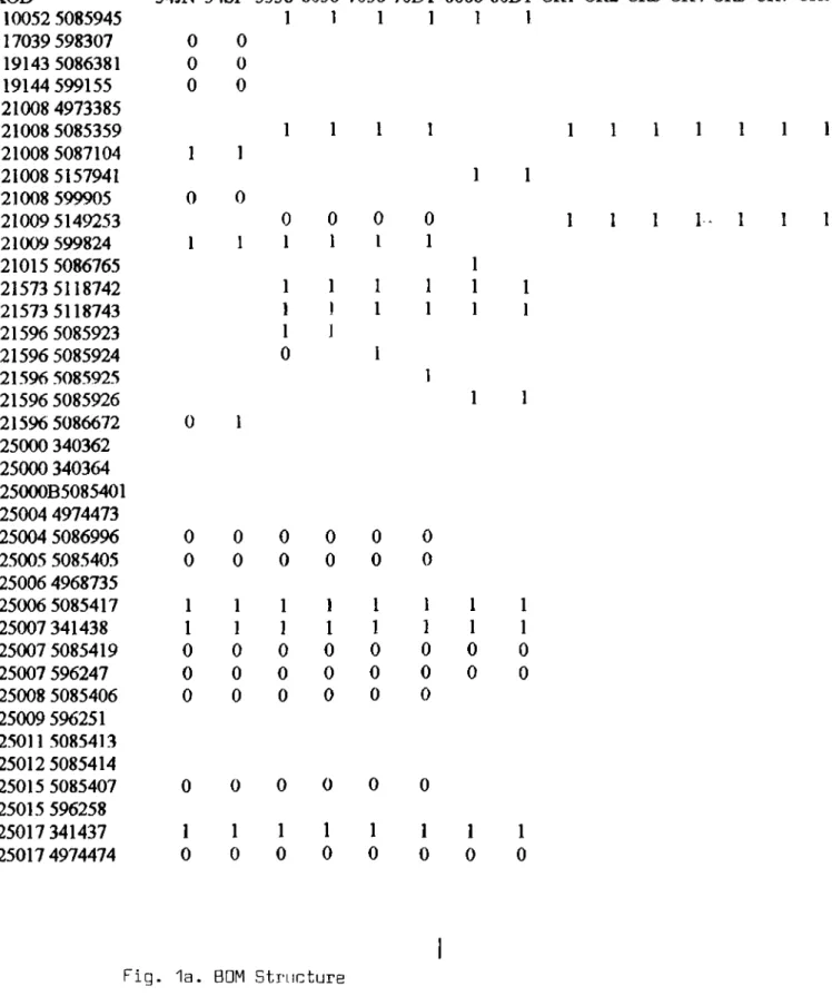
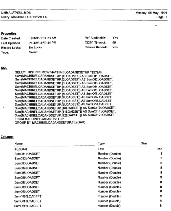
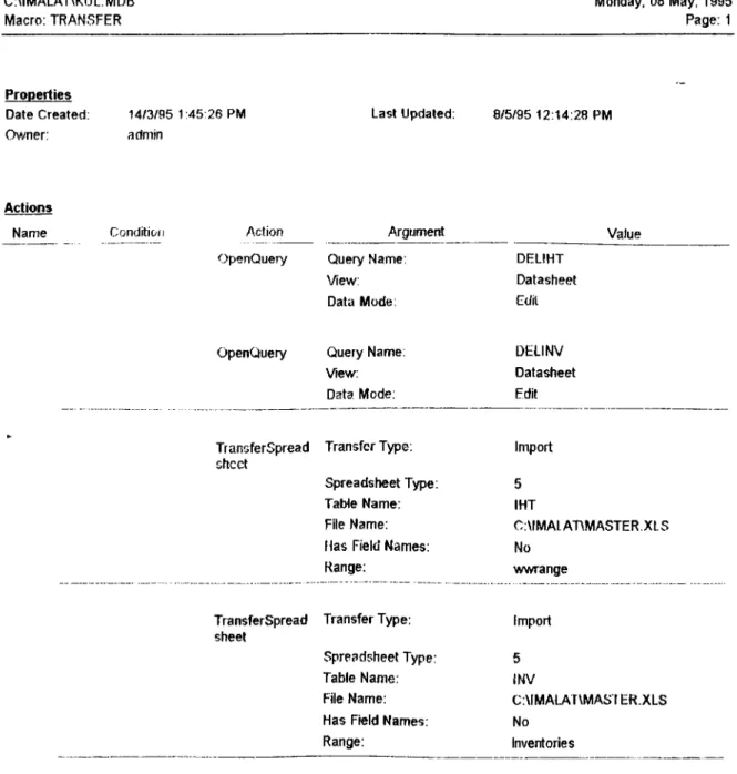
AN APPLICATION OF
SILVER MEAL HEURISTIC
TO MRP LOT SIZING DECISIONS
AT TÜRK TRAKTÖR FABRİKASI
A THESIS
SUBMITTED TO THE DEPARTMENT OF MANAGEMENT AND
GRADUATE SCHOOL OF BUSINESS ADMINISTRATION OF
BILKENT UNIVERSITY
IN PARTIAL FULFILLMENT OF THE REQUIREMENTS FOR THE DEGREE OF
MASTER OF BUSINESS ADMINISTRATION
I i и MO ■ L ^
I certify that I have read this thesis and in my opinion it is fully adequate, in scope and in quality, as a thesis for the degree of Master of Business Administration
Assoc.Prof Erdal Erel
I certify that I have read this thesis and in my opinion it is fully adequate, in scope and in quality, as a thesis for the degree of Master of Business Administration
Assist.Prof Murat MERCAN
I certify that I have read this thesis and in my opinion it is fully adequate, in scope and in quality, as a thesis for the degree of Master of Business Administration
Assist.Prof Serpil SAYIN
Approved for the Graduate School of Business Administration
ABSTRACT
AN APPLICATION OF SILVER-MEAL HEURISTIC TO MRP LOT SIZING DECISIONS
AT TÜRK TRAKTÖR FABRİKASI
By
Berkhan N. Esmer
Supervisor: Assist. Prof. Erdal Erel
MRP Lot-sizing, capacity planning, Silver-Meal, Türk Traktör Fabrikasi
MRP does not consider setup and inventory holding costs for lot sizing but very quick algorithms like Silver-Meal can be used for lot sizing decisions. A module to apply Silver-Meal Heuristic to manufacturing work order releases at Türk Traktör
Fabrikasy, Ankara, Turkey is designed and tested for 3 months. The module processes demand for finished goods, determines lot sizes, checks capacities by loading
machines according to the schedule and reports the setup, inventory holding and overtime costs. These cost figures are compared with the MRP lot sizes. It is observed that, the planning time decreased by 90% by designing module in PCs connected to the main databases, and the total costs decreased by 50%.
ÖZET
SILVER-MEAL METODUNUN TÜRK TRAKTÖR FABRİKASI MALZEME İHTİYAÇ PLANLAMASI KAFİLE MİKTARI BELİRLEMESİNDE
UYGULANMASI
Hazırlayan Berkhan N. Esmer
Tez yöneticisi: Assocc. Prof. Erdal Erel
Malzeme İhtiyaç Planlaması, kafile miktarları, kapasite planlaması, Türk Traktör Fabrikası
Malzeme İhtiyaç Planlaması, kafile miktarlannı hesaplarken tezgah hazırlama ve stokta tutma maliyetlerini göz önünde bulundurmazken, Silver-Meal Metodu bu amaç için kullanılabilir. Silver-Meal Metodunu kullanan bir modül geliştirilerek, Ankara’da bulunan Türk Traktör Fabrikası imalat atölyelerine iş emri verilmesinde uygulanmıştır. Bu modül bitmiş ürünlere gelen talebi alt parçalarma dağıtır, kafile miktarlarını belirler, makinalar üzerine gelen kapasite ihtiyaçlarını hesaplar, ve tezgah hazırlama, stokta tutma ve fazla mesai mahyetlerini raporlar. 3 aylık bir denemeden sonra, modülün ana sisteme bağlı bir PC üstünde geliştirilmesinden dolayı planlama zamanında %90, ve toplam maliyetlerde de %50 iyileştirme yaptığı saptanmıştır.
ACKNOWLEDGEMENTS
I gratefully acknowledge patient supervision and helpful comments of Assist. Prof. Erdal EREL, throughout the preparation of this study. I would also like to thank to other thesis committee members Assoc.Prof Murat MERCAN and Assoc.Prof Serpil SAYIN for their valuable comments and suggestions.
I also thank to my family and teachers for the opportunities, they give me, and special thanks to Gülay BİTİRİCİ for her kind support and patience.
TABLE OF CONTENTS
I. INTRODUCTION... 1
II. LITERATURE SURVEY... 4
III. TÜRK TRAKTÖR FABRYKASI... 7
III. 1. Company... 7
111.2. Organization... 8
111.3. Products and Production... 8
111.4. Production Planning Activities... 9
111.5. Review Of The Current System... 12
111.6. Performance Measures... 12
IV. DATA GATHERING... 14
IV. 1. Softwares Selected... 14
IV.2. Database... 14
IV.3. Bill Of M aterial... 15
IV.4. Operations, Direct Labor and Overhead... 15
IV. 5. Setup T im es... 16
V. DATA PROCESSING... 17
V . l. Setup C osts... 17
V.2. Inventory Holding C o st... 18
V.3. Overtime C osts... 19
V. 4. Scheduling Problem... 22
VI. THE MRP LOT - SIZING MODULE... 23
VI. 1. Purpose... 23
VI.2. General Framework... 23
VI.3. Master Plan Entrance... 24
TABLE OF CONTENTS
VI.4.2. Coding And The Results... 28
VI.5. Transfer Of D ata... 31
VI. 6. The Capacity Loading... 31
VII. THE APPLICATION OF THE MRP LOT - SIZING MODULE .. 34
VII. 1. The Master Production P lan ... 34
VII. 2. The Part Requirements And Lot Sizes... 35
VII. 3. Setup C osts... 36
VII.4 . Holding C osts... 38
VII.5. Overtime C o st... 41
VII. 6. Total C osts... 45
VIII. CONCLUSION... 48
VIII. 1. Database Usage... 48
VIII.2. Effects On Cost Figures... 49
VIII.3. Further Research Item s... 50 APPENDICES
CHAPTER I INTRODUCTION
Materials Requirement Planning (MRP) in production planning and control was first
used in 1950’s as the development in computer technology made it possible to process information at reasonable costs. After the product tree was configured, a master production
schedule and the records of inventory on hand were sufficient to form orders both for the
make parts and buy parts.
When the stable demands of the 1950’s left the ground to variable demands and
customized products with variations, traditional MRP applications did not answer to
production planning and control activities. The engineering change notices, and changes in
master production schedule were proved to be difficult to be handled in MRP systems.
Another drawback of MRP was the absence of the knowledge about the setup costs and
inventory holding costs to determine optimal lot sizes. To overcome this drawback, quick
procedures like Economic Order Quantity or Least Unit Cost, used to aggregate the orders in
different time buckets and by Silver-Meal heuristic, this lot-sizing decisions become very easy
to be solved.
With the improvements in technology, flexible manufacturing systems help the
production people to cope with variable demand and customized products with variations.
Just-in-time (JIT) philosophy, introduced by Japan manufacturers began to be analyzed by
Production Technique (OPT) and Single kanban systems are created. These systems required
low setup costs to produce many different products without making the lot sizes to increase
over demand for not to increase inventory holding cost and satisfy the need of the customer immediately.
The requirements of JIT philosophy caused JIT not to be applied very widely in US and
Europe. Zero lead time, zero inventory, zero set up times, zero defectives were not achieved by many manufacturers. For the products that they can accurately forecast, they shift to MRP-
like planning systems, and left the ones with changing demands to be handled with JIT and
some other production planning systems
For Turkey, situation is somewhat harder. The technological inefficiencies and
macroeconomics unstability caused manufacturers to build systems on personal experiences,
and production planning and control is made by persons rather than systems. For example,
Türk Otomobil Fabrikası (TOFAŞ) still has not constructed its product tree, Aselsan bought
Manufacturing Management (MANMAN) MRPII system in 1990, but used only Order Release
Module and could not install Capacity Planning Module. Turkish Aerospace Industry (TAI)
got the MRP system from General Dynamics, but they have the same problems of not loading
lead times and not using capacity planning modules.
In Turkey, although demand level is unsatiable, there are not so many customized
products, and for this reason the product trees, once configured, can be valid for years. This
One of the firms who use MRP and created a sophisticated product tree is Türk Traktör
Fabrikası in Ankara. In this study, lot sizing decisions of the dependent demand parts in this
firm will be made by an heuristic, which will consider inventory holding costs and setup costs and results of the heuristic will be compared with MRP.
In this sequel, literature survey on lot sizing decisions are presented in Chapter II.
Chapter III will give a general knowledge about the company. The data gathering for the study will be presented in Chapter IV. Data processing and assumptions will be stated in Chapter V.
The module generated to handle the lot sizing decisions and capacity planning will be described
in Chapter VI. The application of the module to the company’s planning process for the first three months of 1995 will be presented in Chapter VII. The findings from the study and further
CHAPTER II LITERATURE SURVEY
Lot sizing decisions on MRP systems have been studied by many researchers
considering setup and inventory holding costs. These researches have also identified capacity costs and tried to minimize total cost by linear programming models.
In their study, Olhager and Rapp(1985), used a linear programming model for
simultaneous lot sizing and capacity planning. The model used total cost to count for number
of setups required, and the average inventory level holding cost. The capacity problem is taken as a constraint and the interval of production is tried to be found by the interval which enables
the capacity of resources enough for production. The model requires the product tree to be
grouped as parents and off-springs. By the increases in number of parts, the model requires a
very accurate determination of the groups. The computational difficulty increases resulting
longer CPU time.
Tempelmeier and Helber (1994) also presented an LP formulation for the multi-item,
multi-level dynamic lot sizing problem under capacity constraints. Model tries to optimize the
set-up costs and inventory holding costs. The objective function is bounded by the capacity
constraint. The capacity constraints are taken into consideration as proportion of demanded
resource time to available capacity, and this ratio is bounded to be smaller than 1. As this ratio
requires the formulation of each product group to be spread over the families, and the number
of constraints increase tremendously by complex product trees.
The computational problems due to formulation is tried to be resolved by the heuristic
that is presented by the researchers. The heuristic takes the cost and demand as it reads the product tree. Then, the heuristic takes the first level in the product tree, and for each item in
that level determines the set of resources and allocate some manufacturing time in these
resources by the amount of demanded size. Then every resource is taken one by one and the allocated time for each item is summed. The lot sizing decisions are given by applying Dixon- Silver heuristic. Dixon-Silver heuristic tries to find the minimum cost per unit capacity by
looking forward the planning horizon. This heuristic is quite simple, but tries to minimize capacity costs in general. The comparisons are done according to the capacity constraints and
the inventory holding costs and setup times can deviate by 8-9% from the optimal solution.
Dillenberger (1994), proposed rather complex formulation to satisfy the requirements
of the real manufacturers on part types, machine groups, storable and non-storable resources,
setup families. Although these definitions were very helpful for the manufacturers, the
computational difficulties were hard to overcome. The computation time required for 44 types
of parts and 14 types of machines was 221.42 minutes and there were 3408 nodes to be
checked on IBM RS/6000-540 and AIX XL C/6000 VI. 1, known as the most sophisticated
hardware and software. So, thinking that the computation time will increase by the increased
number of parts and machines, LP formulation seems to be very inflexible and unsuitable for
real manufacturers who have over 500 parts and over 250 machines, even with this very
Computational difficulties also raise the interest to find out one time formulations like
EOQ to serve to balance inventory holding, and setup costs. Olhager and Rapp, on their trial to
improve the EOQ formulation which they blamed of not considering setup times as capacity
constraints, introduce capacity cost , queuing factor, processing times and furthermore they
pronounce the opportunity cost of capacity utilization. The total cost takes the costs of capacity, holding and setup cost. Capacity cost includes both used and excess capacity. Inventory holding cost occur both by lot sizing decisions and the increased queuing time by the
high capacity utilization of the machines. Here the formulation finds out first the extra capacity required and then the quantity that will be produced.
In literature survey, it was also interesting to find out that, the capacity and lot sizing decisions were transferred into spreadsheet designs, to increase the understanding of the people
and the usage by managers. Eppen, Martin and Schräge (1994), reported that Ford Motor Co.,
have designed scenarios and spreadsheets on Lotus 1-2-3. By the effective usage of these
spreadsheets by more people and managers. Ford Motor Co. post higher net income than
General Motors, which had followed an aggressive capacity planning strategy and faced with
too much capacity.
As a result of the literature survey, it can be noted that LP formulations have
computational and design problems when tried to be used in real life manufacturing firms
which have many parts to produce and assembly. And the improvements in Windows based
information systems are replacing mainframes and networks are becoming the future of the
computer science. The flexibility introduced by Windows and Oracle systems make it possible
CHAPTER
III. TURK TRAKTOR FABRİKASI
III.1. Company
Türk Traktör Fabrikası was founded in 1954 as Minneapolis-Moline Türk Traktör ve
Ziraat Makineleri A.Ş. The problems faced in Turkish market caused Minneapolis to leave the
factory to Italian Fiat, the State and Koç Group in 1959. In 1991, the State sold its shares to Koç Group and Fiat Agriculture is merged with New Holland Group. Recently, Koç Group has 75% and New Holland has 25% of share.
Türk Traktör Fabrikası is the oldest automotive plant in Turkey. In the first years, the
factory was more like an assembly line. Most of the parts were imported from the joint venture
Italian Fiat. By the industrialization of Turkey, TTF invested in different types of machines and
began to manufacture most of the parts internally. The developing suppliers began to supply
more parts for TTF. TTF still is a huge manufacturer with its 256 machines, 50 CNC’s, and
Heat Treatment Shop. There are about 2500 parts assembled, of which 500 is manufactured
internally including engine blocks, transmission, gearboxes, axles. There are about 4000
TTF has a functional organization structure. The three business functions, production, financing and procurement, are under the responsibility of three general manager deputies.
Production General Manager Deputy has engineering, production, quality control and
maintenance managers reporting to him. Procurement General Manager Deputy has the raw material procurement, part procurement, price analysis and sales departments supervising. Financial General Manager Deputy is responsible from finance, accounting, and cost
accounting managers. The Personal Department and Management Information Systems are
directly reporting to the General Manager. ( App .Al.)
TIT.3. Products And Production
n i.2 . Organization
Products of TTF are the tractors and crocieres(tractor bodies which are exported).
Tractors are varied according to their horse powers, gear boxes and tracks. Horse power is
varied from 55 HP to 80 HP, gear boxes from 8 front, 4 back to 12 front, 12 back and double
or single track are available. The products and their features can be seen in Table 1.
Table 1 Products of TTF
TRACTOR HORSE POWER GEARBOX TRACK
5 4 JUNIOR 55 8 SINGLE 54 SPECIAL 55 8/12 SINGLE 55-56 55 8/12 SINGLE 60-56 60 8/12 SINGLE 70-56 70 8/12 SINGLE/DOUBLE 80-66 80 12 SINGLE/DOUBLE CROCIERES “^^"■"»»^VVVVVVVWWVVVVVVVVVVVVVVWVVVVVV· 55-70 vvvvvwwvvvvvwvvwvvwwvwvvvvvvvvvwvvvwv8/12 VWVVVVW¥V¥V^r¥VVVVVVVVVVVWWVVVVVW^rtVV^íWVVVVVVVV^rı^>^SINGLE/DOUBLE
welding machines, and heat treatment machines of nitrurizing, sementation, inductions. The average age of the machines is 10-15 years. There are both very old machines and very new
ones like CNC’s which are flexible enough to be a part of CAM.
There are about 520 parts which are manufactured in the factory, from all of 2500 parts
assembled to the final product. The high labor cost, because of a strong union, force the firm to increase the proportion of buy parts. In turn, the factory managers want to manufacture high
value added parts like engine block and head, where the company invested $13 million, and crank shafts where $6.8 million will be invested. And small parts which requires less skillful
workers will be outsourced. By the increased number of high value added parts, the inventory
holding costs, set up costs and capacity costs are becoming more important to the company.
TTT.4. Production Planning Activities
The MRP logic is used for the production planning. There is a database which holds the
part usage quantities and the types that they are used in. There are 10 major types of tractor.
There are 12 other tractor types which are derived from these major categories, which change
in tire size, optional security frames, etc. which do not affect the manufacturing department,
because of these optional parts are all purchased from the side industries.
The lead times for the manufacturing parts are taken as one month for every part. Two
separate master production plans are prepared for manufacturing and assembly. The main
reason for two separate master plan is the capacity problem in the machining shop. The
months and used in peak demand months. Capacity is tried to be stabilized in this manner.
Also, production of spare parts are also scheduled in the first three months of the year. Capacity planning is made roughly considering only the one tractor’s capacity requirement in the machine shop multiplied by total production. The capacities of the resources used in the
machining department is not considered while preparing the master manufacturing plan.
Every month new production orders are given to the machine shop, just the amount
that are needed for that month’s manufacturing plan. No consideration of setup costs or inventory holding cost is made. No special properties of the parts are taken into consideration.
The capacity requirements on the resources is also left to the machining shop, and the problems seen are tried to be handled by overtime and more importantly by high stock levels.
The inventory turnover for the manufacturing parts is 5.8, which means there exists about two
months’ need of parts as WIP or ready-to-assembly.
The database used in TTF is quite rich and helping for the study. The accounting
system is not the standard but actual accounting system. This enables the cost of inventory
holding cost, and capacity cost known at each stage of production. The routes of the parts, the
standard machines for the operations, part usage, labor cost for each operation, standard times,
prices of the raw materials, overheads, book values of machines are all part of the database and
will be used in lot sizing decisions.
There are many schedule busters going on the manufacturing stages. Most common
one is the supply delays in raw materials. The delay seen in supply of raw materials makes the
breakdowns are seen frequently. Capacity problems are also tried to be solved by altering lot sizes, and lots are divided into smaller lots by machine shop.
Production Planning is made by a central planning department which is responsible from all orders and inventories for any part that is used in the finished goods or indirectly used
by the workers or in the production processes.
The procedure used in planning is simply MRP logic. A parts list has the parts and
quantities that are used in the products. The requirements for every part is calculated, then the available stock is subtracted, and the remaining quantity is ordered to the suppliers for buy
parts or material requirement forms are released to the Raw Material Warehouse, for the machining shop to manufacture the make parts.
The lead times are accepted to be one month for every make part, and these materials
releases are submitted to shop floor at the end of every month for the production of the
following month. The scheduling is handled by the Machine Shop Department. The operations
stocks are kept in the department by entering the Work Tickets which are filled by the direct workers who are reporting the time that they work and the quantity of the produced parts. By
the help of these operation stocks and the finished parts, shop floor schedules the production in
the machines by the most critical part that the stock level decreased to low levels. The main
aim of the shop floor is to make only one setup for every part for the whole load of one
month’s requirement. But, this principle sometimes broken, because of urgent parts that
require setup changes. Sometimes the lots of one month’s requirement is divided into smaller
nL5. Review Of The Current System
Current production planning activities result in high inventories, low throughput, and imbalance of material flow. The raw materials are transported to the machine shop on the last
week of the month and resources necessary for this activity are kept very busy on this week and idle on the other weeks. Again the initial operations for casting and forging materials are
heat treatment and some very common cutting and drilling operations. In the first week of the months overcapacity is faced on these machines. Because of the one month’s material flow to
the shop floor at the same time, the average inventory is about two weeks demand. If we add
one month phase difference between assembly and machining shops, this adds up to one month and a half months of inventory. When WIP is high, it becomes very hard to schedule jobs for
the machines. This mess sometimes caused manufacturing time to go beyond two months, just because of waiting in the queues for urgent parts to be processed.
TTT.fi Performance Measures
Since the goal is to minimize costs, the related costs with the lot sizing decisions must
be defined. The costs that are results of lot sizing decisions are inventory holding cost, setup
cost and overtime cost. As lot sizes are decreased, inventory holding cost is decreased since
average inventory levels decrease. Also, the queuing time can decrease leading to higher
throughputs. But, decreased lot sizes make it necessary to make more setups which can cause
capacity problems and increase setup cost. So, there is a trade off between inventory holding
cost and set up cost. At the same time, it is necessary to analyze overtime costs because
resources have finite capacities. A schedule must not load machines imbalanced that one week
captured by the overtime costs required by the resources to produce the work orders. The performance of the schedule, related to capacity, can be measured by total overtime cost.
For this study, inventory holding costs, setup costs and overtime costs will be
considered as the measures which can evaluate the performance of a manufacturing schedule
CHAPTER IV. DATA GATHERING
IV. 1. Software Selected
The software selected for this application is Microsoft Excel Ver. 5 and Microsoft Access Ver 2. The reason for making these applications independent from the mainframe is just
to have the advantages of the Era III* in Computer Technology. The networks enable the users
to access the company database by their personal computers and process the data to increase the effectiveness and flexibility of the users. To get benefit of the effectiveness and flexibility, MRP lot sizing problem is designed at PC by using PC software, but manipulating the data
from IBM A6 mainframe of Türk Traktör Fabrikası (TTF).
TV.2. Database
The firm has a big database that holds the parts list, the operations, the processing
times, setup times, machine overhead rates, the amount of material necessary, the stocks, the
stock movements, etc. The cost accounting system of the firm is actual costing, so that the
overhead values and direct labor costs are traced by the machines, and available data for the
holding costs can be obtained. The necessary data for a lot sizing application were available in
the factory. From these data, necessary tables to be used in Microsoft Access are created.
’ CASH, McFARLAN, McKENNEY,APLLEGATE, Corporate Information Systems, Texts and Cases. Era III is specified as the regulated free market in IT. The users are free to build their applications, but have to
IV.3. Bill Of Material (BOM^
The first important file for the MRP is the BOM. For the sake of the computational
simplicity, the tree structure is turned out into a matrix form, in which the dimensions are the
products produced and the parts used. The entries are the quantities that are used from that part in the given product. For the sake of matrix multiplication, the table is created in MS Excel Ver.5. as a spreadsheet. A portion of the sheet can be seen in Fig. la and the related
table in Fig. lb.
This spreadsheet is used to hold the part numbers, the required material for manufacturing, and the quantities used in tractor models. This table is necessary to obtain the
gross requirements of parts for the given planning horizon. The master production quantities
for every week in the planning horizon of 3 months will be entered in Microsoft Excel. By the
matrix multiplication of master production and PartsList, the requirement for every week will
be calculated in Microsoft Excel. Then the Silver-Meal algorithm, will formulate the necessary
lot sizes to be released to the shop floor every week, looking at the setup and inventory holding
costs.
IV.4. Operations. Direct Labor and Overhead
The routings for the parts that are manufactured in TTF are stored in TTF-A6 system.
These operations are used for the flow of material, the productivity measures, WIP counts,
The cost accounting system holds the labor costs and overheads for each operation and machine. When the table “operasyon” was created, the part number, operation number,
machine id, process time, direct labor cost, overhead rates are transformed into MS Access Ver.2. The table definition and fields can be seen in Fig.2. The fields in “Operasyon”, enables
to measure the base for inventory holding cost. The total value added in Machine Shop can be calculated from the operation table by the help of processing time, direct labor cost and
overhead rate. This table is mainly used for obtaining the base costs of parts to calculate the inventory holding costs, and to load capacities to the machines.
IV.5. Setup Times
Setup costs have never been calculated in TTF. Setup times are considered in the
scheduling process and it is thought that, setup is a cost element and when you increase the number of setups, you will have more costs and low efficiency. Set up times were stored in
Production Engineering files. The table Setup is created by transforming the partno, operation
CHAPTER V DATA PROCESSING
Performance measures selected to evaluate lot sizing decisions and schedules will be
generated by the processing of the data gathered from TTF A-6 database in MS Excel and MS Access.
V .l. Setup Costs
To find out setup costs of parts, the table “operasyon”, which hold partno, operation
no, machine id, direct labor cost, and overhead rate and the table setup is processed. The Query “setupcostsofop” is created. This query looks at the part routing from table “operasyon”
and for each operation of the part finds out the setup time necessary for the operation. For
every operation on the part, the required setup time is multiplied by the direct labor cost plus
overhead rate. The query can be seen in Fig. 4., with its properties, SQL, and fields.
The overhead is included in setup costs, because the only overhead cost that are not actually used during setup is electricity and coolants, which are a small portion in the
overheads. The other overhead items are forgone during setup, like engineering costs,
administration costs, etc.
After the setup time is quantified as a cost measure on every operation for a part, the
query “setupcostofparts” are created to sum up all the setup cost of operations of a part. The
Setup cost is considered to be a cost item in traditional cost accounting. But increased
necessity of flexibility in production looks at setup as a manufacturing time and only the inefficiencies in setup is considered as a cost. Modern accounting systems are supposed to look
at the time to manufacture the product from the order to the customer hands. And everything that will reduce this time will be considered as an asset. So in fact, frequent setups must be seen
as an asset, since it reduces the queuing time, decreasing WIP and increasing flexibility. But the capacity can be a constraint for frequent setups, if setup times are not less than an hour. But for
the machines that are not bottlenecks, or that have no capacity constraints, the setups are just a better usage of resources which will be idle because of low demand or which will be kept busy
to produce to stock.
V.2. Inventory Holding Cost
Inventories are unfortunately seen as an asset in balance sheets. But in fact, they are
huge amounts of money tied up in warehouses to bring 0% return. However, in Turkey, the
government bonds which have default risks, offer 10% of interest for a month.
For lot sizing module, inventory holding cost is considered to be 10% of the inventories
on hand for the month. The main reason for 10%, is the government bond rates. Although it is
obvious that higher interest rates are possible for a month, to measure the risks of tractor
manufacturing and compare with other alternatives that have the same risk level is beyond this
The holding cost for the parts consider only labor cost and overhead cost as the part base price. The raw material price is not considered as an inventory holding cost base. The only reason is that, the supplier contracts are designed to be shipments made between the 1st and 5th days of the months and shipments more than once in a month is not programmed in current A6 system. The shortest planning horizon is one month in all TTF-A6 database. Since,
there is no chance of regulating raw material shipments, the cost of raw material is not included in the base price of inventory holding cost.
The query “holding cost” can be seen in Fig.6. For every operation the total process
time is multiplied by the direct labor cost plus overhead rate. All the operation costs of the parts are then summed . The total cost can be seen as the total value added to the products in the machine shop. This total value add is the base for inventory holding cost. The WIPs and
finished products are multiplied by the base price and total inventory value is found. This total inventory level is multiplied by 10% for the monthly inventories and 2.5% for the weekly
inventories.
V.3. Overtime Costs
The capacity constraints are made roughly in most organizations. That is, the capacity
requirement for each finished product is known and this amount is multiplied by the production
quantities. This is very rough for many departments which have multiple resources to do the job. The problems of resources, temporary or permanent, can cause delays in previous jobs,
and most part of the available capacity can be allocated for these late one or two parts. Or the
most frequently faced problem, the late deliveries of raw materials from suppliers can cause a
But none of these problems can be detected by the rough capacity planning. These imbalances in production schedules in terms of capacity must be quantified to show the planner the result of the schedules and lot sizes on machine capacities.
In TTF, the workers are hourly paid and TTF is responsible to offer 9 hours of work
for five days of the week. So, whether the worker is idle during 9 hours of work or not is not
considered in wage pays. If the worker is in the factory, s/he will be paid. As long as the production schedules can cause many setups, but no overtime, there is no additional cost of the
lot sizing. But if the lot sizing cause overtime because of frequent setups, or very big lots, this may be an additional cost which will not be incurred if monthly releases were to be continued.
The idle time of resources caused by the new lot sizing procedure is not considered as a
cost, because every cost is a sunk cost. The price of the machine is paid, the salary of the worker will be paid, whether s/he will work or not. Overhead may be incurred during idle time
of the machine, but this will be double count of the overhead, because overhead cost is
included in trade off between inventory holding costs and setup costs, by including overhead
in the base price for holding cost.
Overtime cost will be found as the necessary overtime for the period, multiplied by the
direct labor cost plus overhead rate. The query “overtimecost” can be seen in Fig 7.a and 7.b.
with its properties, SQL and fields.
To calculate necessary overtime for the period, another query “machineload” is
designed. This query gives out the total time required for machines to process the parts which
query looks at the production schedule and lot size. For every lot to be processed, it goes through its routing and multiply the process time of operations by the lot size and stores the
result as the capacity load for the machine.
The setup times necessary for the machines are added to the process times by the query “machineloadandsetup”. This query looks at the production schedule over the planning horizon and adds setup times for parts that has been scheduled to be manufactured. This query can be seen in Fig. 9. These costs are aggregated to weekly costs by the query “machineloadbyweek”
in Fig. 10.
By the aggregation of necessary processing and setup times for machines, the required
overtime can be calculated by the difference between capacity loads and current capacity of the
machines.
Although the capacities of machines for the planning horizon must be stored as a table
to decide about overtime, there were no available data on this issue. Machine shop was working two shifts, and they were trying to use all the machines for two shifts. So, the capacity
of every machine is taken as 5*16*60 = 4800 minutes per week. If the breakdown rate data
TTF has no available data on lead times. The one month inventory of the
manufactured parts is sufficient for every part and used as a lead time. But as the CNCs are increasing in machine shops, one week of lead time becomes a reality.
The lead time for any part will be one week. So, the lead time is taken as a week for every part, and forward scheduling is made to anticipate the loads on the machines. It is
assumed that if the work order of a part is released to the shop floor, it will be manufactured within that week. This fact simplified the scheduling problem, and no consideration of
backward or forward scheduling is made.
CHAPTER VI
THE MRP LOT - SIZING MODULE
VI. 1. Purpose
The purpose of the application module is to present the users a flexible, helping and friendly alternative to lot sizing decisions of work orders by the use of Silver-Meal Heuristic.
The application module must be easy to understand and utilize, and must be accurate and
reliable. Also, the module must show the situation from different perspectives like setups,
inventories and capacities.
VT.2. General Framework
The general framework of the MRP Lot Sizing Module can be seen in App A2.
Application module starts with the master plan entrance. These amounts are multiplied by the
usage quantities of the parts and gross requirements are obtained. These requirements are
processed by Silver-Meal Heuristic and the lot sizes and schedules are processed by several
queries to obtain the machine loads, setup costs, overtime costs. The decision maker can go
through these queries and fine tune the schedules.
First option is the production plan entry. Master Production Plan can be entered to the
system by this option. The other option under Data Entry is the transfer of data. The data on
option is selected. The other option group is Details of Part Schedules and Machine Capacities. Capacity load of a machine, or the route of a part that will go through can be seen with these
options. The option group of Cost By Parts and Machines, gives out the setup costs and inventory holding costs of selected parts and overtime costs of selected machine. Costs by
Weeks option determine the total setup, inventory and overtime costs by periods in the
planning horizon.
VL3. Master Plan Entrance
Master Plan Schedules are prepared by the Production Planning Department.
Production Planning Department determines the assembly schedules of the tractors and prepares a Manufacturing Master Plan accordingly. The amounts of tractors that must be
manufactured by the machine shop is converted into work orders on parts and delivered to
Machine Shop.
A sample production plan can be seen in Fig. 11. The products to be manufactured, the
production amounts and the production weeks are determined in the schedule. Master Plan
Entrance is designed in MS Excel. The main reason is to utilize the MS Excel matrix
multiplication functions and MS Excel Visual Basic Programming Language for the data to be
processed by Silver-Meal Heuristic. By the entrance of Master Plan, MS Excel multiplies the
production amounts, by the part usage quantities and drives out total requirements for each
part. The result of these matrix multiplication is put in a spreadsheet to be processed by Silver
A sample portion of these sheet can be seen in Fig. 12. In this portion, setup costs and
holding cost for the parts which were calculated in queries of MS Access is copied. Silver-Meal Algorithm will use this data after, when lot sizing decisions are to be made.
VI.4. Silver And Meal Algorithm
Lot-Sizing heuristics were tried to be made by Linear Programming models in order to
have an optimum solution. But the necessity of a high computational power to process complex production facilities, some heuristics were created, like Economic Order Quantity.
Silver and Meal in 1973 developed the heuristic which try to minimize the total relevant
costs per unit time for the duration of the planning horizon. The heuristic was intended to cover the drawbacks of Economic Order Quantity which requires very stable demand patterns
and Wagner - Whitin approach which have complex nature of algorithm, and require a well-
defined ending point for the demand pattern, and the necessary assumption that replenishments
can be made only at discrete intervals.
If a replenishment arrives at the beginning of the first period and it covers requirements
through the end of the Tth period, then the criterion function can be written as :
(Setup Cost") + (Total Carrying Costs to the End of Period T1 T
V L 4 .1 The Essence Of Algorithm
The replenishments at the beginning of the periods force the planners to make
replenishment quantities that last for an integer number of periods. Consequently, it can be thought that, decision variable for a particular replenishment will be T periods that the
replenishment will last, with T constrained to integer values. The replenishment quantity Q, associated with a particular value of T is ;
Q = S Demand(j) j=i
According to the chosen criterion, decision variable is the number of periods T, which
will minimize the total relevant costs per unit time of replenishment and carrying costs over the
time period T.
If total relevant costs associated with a replenishment that lasts for T periods, denoted
by TRC(T), then we can use TRCUT(T) to denote the cost per unit time, where :
TRCUT - TRC(T) / T = ( Setup Cost + Inventory Holding C ost) / T
The basic idea of the heuristic is to evaluate TRCUT(T) for increasing values of T until,
for the first time ,
that is the total relevant costs per unit time start increasing. When this happens, the associated T is selected as the number of periods that the replenishment should cover. The
VI.4. 2 Codin2 and the Results
Silver Meal heuristic is coded on Microsoft Excel Ver.5 by Visual Basic. The spreadsheet holds the requirements for each week for each part and the setup and holding
costs.
The procedure first finds out TRCUT(T)s for every period and writes on the spreadsheet. When the TRCUT(T+1) > (TRCUT(T), the total amount of requirements
necessary for T periods is taken as a release for machine shop and again written to a separate region of the spreadsheet.
The code of the algorithm can be seen in App. B3. The algorithm starts with initializing
the old values. Then it gets critical data of the planning horizon, number of items that will be planned, and the interest rate that will be valid for the planning horizon. Although it is possible
to include forecasted interest rates that will be valid for each period, in Turkey it is very hard to
see the coming periods valid interest rates. So, one interest rate is made relevant to all periods
in the planning horizon.
Then the loop that will take the parts one by one is started. The loop runs for the
number of parts that is defined in the constant parameter of t j3arts(total number of parts).
When one part is started to be executed by the algorithm, released quantity and last released
period values are initialized to 0 and 1 respectively. That means that, there have been no
released part lot to be manufactured, and the last period that the lot release was given is the
These two variables are the backbones of the algorithm. First parameter, released actually holds the lot size that will be released to the manufacturing departments. This is the
decision variable Q which is the sum of demands of the periods which are to be satisfied with a
single production lot. The other parameter lastrel holds the last period that the demand was satisfied. So, when the lot size decision made for the succeeding production, the period that the
lot will be released is the lastrel period, because this periods demand is not satisfied yet.
After these initializations, algorithm starts and began to calculate period costs. The
period cost TRC(T), is simply the setup cost plus inventory holding cost. Setup cost is taken from the second column of the requirements sheet which can be seen in Fig. 12. The inventory
holding cost is somehow harder. The inventories to be hold differ in number of periods that is stocked at shop floor or warehouses. When you give a lot that will be enough to satisfy
demands of 100,150,200 parts per period, first period demand is not stocked. It is pulled in the first week. But 150 of them stocked for one week, and 200 of them stocked for two weeks.
So, holding cost must take care of total inventory holding time also.
This problem is solved by the introduction of prevcost parameter which means, previous period cost, which will also be necessary for the comparison of TRCUT(T-l) and
TRCUT(T). So, prevcost is TRCUT(T-l). To calculate the inventory holding cost of the
current period, the previous period cost is taken and changed into TRC(T-l) by multiplying the
TRCUT(T-l) by (T-1). To these total cost ,only the inventory holding cost of current period
demand for the periods between last released period and current period is added and
The calculated period costs (TRCUT(T)) are written on the spreadsheet and can be seen in Fig. 13. When period cost is calculated, it is compared with previous cost. If the period
cost is lower than the previous period cost, it means that the holding cost of the parts is less
than the necessary setup cost to satisfy this periods demand separately, so this period demand must be satisfied by the production in last released period. By this decision the released
parameter is updated to include this period demand.
If the previous cost is less than current period cost, it means that the additional
inventory holding cost to satisfy this period demand with the production of the previous demands is more costly than an additional setup. So, another setup is advised in order not to incur holding costs of higher then the setup costs.
By the decision of T, the total demand which is hold in the parameter released is written to the spreadsheet range which holds the production schedule. The released amount is
written to the range of spreadsheet under the column which shows the last period whose
demand is not satisfied by the preceding production lots (lastrel) . This range can be seen in
Fig. 14. The part number, the lot sizes and the production periods are tabulated as a production
schedule.
By the determination of the lot size by finding a period where previous cost is smaller
than the current period cost, the parameter released is initiated to 0, to show the algorithm that
the current period demand is not satisfied, and lastrel is updated to include the previous period
VL5. Transfer Of Data
The transfers between MS Excel Ver.5. and MS Access Ver.2. are made by two
macros. The first one is the macro “Masteral” which can be seen in Fig. 15. The macro runs
MS Excel Ver.5. and open the file called “Master” which holds the BOM structure and Silver- Meal Algorithm. And the data from this file is transferred back to MS Access Ver.2. by the
macro “Transfer”. “Transfer” runs the delete queries to delete previous production schedules data from the database and imports the new relevant ones.
The production schedule is imported to the table under the name “IHT”. This table can be seen in Fig 17. with its properties, and fields. The ending inventories are imported to table
“INV” which can be seen in Fig. 18.
VT. 6. The Capacity Loadin2
As the production schedule is determined, the capacity loading must be checked. The
resources necessary for the production of parts are loaded according to the production
schedule, process time and set up times. The loadings are done by the queries mentioned in
section V.3. The option group “Details” in the Main Menu help the user to go through part
and machine details.
The part details button, activates the “Part Details Menu” and the user have the
authority to see production schedules and the route that the part will go through, and the
The Part Schedule Details option, activates the Query “PartSchedule”. This query asks the user the part number, and the production schedule is selected from table “IHT”. The user have the authority to change the schedule in this screen.
This option is very important for users, who have faced the very strict lot sizing modules of central databases. Many databases require authorization formalities and programming difficulties, when changing the production schedule. Some of them have some restrictions on changing the schedule. And many of them can not immediately show the result of changed schedule, you have to run all the module to see the effects of the changes.
The query “PartsSchedule” can be seen in Fig. 19. If for any reason the schedule is
desired to be fixed, and not be changed, MS Access Ver.2. offers a password protection for the
data on queries.
To look at the part manufacturing route of the part, the Part Loads on Machines
Option is available. The query “PartCapDetails” is designed to show the user, the resources
that the part will go through, the necessary time to be allocated for the part by the resource. The query take the values from the another query “MachineLoadAndSetup” which is
mentioned in section V.3. The query “PartCapDetails” can be seen in fig.20.
The machine capacity details is the other option presented to the user. The user can see
the capacity loads on the machines and parts that are loaded. The query designed for this purpose is “CapacityCostAnalysis”. When the machine no is entered, the parts that uses that
machine, the parts that use that machine, operation no, the process time and the setup time, the
Fig.21 with its properties, SQL, and the fields. The user can see the effects of the schedule to
the capacities of the resources.
As the last option the user can see the period costs under the current production schedule. This option group gives the total inventory holding costs, setup costs, and overtime
costs. These costs are just the aggregation of Detailed Costs by Parts and Machines group
options. The aggregation queries OverallSetupCosts, OverallHoldingCost, and OverallOverTimeCost can be seen in Figures 22,23 and 24 respectively.
CHAPTER VII
THE APPLICATION OF THE MRP LOT - SIZING MODULE
The module generated is used to prepare the production schedule of TTF for the months of April, May and June 1995 and the theoretical results, with the actual WIP inventory value and capacity usage and overtime is compared with the old MRP system.
VTT. I. The Master Production Plan
The required amounts of finished goods can be seen in Fig. 11. For the Lot Sizing
Module these values are entered, but for the test of the old system, 4 weeks of demand is
summed and entered as the monthly demand. The first application is made by the complete
balance of demand to four weeks, that is the monthly tractor orders are divided into 4 to find
out weekly demands. But, by the acceptation of the lot sizing module, the firm will change the
orders to weekly, and weekly tractor assemblies will be fixed and shipments to dealers will be made according to these fixed schedules.
The parameters reflect the high demand for tractors, which is very high for the
company. Unfortunately, the company was facing a very high demand that the production goes through 12,000 tractors per year. The firms average production was 9,000 tractors/year, and
this increased production cause the overtime costs to increase tremendously. The firm prefers
belief is that next two and three years sales are made from today by the new subsidy policy of government which increase the farmers income by 400% relative to the last years income
values.
VII. 2, The Part Requirements And Lot Sizes
After the master production plan entry, Silver-Meal Algorithm is executed. The period costs can be seen in Fig. 13. The costs are decreasing for the parts which have relatively higher setup costs then inventory holding costs. Or the costs are not decreasing for the parts
which have very negligible setup times.
The part 121573 5118742 have 0 setup cost, because it does not require any tools or
fixtures to be processed. It is operated in a special purpose machine and does not require any
additional setup. So, the Heuristic gives production for every week in order not to incur
holding cost.
But on the contrary, the part 119144 599155 have a TLl, 310,677 setup cost and only
TLl 1,553 inventory holding cost base price. For not to incur a setup cost of T Ll,310,677, the
algorithm gives the all periods’ demand at the first week, and when the part is fixed to the
machines, the whole demand of 3 months will be processed.
To compare the two production schedules, Fig.25a and Fig.25b can be examined. The
former method gives the monthly requirements in one lot as can be seen in Fig.25a. But in
The part 126224 596244 has a requirement of 42 and 50 units for the first and the second month. But the new lot sizing module aggregates all the demand for three months in
one lot. Because the setup cost is TL. 1,027,000 whereas the holding cost is only TL. 85,590.
But the part 126502 599933 has the three week’s demand as lot sizes because the holding cost is TL. 274,238 per part but setup cost is TL. 1,549,606 .
VII.3 Setup Costs
After scheduling is done and transferred to MS Access, the setup costs are calculated.
Set-up costs of the parts are tabulated by a visual report on the screen (Fig. 26a and 26b). In those tables, the production schedule is changed to include setup cost of part instead of lot sizes. If there is a lot scheduled for the period, set up cost must be incurred in order to manufacture the part. The total setup costs of parts in the planning horizon can be seen in the
last column.
For the part 126224 596244, the total setup cost of three months is TL. 2,054,000 for
the former method but TL. 1,027,000 for the lot sizing method. And for the part 126502 599933 it is TL 4,648,818 for the former method and TL. 6,198,424 for the lot sizing method.
Setup costs for the former system is tabulated in Table 2. Since, the former system is
designed to make only one setup for each part, setup costs are expected to be stable over
months and easy to anticipate. Setup costs for the new system is tabulated in Table 3, and a
Table 2 Setup Costs for former system (000 TL)
1. Month 2.Month
"B7J43... 3857531"
3.Month
Table 3 Setup Costs for the new system ( 000 TL)
MONTH 1 MONTH 2 M0№ H3
WEEKS 1 2 3 4 5 6 7 8 9 10 11 12
CXDST 401,484 5,219 51,395 82,537 118,995 38,661 141,374 61,964 114 85,488 71,232 52,027
TOTAL 540,635 360,995 208,860
Exhibit 1. Setup Cost Comparison
SETUP COST COMPARISON ( TL 000,000)
^NEW H FORMER
As seen from the figures, the savings from setup costs are increasing as the new system
every part in the first week and for some parts, the orders are for demands of several periods. The savings from the system can be seen in Exh.2.
Exh.2. Setup Cost Saving______________________________________________________________________
SETUP COST SAVING _____( TL 000,000)
j.
VTT.4 Holding Costs
The holding costs are calculated by the help of another table, “Inv”. Inventory table
has the lot sizes minus the demands of that period. So, the fields give the ending inventories.
These ending inventories are multiplied by the appropriate interest rate and holding costs are
generated.
The holding costs for the former and new lot sizing module can be seen in Fig. 27a and
27b. The part 126224 596244 has TL 98,429 holding cost in the former system and TL
740,355 in the new one. The part 126502 599933 has a total of TL 3,222,300 in the former
Table 4. Trade Off Between Setup and Inventory Holding Costs
Part No: 126224 596244
Holding Cost Setup Cost Total
85,550 1,027,070
New 740,355 1,027,000 1,767,355
Former 98,429 2,054,000 2,152,429
Part No: 126502 599933
Holdinii Cost Setup Cost Total
274,238 1,549,606
New 3,222,300 6,198,424 9,420,724
Former 6,444,593 4,648,818 11,093,411
As can be seen in Table 4, the new lot sizing module trade off between set up and holding costs decrease the total cost of operations. Inventory Holding Costs for the former system and the new one can be seen in Table 5 and 6, respectively.
Table 5. Inventory Holding Costs for former system (000 TL)
1. ]5лопШ 2. Month 3.Month
734,026 697,751 652,878
Table 6. Inventory Holding Costs for the new system (000 TL)
M D M H l М 0МШ 2 ш м н з
WEEKS 1 2 3 4 5 6 7 8 9 10 11 12
COST Ш Ш Ш 67,924 6Я034 53,360 81,042 40,878 80,087 41,815 62,248 52,730 46,749 40,185
The new system decreases total inventory holding costs by more than 50%. In Exh. 3
the comparison of the holding costs can be seen. The parts which have manufactured to satisfy the demand of more than 1 month causes inventory holding costs to decrease steadily, and
more setups for costly parts enable lot sizes and average inventory levels to decrease.
Exh 3. Inventory Holding Costs Comparison
INVENTORY HOLDING COST COMPARISON (TL 000,000)
SNEW B FORMER
By the new lot sizing method, a significant saving is made in inventory holding costs.
Increase in savings for holding cost is mainly decreased work orders released after the first
week and production quantities of finished goods. The savings from the new lot sizing method
Exh. 4. Inventory Holding Cost Saving
SAVINGS IN INVENTORY HOLDING COST ( TL 000,000)
---7*
0NEW t FORMER
VIT S Overtime Costs
The loadings on machines are done according to the schedules and the results are
reported both in terms of loaded minutes and the overtime costs. These costs give feedback to
the planner about the performance of the plan according to the capacity constraints.
Firstly, the loads on machines can be investigated by the planner. The reports in Fig.
28a and 28b show the total load on the machines. The report is helpful to find out the
bottlenecks. The bottleneck resources can be further analyzed by the “Machine Capacity
Details” option on the menu. The parts that go through the bottlenecks can be seen by this
option. If necessary, the parts schedule that go through the bottlenecks may be viewed and
changed by the “ Part Schedules and Lot Sizes “ option under the “Part Details “ option group.
The altered part can also be viewed to see what other machines will be affected by the change
In order to decide decreasing lot sizes and adding more setups in front of the bottleneck machines, the planner can trade of between the overtime costs and the holding and setup costs.
To help planners, the overtime costs are reported which can be seen in Fig. 29a and 29b.
The overtime costs are the consequences of scheduling. The total finished goods to be
manufactured is the major factor for the capacity requirements. But lot sizing decisions can
affect the total capacity required, because these decisions determine the unproductive setup times which absorbs the machining time and the waiting time of a part in the machine queue
which increase the total manufacturing time. Overtime costs can be seen in Table 7 and 8 for the former and new systems, respectively.
Table 7. Overtime Costs for former system (000 TL)
1. Month 2.Month 3.Month
2,989,111 2,672,464 2,408,126
Table 8. Overtime Costs for the new system (000 TL)
M O M H l М Э № Н 2 ш к т з
WEEKS 1 2 3 4 5 6 7 8 9 10 11 12
COST 2,517,131 23,385 447,236 167,654 703,600 14,729 729,614 23,439 534,422 78,330 305,155 6,154
TOTAL 3,155,406 1,471,382 924,061
By the new lot sizing method, a significant saving is made in overtime costs. Increase in
savings for overtime cost is mainly because of smaller lots. The parts which have high holding
cost per unit are preferred to be manufactured in smaller lots if the setup cost is not so
in the machining shop, so that the total value add to the part is high. When these high resource
requiring parts are manufactured in smaller sizes, the machines get loaded in higher frequencies
but for smaller duration.
Exh 5. Overtime Costs Comparison
OVERTIME COST COMPARISON ________ ( TL 000,000)
4120
^NEW
»FORMERThe savings from overtime increases as the first week load is absorbed by the
machines. Savings from overtime cost can be seen in Exh 6.
Exh.6. Overtime Cost Saving
OVERTIME COST SAVING ( TL 000,000)
The Planner is free to change the production schedule to balance capacities. Here it is very important that, the planner, if he knows the machines, can think that some machines can be used by some parts although standard routings do not mention about it. So, grouping of
machines can be done by the planner and capacity loads to the groups of machines can be
analyzed.
The possible production schedules can easily be evaluated by a button click. This gives
the planner the option of experiencing some of the alternatives to find out the best fit to the
current situation.
The capacity allocation is not done by the computer itself The main reasons are the
computational difficulties with the capacity costs trade off between setup and inventory costs. It is not easy to find an algorithm which will trade off between these three factors. Also, the
new solution of the computer can eliminate some bottlenecks while creating new ones. An
infinite loop can be inevitable to find out the solution.
Another reason is the impossibility of communicating the experience of the planner to
the computer. The groups of machines which can do each others’ work, the machines which
have higher breakdowns whenever high loaded, the utilization of machines, the quality
VIL6. Total Costs
Silver-Meal Heuristic is used to decrease total cost by trade off between setup and
inventory holding costs. Total Cost summary can be seen in Table 9.
Table 9 Total Costs of Parts
1st Month 2nd Month 3rd Month
Setup Cost Inventory Holding
Silver-Meal Former Silver-Meal Former Silver-Meal Former
540,634,107 309,704,447 397,343,564 734,026,206 360,995,026 243,822,973 385,531,302 697,750,705 208,860,844 201,912,180 358,785,223 652,878,557 Subtotal Overtime 850,338,554 3,155,466,000 1,131,369,770 2,989,111,219 613,318,999 1,471,382,000 1,083,282,007 2,672,464,314 486,507,024 924,061,000 1,011,663,680 2,408,126,049 Total Cost 4,005,804,554 4,120,480,989 2,084,700,999 3,755,746,321 1,410,568,024 3,419,789,729
The total cost comparison shows that, there is a significant cost reduction by the Silver-
Meal Heuristic. This can be seen in Exh. 7.
Exh 7. Total Cost Comparison______________________________________________________________
TOTAL COST COMPARISON (TL 000,000)________ 4120
^NEW I FORMER
The savings from the new scheduling process is increasing, because of the increases in
savings of the setup, inventory and capacity costs, analyzed in earlier sections. The savings can