A Different Interpretation on Magnetic Surfaces Generated by Special Magnetic
Curve in 𝐐
𝟐⊂ 𝑬
𝟏 𝟑
Fatma ALMAZ1,*, Mihriban ALYAMAÇ KÜLAHCI2
1Fırat University, Science of Faculty, Mathematics of Department, 23119, Elazığ, Turkey [email protected], ORCID: 0000-0002-1060-7813
2Fırat University, Science of Faculty, Mathematics of Department, 23119, Elazığ, Turkey [email protected], ORCID: 0000-0002-8621-5779
Received: 02.04.2020 Accepted: 10.11.2020 Published: 30.12.2020
Abstract
By thinking the magnetic flow connected by the Killing magnetic field, the magnetic field on the setting out particle orbit is investigated in
𝐐
$⊂ 𝐸
%&
.
Clearly, dealing with the Killingmagnetic field of
𝛼
-magnetic curve, the rotational surface generated by𝛼
-magnetic is expressed in𝐐
$⊂ 𝐸
%&
,
and the variant kinds of axes of rotation in lightlike cone𝐐
$⊂ 𝐸
%&is given.
Furthermore, the specific kinetic energy, specific angular momentum and conditions being geodesic on rotational surface generated by
𝛼
-magnetic curve are expressed with the help of Clairaut's theorem.Keywords: Magnetic curve; Null cone; Killing vector field; Specific kinetic energy;
𝐐
𝟐⊂ 𝑬
𝟏𝟑'de Özel Manyetik Eğri Tarafından Oluşturulan Manyetik Yüzeyler Üzerine
Farklı Bir Yorum Öz
Killing manyetik alanı ile bağlantılı manyetik akış düşünülerek, parçacık yörüngesindeki manyetik alan
𝐐
$⊂ 𝐸
%&
uzayında incelendi. Açıkçası,
𝐐
$⊂ 𝐸
%& Lightlike cone uzayında farklıtipten dönme ekseni verilerek
𝛼
-manyetik eğrinin Killing manyetik alanı kullanılıp𝛼
-manyetik dönel yüzey𝐐
$⊂ 𝐸
%&
uzayında ifade edildi. Ayrıca, elde edilen manyetik yüzey üzerinde
spesifik kinetik enerji, spesifik açısal momentum ve dönel yüzey üzerinde
𝛼
-manyetik eğrilerin jeodezik olma koşulları Clairaut’s teoremi yardımı ile ifade edildi.Anahtar Kelimeler: Manyetik eğri; Null koni; Killing vektör alanı; Spesifik kinetik enerji;
Spesifik açısal momentum.
1. Introduction
The geodesics have been commonly studied in Riemannian geometry, metric geometry and general relativity by a lot of mathematicians. More definitely, a curve on a surface is called to be geodesic if its geodesic curvature is zero. The geodesic equations are given by constant of motion due to energy, many approaches that reflect serious use of energy idea are introduced in many books according to concerned topics. However, it seems attractive to use the relativistic energy in describing the central force problem. Furthermore, the equation of action including the energy and angular momentum are a natural topic using by many applications. Though we consider about the submanifolds of the pseudo-Riemannian space forms, also we can obtain less studying on submanifolds of the pseudo-Riemannian lightlike cone than we think.
In [1], different magnetic curves were found in the 2 −dimensional lightlike cone using the Killing magnetic field of magnetic curves by the authors. Also, some characterizations and definitions and examples of these curves with their shapes were given. Studying on the degenerate submanifolds of Lorentzian manifolds with degenerate metric was studied by a lot of mathematicians finding out significant connection between null submanifolds and spacetime [2]. In [3, 4], the authors gave some knowledge about magnetic curves corresponding to a Killing magnetic fields. The magnetic curves on a Riemannian manifold (𝑀, 𝑑) were defined orbits of charged particles setting out on 𝑀 under the motion of a magnetic field 𝐹. Namely, each trajectory 𝛿 is obtained by solving the Lorentz equation ∇ 𝛿"= 𝜓(𝛿"), where 𝜓 is the Lorentz force as to
(𝑀, 𝑑) and it is related to 𝐹 with a (1,1)-tensor field 𝜓, is said to be the Lorentz force. They are associated as to 𝑑(𝜓(𝑋), 𝑌) = 𝐹(𝑋, 𝑌), for any vector fields 𝑋, 𝑌 on 𝑀, [5]. In [6], the magnetic flow combination by the Killing magnetic field was examined by Bozkurt et al. in a three-dimensional orientated Riemannian manifold (𝑀#, 𝑑). For the study of the magnetic curves
associated to magnetic fields on arbitrary dimensional spaces, we also refer the reader to [7-9]. References [10-13] contain detailed information about surfaces and curves. In [14], the
authors expressed a precise classification of the magnetic curves of the resembling magnetic field for an discretionary 3-dimensional normal paracontact metric structure equipped by a Killing characteristic vector field. In [15], magnetic curves as to the Killing magnetic field 𝑊 in the ℝ$#
were examined by the authors. In [16, 17], the authors expressed some characterizations about curves in 3-Dimensional null cone. In [18], the expressions of the cone curvature function and cone curves were investigated by the author. In [19], the functions of the cone curves that was defined and the formulas of the curves were also given by the author in 𝐐% and 𝐐#.
The physical properties as energy and momentum are replaced by the specific quantities found by partitioning out the mass, and the term of the motion is very considerable in terms of its specific energy and specific angular momentum. In an evident sense, it is considered that use of relativistic energy is required and considerable.
Hence, we can say that the specific energy of the particle is constant because of the point of view of its motion in space as the physical approach according to references [20, 21], it is only accelerated perpendicular to the surface. If a force is accountable for this acceleration, that is to say the normal force which supplies the particle on the surface, since it is perpendicular to the velocity of the particle. Therefore, we can say that its energy and specific energy 𝐸 must be constant. Resembling the speed must be constant along a geodesic according to this cause.
In this study, the specific energy and specific angular momentum on rotated surface generated by 𝛼 −magnetic curve are tried to express in Galilean space and that the speed is constant along a geodesic is shown using Clairaut’s theorem. Furthermore, using some parameters geodesic formulas are given.
2. Preliminaries
for all 𝑋 = (𝑥$, 𝑥%, 𝑥#), 𝑌 = (𝑦$, 𝑦%, 𝑦#) ∈ 𝐸$#. 𝐸$# is a smooth pseudo-Riemannian manifold
pointing out by (2,1).
Let 𝑀 be a submanifold of 𝐸$#. If the pseudo-Riemannian metric 𝑑 of 𝐸
$# is reduced a
pseudo-Riemannian metric 𝑑= (in turn in order, a Riemannian metric, a degenerate quadratic form) on 𝑀, then 𝑀 is named a timelike ( in turn in order, spacelike, lightlike) submanifold of 𝐸$#.
The lightlike cone is given by 𝐐%= {𝛿 ∈ 𝐸
$#: 𝑑(𝛿, 𝛿) = 0}.
A vector 𝑋 ≠ 0 in 𝐸$# is called spacelike, timelike, null, if 〈𝑋, 𝑋〉 > 0, 〈𝑋, 𝑋〉 < 0, 〈𝑋, 𝑋〉 =
0, in turn in order. A frame field {𝛿, 𝛼, 𝑦} on 𝐸$# is called an asymptotic orthonormal frame field,
if following equals hold
〈𝛿, 𝛿〉 = 〈𝑦, 𝑦〉 = 〈𝛿, 𝛼〉 = 〈𝑦, 𝛼〉 = 0, 〈𝛿, 𝑦〉 = 〈𝛼, 𝛼〉 = 1. Let the curve 𝛿: 𝐼 → 𝐐%⊂ 𝐸
$# be a regular curve in 𝐐% for 𝜉 ∈ 𝐼 and for 𝛿"(𝜉) = 𝛼(𝜉),
using an asymptotic orthonormal frame along the curve 𝛿(𝜉) and the cone Frenet formulas of 𝛿(𝜉) are written as follows
𝛿"(𝜉) = 𝛼(𝜉)
𝛼"(𝜉) = 𝜅(𝜉)𝛿(𝜉) − 𝑦(𝜉) (1)
𝑦"(𝜉) = −𝜅(𝜉)𝛼(𝜉),
where cone curvature function of the curve 𝛿(𝜉) is expressed by the function 𝜅(𝜉), [18]. Let 𝛿: 𝐼 → 𝐐%⊂ 𝐸
$# be a spacelike curve in 𝐐% with arc length parameter 𝑠. Then the curve
𝛿 = 𝛿(𝑠) = (𝛿$, 𝛿%, 𝛿#) can be taken down by
𝛿(𝑠) =&$%& % (𝑔
%− 1,2𝑔, 𝑔%+ 1),
for some non constant function 𝑔(𝑠) and 𝑔'= 𝑔", [19].
The Lorentzian cross-product ×: 𝐸$#× 𝐸
$#→ 𝐸$# is expressed with following formula
𝛽 × 𝜍 = P
𝑖 𝑗 −𝑘
where 𝛽 = (𝛽$, 𝛽%, 𝛽#), 𝜍 = (𝜍$, 𝜍%, 𝜍#) ∈ 𝐸$#. Here 𝑖, 𝑗, 𝑘 indices are used as common meaning.
We can express that this product has resembling algebra properties as the cross product in 𝐸#.
Thus, it is antisymetric and 𝛽 × 𝜍 is ortogonal on both 𝛽 and 𝜍.
The Lorentz force 𝜓 of a magnetic field 𝐹 on 𝐐% is defined to be a skew-symmetric operator
given by
𝑑(𝜓(𝑋), 𝑌) = 𝐹(𝑋, 𝑌), for all 𝑋, 𝑌 ∈ 𝐐%, [5].
The 𝛼 −magnetic trajectories of 𝐹 are 𝛿 on 𝐐% that satisfy the Lorentzian equation [5]
∇!#𝛿" = 𝜓(𝛿").
In addition, the mixed product of the vector fields 𝑋, 𝑌, 𝑍 ∈ 𝐐% is defined by
𝑑(𝑋 × 𝑌, 𝑍) = 𝑑𝑣((𝑋, 𝑌, 𝑍),
where a volume on 𝐐% is denoted by 𝑑𝑣
( and if 𝑊 is a Killing vector in 𝐐% and let 𝐹) = 𝚤)𝑣𝑜𝑙(
be the Killing magnetic field and the inner product is expressed by 𝚤. Thus, the equation Lorentz force of 𝐹) is given by
𝜓(𝑋) = 𝑊 × 𝑋, ∀𝑋 ∈ 𝐐%.
Clearly, the Lorentz equation is expressed as [5] ∇!#𝛿" = 𝜓(𝛿") = 𝑊 × 𝛿".
In 𝐸$#, to think over the Killing vector field 𝑊 = 𝑎𝜕
!+ 𝑏𝜕*+ 𝑐𝜕+, 𝑎, 𝑏, 𝑐 ∈ ℝ,, solutions
of the Lorentz equation given by 𝛿""= 𝑊 × 𝛿",
are the magnetic trajectories 𝛿: 𝐼 → 𝐐%⊂ 𝐸
$# determined by 𝑊, [5].
Definition 1. Let 𝛾 be a curve given by
which is an arc-length parametrized geodesic on a surface of revolution. We need the differential equations satisfied by (𝑤(𝑠), 𝑣(𝑠)). Denote the differentiation with respect to s by an overdot. From the Lagrangian
𝐿 = 𝑤. %+ 𝜌%𝑣. %, (2)
we obtain the Euler-Langrange equations
. .'g ./ '( '$ h = ./ .0; . .'g ./ ') '$ h =./ .1 𝑜𝑟 𝑢 .. = 𝜌𝜌"𝑣. %; ( ('(𝜌𝑣. %) = 0, (3)
so that is a constant of the motion [5, 15].
Theorem 1. (Clairaut’s Theorem) Let 𝛾 be a geodesic on a surface of revolution 𝑆, let 𝜌 be the distance function of a point of 𝑆 from the axis of rotation, and let θ be the angle between 𝛾 and the meridians of 𝑆. The 𝜌𝑠𝑖𝑛𝜃 is constant along 𝛾. On the contrary, if 𝜌𝑠𝑖𝑛𝜃 is constant along some curve 𝛾 on the surface, and if no part of 𝛾 is part of some parallel of 𝑆, then 𝛾 is a geodesic [5].
Definition 2. A one-parameter group of diffeomorphisms of a manifold 𝑀 is a smooth map 𝜓: 𝑀 × ℝ → 𝑀, such that 𝜑2(𝑥) = 𝜑(𝑥, 𝑡), where
1. 𝜑2: 𝑀 → 𝑀 is a diffeomorphism, 2. 𝜑,= 𝑖𝑑.
3. 𝜑'32 = 𝜑'𝑜𝜑2.
This group is associated with a vector field 𝑊 given by (
(2𝜑2(𝑥) = 𝑊(𝑥), and the group of
diffeomorphisms is called the flow of 𝑊 [22].
If a one-parameter group of isometries is generated by a vector field W, then this vector field is called a Killing vector field [22].
3. The Expression of 𝜶 −Magnetic Curves in 𝐐𝟐⊂ 𝑬 𝟏 𝟑
In this section, a new kind of a magnetic curve called 𝛼 −magnetic curves in 𝐐%⊂ 𝐸 $# and
Definition 3. Let 𝛿: 𝐼 → 𝑸%⊂ 𝐸
$# be a spacelike curve in 𝑸% and 𝐹) be a magnetic field
on 𝑸%⊂ 𝐸
$#, the curve 𝛿 is called as 𝛼 −magnetic curve if its 𝑊* vector field satisfies the Lorentz
force equation [1]
𝛻*𝛼 = 𝜓*(𝛼) = 𝑊 *× 𝛼.
Theorem 2. Let 𝛿(𝑠) be a spacelike 𝛼 −magnetic curve in the 𝑸%⊂ 𝐸
$# with the
asymptotic orthonormal frame {𝛿, 𝛼, 𝑦}. Hence, the Lorentz force is expressed by
𝜓*= P𝑤𝜅$ 10 0−1
0 −𝜅 −𝑤$
T, (4)
where 𝑤$ is a function defined by 𝑤$ = 𝑑(𝜓*(𝛿), 𝑦) [1].
Theorem 3. Let 𝛿 be a spacelike curve in the 𝑸% ⊂ 𝐸
$#. The curve 𝛿 is an 𝛼 −magnetic
trajectory of 𝛼 −magnetic field 𝑊* if and only if the vector field 𝑊* is written by
𝑊*= ∓𝑤$𝛼⃗ , (5) and 𝛿 is a geodesic curve, where 𝑤$= 𝑑(𝜓*(𝛿), 𝑦), the cone curvature function 𝜅(𝜉) = −1 [1].
Theorem 4. Let 𝛿 be an 𝛼 −magnetic trajectory generated by the Killing vector field 𝑊*= ∓𝑤$𝛼⃗ in 𝑸%⊂ 𝐸$#. Then the curve δ is written by
𝛿*(𝜉) = 𝛿(0) + 𝑐𝜉, (6)
where 𝑐 = ∓ $
0&∈ ℝ,. Remark that, if 𝑊* = ∓𝑤$𝛼⃗ holds, the magnetic curve 𝛿 is a straight line
in the direction of 𝑊* [1].
4. The Surface of Rotation Formed by 𝜶 −magnetic Curve in 𝐐𝟐⊂ 𝑬 𝟏 𝟑
In this section, using 𝛼 −magnetic trajectory, a new kind of a magnetic surface of rotated by 𝛼 −magnetic curve is defined, and some characterizations are given in 𝐐%⊂ 𝐸
$#.
Theorem 5. Let 𝛿 be an 𝛼 −magnetic trajectory as to the killing vector field 𝑊* in 𝑸%⊂
𝐸$#. Then
Λ*(𝜉, 𝑡) = ⎝ ⎜ ⎜ ⎜ ⎜ ⎜ ⎜ ⎛ ⎝ ⎜ ⎛ 2𝜅sinh(𝑤$𝜉) 0&* + 2𝜅cosh(𝑤$𝜉) 𝑤$ −1 − 𝜉 𝑤 %&− 𝜉% 2!+ 𝑤$𝑒0&8 + ( 4𝜅%𝜉9 5! +. . . )⎠ ⎟ ⎞ (𝑎𝑡 + 𝑏), (cosh(√2𝜅𝜉) +2𝜅𝑤$ %𝜉: 4! +. . . )(𝑎𝑡 + 𝑏), (𝜅𝑒0&8 𝑤$ − 2𝜅%sinh(√2𝜅𝜉) + ( −4(𝜅𝑤$)%𝜉9 5! +. . . ))(𝑎𝑡 + 𝑏)⎠ ⎟ ⎟ ⎟ ⎟ ⎟ ⎟ ⎞ .
ii) The Gaussian and mean curvatures of the rotated surface 𝛬$* generated by 𝛿
*(𝑡) are given by 𝐾 = − •g𝜅"+ 𝜅𝑤$ 𝑤$ + √2𝜅 %𝜅" √𝜅 h g 2 𝑤 %&hŽ % 𝑏𝜁$ , 𝐻 = ;< %8& ⎝ ⎜ ⎜ ⎜ ⎜ ⎜ ⎛ ‘=#3=0& 0& + √%=+=# √= ’ ⎝ ⎜ ⎛ :=# 0 &+ + %=##3%=0&+ 0& −1 + 𝑤$# −𝜅"‘%= 0&− 1 + 𝑤$’⎠ ⎟ ⎞ +=#= 0&“ %=;$ 0 &+ + %=# 0 &” ⎠ ⎟ ⎟ ⎟ ⎟ ⎟ ⎞ ⎝ ⎜ ⎜ ⎛• %= 0& −1 +𝑤$ – % + 1 − “0= &” % ⎠ ⎟ ⎟ ⎞ + 2a 𝑤 %&𝜉$ ⎝ ⎜ ⎛ 𝜅"+ 𝜅𝑤 $ 𝑤$ +√2𝜅%𝜅" √𝜅 ⎠ ⎟ ⎞ ⎝ ⎜ ⎜ ⎜ ⎜ ⎜ ⎜ ⎛g 2𝜅 − 1 𝑤 &% + 2𝜅" 𝑤 &h “2𝜅 𝑤$− 1 + 𝑤$” −𝜅 𝑤 & ⎝ ⎜ ⎛ 𝜅"+ 𝜅𝑤 $ 𝑤$ +√2𝜅%𝜅" √𝜅 ⎠ ⎟ ⎞ ⎠ ⎟ ⎟ ⎟ ⎟ ⎟ ⎟ ⎞ ,
where the previous equations are consisted without loss of generality for 𝜉, 𝑡 = 0.
iii) If 𝜅 =constant, the Gaussian and mean curvatures of the rotated surface 𝛬$* generated
by 𝛿*(𝑡) are given by 𝐾 =𝜉# 𝜁%, 𝐻 = −𝜉: 2𝜁%, where
𝜉%= ⎝ ⎜ ⎛𝑏%g“ %=;$ 0 &+ + 𝑤 &%” % − 𝜅%(1 − 2𝜅√2𝜅)%h “(%=;$ 0 &+ + 𝑤 %&)( %= 0 &− 1 + 𝑤 &) − =+ 0&” − “(%=;$0 &+ + 𝑤 & %)(%= 0 &− 1 + 𝑤 &) − =+ 0&(1 − 2𝜅√2𝜅)𝑏” % ⎠ ⎟ ⎞ , 𝜉# = −8𝑏%𝜅9“%=;$ 0 &+ + 𝑤 %&” % , 𝜉: = ⎝ ⎜ ⎜ ⎜ ⎛ 𝑏%𝜅`2𝜅𝑤 &− 1 + 𝑤 &#c`1 − 2𝜅√2𝜅c +2𝜅%𝑏%™ $ 0&“ %=;$ 0 &+ + 𝑤 %&” −`1 − 2𝜅√2𝜅c “0%= &+ 𝑤 &− 1” š −𝜅𝑏%𝑤 $(%=;$0 &+ + 𝑤 & %)) ⎠ ⎟ ⎟ ⎟ ⎞ g(%= 0 &+ 𝑤 &− 1)%+ 1 − “ = 0 &” % h −2 g(2𝜅 − 1 𝑤 %& + 𝑤 %&)( 2𝜅 𝑤 &− 1 + 𝑤 &) − 𝜅% 𝑤$(1 − 2𝜅√2𝜅)𝑏h g2𝑏𝜅%√2𝜅( 2𝜅 − 1 𝑤 %& + 𝑤 &%)h,
where the curvature of the curve 𝛿 is 𝜅 and 𝛿*(𝑡) = (0, 𝑎𝑡 + 𝑏, 0), 𝑎 ≠ 1, 𝑏 ∈ ℝ,.
Proof. We will research one parameter group of Lorentz of transformation which is
unchangeable all points on the 𝛼 −axis. It necessitates the Killing vector field to supply 𝑊*(𝜉) = 𝑤$𝛼(𝜉)›››››››››⃗. Hence, we can use 3 × 3 matrix 𝜓*, and we can write the one parameter group of
homomorphism 𝜑8(𝛿, 𝛼, 𝑦) expressed as 𝜑8"(𝛿) = 𝜓*𝜑
8(𝛿). Therefore, we find 𝜑8 = 𝑒8?- and
Π*(𝜉) = ⎣ ⎢ ⎢ ⎢ ⎢ ⎢ ⎢ ⎢ ⎢ ⎢ ⎢ ⎢ ⎢ ⎢ ⎢ ⎢ ⎢ ⎢ ⎢ ⎢ ⎢ ⎢ ⎢ ⎢ ⎡ 𝑤$sinh(√2𝜅𝜉) −1 +cosh(√2𝜅𝜉) −𝑤$𝑒0&8 +(:=0&8. 9! +. . . ) %=ABCD(0&8) (&* +%=GHAD(0&8) 0& +𝑤$𝑒0&8 +(:=+8. 9! +. . . ) −1 − 8 0 &+ −8%!+ GHAD(√0&8) 0& +%=8/ :! +. . . =(GHAD(0&8) 3GHAD(√0&8)) 0& +2𝜅%(8* #!+. . . ) +(%0&=+8/ :! +. . . ) cosh(√2𝜅𝜉) +%=0&+8/ :! +. . . ABCD(0&8); GHAD(0&8) 0& +%=0&8/ :! +. . . =+GHA(0 &8) 0& +%=*8/ :! +. . . =I (&-0& −2𝜅%sinh(√2𝜅𝜉) +(;:(=0&)+8. 9! +. . . ) 𝜅cosh(√2𝜅𝜉) 𝑒;0&8 −8ABCD(√%=8) √%= +(:=0&*8. 9! +. . . ) ⎦⎥ ⎥ ⎥ ⎥ ⎥ ⎥ ⎥ ⎥ ⎥ ⎥ ⎥ ⎥ ⎥ ⎥ ⎥ ⎥ ⎥ ⎥ ⎥ ⎥ ⎥ ⎥ ⎥ ⎤ , (7)
where −∞ < 𝜉 < ∞. Here, we deal with the Lorentz force 𝜓* rotation for 𝛼 −magnetic curve.
Also, we say rotating a curve taking the rotation matrix Π*(𝜉), and here the axis of rotation is
written as 𝑊*(𝜉) = 𝑤$𝛼(𝜉)›››››››››⃗. Barely, we can carry any point in 𝐐% to the 𝛼 −axis using some
expressions, we can suppose that the curve 𝛿* lies on 𝛼 −axis. Therefore, we can give one of its parametrizations as follows
𝛿*(𝑡) = (0, 𝑎𝑡 + 𝑏, 0), 𝑎 ≠ 1, 𝑏 ∈ ℝ,.
Namely, the rotated surface Λ*)0 around 𝑊
* can be parametrized by Λ!(𝜉, 𝑡) = Π!(𝜉) × *0𝑎𝑡 + 𝑏 0 / = ((2𝜅sinh(𝑤"𝜉) #!" + 2𝜅cosh(𝑤"𝜉) 𝑤" − 1 − 𝜉 𝑤 !% −𝜉% 2!+ 𝑤"𝑒#!&+ ( 4𝜅%𝜉' 5! +. . . ))(𝑎𝑡 + 𝑏), (cosh(√2𝜅𝜉) +2𝜅𝑤"%𝜉( 4! +. . . )(𝑎𝑡 + 𝑏), 𝜅𝑒#!& −4(𝜅𝑤 )%𝜉'
Hence, we have researched the rotated surface Λ* without loss of generality we suppose
that 𝜉, 𝑡 = 0. Then, we get the first and second fundamental forms as follows
𝐸 = 𝑏%g“%=;$ 0 &+ + %=# 0 &” % − ‘=#3=0& 0& + √%=+=# √= ’ % h, 𝐹 = 𝑎𝑏 ““%=;$0 &+ + %=# 0 &” ‘ %= 0&− 1 + 𝑤$’ − = 0 &‘ =#3=0 & 0& + √%=+=# √= ’”, 𝐺 = 𝑎%g‘%= 0&− 1 + 𝑤$’ % + 1 − “0= &” % h, 𝐿 = 𝑎𝑏% ⎝ ⎜ ⎛K 𝜅)+ 𝜅𝑤 " 𝑤" + √2𝜅%𝜅) √𝜅 L . M 4𝜅) 𝑤 %! + 2𝜅))+ 2𝜅𝑤 "% 𝑤" − 1 + 𝑤" *− 𝜅)N2𝜅 𝑤"− 1 + 𝑤"OP +𝜅 )𝜅 𝑤"K 2𝜅 − 1 𝑤 !% + 2𝜅) 𝑤 !L ⎠ ⎟ ⎞ , 𝑀 = 𝑏𝑎%g‘=#3=0& 0& + √%=+=# √= ’ “ % 0 &+”h , 𝑁 = 0; 𝑛J&0 = 𝑎𝑏 ⎝ ⎜ ⎜ ⎛ ‘=#3=0& 0& + √%=+=# √= ’ , g0= &“ %=;$ 0 &+ + %=# 0 &” − ‘ %= 0&− 1 + 𝑤$’ ‘ =#3=0 & 0& + √%=+=# √= ’h , “%=;$0 &+ + %=# 0 &” ⎠ ⎟ ⎟ ⎞ . (8)
Hence, these results in the first and second fundamental form are given by
𝐼1!"= 𝑎 2𝑏2 ⎝ ⎜ ⎜ ⎛+, 2𝜅 − 1 𝑤 2! +2𝜅3 𝑤 ! 3 2 − ,𝜅3+ 𝜅𝑤! 𝑤! + √2𝜅2𝜅3 √𝜅 3 2 5 . +72𝜅 𝑤!− 1 + 𝑤!8 2 + 1 − ,𝜅 𝑤 ! 3 2 5 − ,,2𝜅 − 1𝑤 2! +2𝜅3 𝑤 ! 3 7𝑤2𝜅 !− 1 + 𝑤!8 − 𝜅 𝑤 ! ,𝜅 3+ 𝜅𝑤 ! 𝑤! + √2𝜅2𝜅3 √𝜅 33 2 ⎠ ⎟ ⎟ ⎞ = 𝑎2𝑏2𝜁 ! 𝐼𝐼+!# = −𝑏%𝑎(KT, $-,#! #! + √%,%,$ √, U N % # !%OL % .
So, by using formulas, we obtain the Gaussian and the mean curvatures as follows
𝐾 = − +,𝜅3+ 𝜅𝑤! 𝑤! + √2𝜅 2𝜅3 √𝜅 3 , 2𝑤 2! 35 2 𝑏𝜁 ;
𝐻 = −𝑎 2𝜉1 ⎝ ⎜ ⎜ ⎜ ⎜ ⎛g 𝜅′+ 𝜅𝑤 1 𝑤1 +√2𝜅 2𝜅′ √𝜅 h •4𝜅 ′ 𝑤 21 +2𝜅 ′′+ 2𝜅𝑤 1 2 𝑤1 − 1 + 𝑤13− 𝜅′• 2𝜅 𝑤1 − 1 +𝑤1 ŽŽ +𝜅 ′𝜅 𝑤1 g2𝜅 − 1 𝑤 21 +2𝜅 ′ 𝑤 1 h ⎠ ⎟ ⎟ ⎟ ⎟ ⎞ g“2𝜅 𝑤1 − 1 + 𝑤1” 2 + 1 −g𝜅 𝑤 1 h 2 h + 4a 𝑤 !%𝜉" K𝜅)+ 𝜅𝑤" 𝑤" + √2𝜅%𝜅) √𝜅 L KK 2𝜅 − 1 𝑤 !% +2𝜅) 𝑤 ! L N2𝜅𝑤 "− 1 + 𝑤"O − 𝜅 𝑤 ! K𝜅)+ 𝜅𝑤" 𝑤" + √2𝜅%𝜅) √𝜅 LL.
If 𝜅 =constant, we can give the following equations for 𝐾 and 𝐻,
𝐸 = 𝑏%(“%=;$ 0 &+ + 𝑤 %&” % − 𝜅%(1 − 2𝜅√2𝜅)%), 𝐹 = (%=;$ 0 &+ + 𝑤 &%)( %= 0 &− 1 + 𝑤 &) − =+ 0&(1 − 2𝜅√2𝜅)𝑏, 𝐺 = (%= 0 &+ 𝑤 &− 1)%+ 1 − “ = 0 &” % , 𝐿 = 𝑏%𝜅(2𝜅𝑤 &− 1 + 𝑤 #&)(1 − 2𝜅√2𝜅) +2𝜅%𝑏%“$ 0&( %=;$ 0 &+ + 𝑤 %&) − (1 − 2𝜅√2𝜅)( %= 0 &+ 𝑤 &− 1)” −𝜅𝑏%𝑤 $(%=;$0 &+ + 𝑤 & %)); 𝑀 = 2𝑏𝜅%√2𝜅(%=;$ 0 &+ + 𝑤 &%); 𝑁 = 0; 𝑛J+0 = 𝑏 ⎝ ⎜ ⎛ 𝜅(1 − 2𝜅√2𝜅), 𝜅 ‘0$ &( %=;$ 0 &+ + 𝑤 %&) − (1 − 2𝜅√2𝜅)( %= 0 &+ 𝑤 &− 1)’ , (%=;$ 0 &+ + 𝑤 %&) ⎠ ⎟ ⎞ .
And, these results in the first and the second fundamental form are given by
𝐼1#"= ⎝ ⎜ ⎜ ⎛𝑏2+, 2𝜅 − 1 𝑤 !2 + 𝑤 !23 2 − 𝜅2(1 − 2𝜅√2𝜅)25 . ,(2𝜅 − 1 𝑤 !2 + 𝑤 2!)( 2𝜅 𝑤 ! − 1 + 𝑤 !) − 𝜅2 𝑤!3 − ,(2𝜅 − 1 𝑤 2! + 𝑤 ! 2)(2𝜅 𝑤 ! − 1 + 𝑤 !) − 𝜅2 𝑤!(1 − 2𝜅√2𝜅)𝑏3 2 ⎠ ⎟ ⎟ ⎞ = 𝜁2 %
By using formulas 𝐾 =/K;L+
MN;O+, 𝐻 = − $ %
/N;%LO3KM
MN;O+ , we have the Gaussian and mean
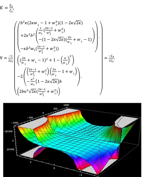
curvatures as follows 𝐾 =8* P+, 𝐻 =%43" % ⎝ ⎜ ⎜ ⎜ ⎜ ⎜ ⎜ ⎜ ⎜ ⎜ ⎜ ⎜ ⎜ ⎛ ⎝ ⎜ ⎜ ⎜ ⎛ 𝑏%𝜅(2𝜅𝑤 !− 1 + 𝑤 !*)(1 − 2𝜅√2𝜅) +2𝜅%𝑏%X " #!( %,3" # !% + 𝑤 %!) −(1 − 2𝜅√2𝜅)(#%, !+ 𝑤 !− 1) Y −𝜅𝑏%𝑤 "(%,3"# !% + 𝑤 ! %)) ⎠ ⎟ ⎟ ⎟ ⎞ . K(#%, !+ 𝑤 !− 1) %+ 1 − N, # !O % L −2 ZN %,3" # !% + 𝑤 %!O N#%, !− 1 + 𝑤 !O −#,% ![1 − 2𝜅√2𝜅\𝑏 ] . N2𝑏𝜅%√2𝜅(%,3" # !% + 𝑤 %!)O ⎠ ⎟ ⎟ ⎟ ⎟ ⎟ ⎟ ⎟ ⎟ ⎟ ⎟ ⎟ ⎟ ⎞ =3&( %4%.
Figure 1: The α − magnetic surface formed by the 𝑊! trajectory
4.1. The Clairaut’s Theorem on magnetic surface generated by 𝛂 −magnetic curve in 𝐐𝟐⊂ 𝑬
𝟏 𝟑
In this section, Clairaut’s theorem is given on magnetic surface generated by 𝛼 −magnetic curve in 𝐐%⊂ 𝐸
$#. Also, the general equations of geodesics on surface formed by an 𝛼 −magnetic
curve in 𝐐% are expressed.
1. For ℎ(𝜉) =constant, the following equation supplies 0 = ⎝ ⎜ ⎜ ⎛ ( )!"(sinh %(𝑤 "𝜉) + cosh%(𝑤"𝜉)) − 2(5 $ )!"+ 𝑓)sinh(𝑤"𝜉) −2cosh(𝑤"𝜉)(5 $ )!+ 5 #!%) + √% % sin[2√2𝜉\ + 𝑔 )cos[√2𝜉\ −√2𝑔sin[√2𝜉\ + 2(" )!*+ " )!)sinh(2𝑤"𝜉) + 𝑓𝑓)+ 𝑔𝑔)⎠ ⎟ ⎟ ⎞ .
Hence, the Lagrange equation on the magnetic surface 𝛬*(𝜉, 𝑡) is given by
𝐸(𝜉, 𝑡)𝜉.%+ 𝐺(𝜉)𝑡.%= 𝐿.
2. The curve 𝛿(𝑠) = 𝛬*(𝜉(𝑠), 𝑡(𝑠)) is a geodesic on the surface 𝛬*(𝜉, 𝑡) if and only if the
following equations satisfy
𝜉 = ∫<23RGHAQ𝑑𝑠 + 𝑐S‘or 𝜉 = ∫<23RGHAQ𝑑𝑠’ , 2 ∫ 𝐸(𝜉, 𝑡)𝑑𝜉 = 𝑐9𝑠 + 𝑐T,
0 = 2𝐺(𝜉)𝑡. − ª∫.M(8,2).2 𝜉.𝑑𝑠 + 𝑐:«,
or
𝑡 = ∫ sin𝜃𝑑𝑠(or 𝑡 = ∫ sin𝜃𝑑𝑠 + 𝑐#), 𝑡 =%N(8)V&' + 𝑐%,
2𝐸(𝜉, 𝑡)𝜉.. = 𝐺8𝑡.%− 𝐸 8𝜉
. %,
where 𝑐W ∈ ℝ,.
Proof. Let ΛX(ξ, t) be the magnetic surface generated by α −magnetic curve and let
δX(t): I ⊂ ℝ → 𝐐% be a regular curve in 𝐐% are parametrized by
𝛬!(𝜉, 𝑡) = ⎝ ⎜ ⎛ (%,6789(#!&) )!" + %,<=69(#!&) #! + 𝑓(𝜉))(𝑎𝑡 + 𝑏), (𝑐𝑜𝑠ℎ(√2𝜅𝜉) + 𝑔(𝜉))(𝑎𝑡 + 𝑏), (,>#)!+ ! − 2𝜅 %𝑠𝑖𝑛ℎ(√2𝜅𝜉) + ℎ(𝜉))(𝑎𝑡 + 𝑏)); ⎠ ⎟ ⎞ , where 𝑓(𝜉) = −1 − 8 0 &+ − 8+ %! + 𝑤$𝑒0&8+ :=+8. 9! + ⋯, (9) 𝑔(𝜉) =%=0&+8/ :! +. . . ; ℎ(𝜉) = ;:(=0&)+8. 9! +. ...
Λ!&= ⎩ ⎪ ⎪ ⎪ ⎨ ⎪ ⎪ ⎪ ⎧ ZT %,$ )!"+ 2𝜅U sinh(𝑤"𝜉) + T%, )!%+ %,$ )!U cosh(𝑤"𝜉) + 𝑓)(𝜉) ] (𝑎𝑡 + 𝑏), KT√2𝜅 +√%,%√,$𝜉U sinh(√2𝜅𝜉) + 𝑔)(𝜉)L (𝑎𝑡 + 𝑏), M−4𝜅𝜅 )sinh(√2𝜅𝜉) −2𝜅)T√2𝜅 +√%,$ %√,𝜉U cosh(√2𝜅𝜉) + ℎ )(𝜉)P (𝑎𝑡 + 𝑏) ⎭ ⎪ ⎪ ⎪ ⎬ ⎪ ⎪ ⎪ ⎫ = (𝑎𝑡 + 𝑏)𝑁&, Λ*2 = ⎝ ⎜ ⎛( %=ABCD(0&8) (&* + %=GHAD(0&8) 0& + 𝑓(𝜉))𝑎, (cosh(√2𝜅𝜉) + 𝑔(𝜉))𝑎, (=I (&-0& − 2𝜅 %sinh(√2𝜅𝜉) + ℎ(𝜉))𝑎); ⎠ ⎟ ⎞ = 𝑁2. Hence, we have 𝐸(𝜉, 𝑡) = (𝑎𝑡 + 𝑏)% ⎝ ⎜ ⎜ ⎜ ⎛ 𝐴%sinh%(𝑤 $𝜉) + 2𝐴sinh(𝑤$𝜉)`𝐵cosh(𝑤$𝜉) + 𝑓"(𝜉)c +𝐵%cosh%(𝑤 $𝜉) + 2𝐵cosh(𝑤$𝜉)𝑓"(𝜉) + 𝑓"%(𝜉) +(𝐶%− 16𝜅%𝜅")sinh%`√2𝜅𝜉c + 2𝐶sinh`√2𝜅𝜉c𝑔"(𝜉) +𝑔"%(𝜉) + 8𝜅𝜅"sinh`√2𝜅𝜉c ‘ℎ"(𝜉) − 2𝜅"𝐶cosh`√2𝜅𝜉c’ −ℎ"%(𝜉) + 4𝜅"𝐶cosh`√2𝜅𝜉c − 4𝜅"%𝐶%cosh%`√2𝜅𝜉c ⎠ ⎟ ⎟ ⎟ ⎞ , 𝐸(𝜉, 𝑡) = 𝑃(𝑡)𝑁(𝜉), where 𝐴 =%=# (&*+ 2𝜅, 𝐵 = %= (&++ %=# (&, 𝐶 = √2𝜅 + √%=# %√= 𝜉. 𝐺(𝜉) = 𝑎 ⎝ ⎜ ⎜ ⎛ :=+ 0&4sinh %(𝑤 $𝜉) + %= (&*sinh(𝑤$𝜉) ‘ %= (&cosh(𝑤$𝜉) + 𝑓(𝜉)’ +:=+ 0&+cosh %(𝑤 $𝜉) + :=(&𝑓(𝜉)cosh(𝑤$𝜉) + 𝑓%(𝜉) +cosh%(√2𝜅𝜉) + 2𝑔(𝜉)cosh(√2𝜅𝜉) + 𝑔%(𝜉) −4𝜅:sinh%(√2𝜅𝜉) + 4𝜅%sinh(√2𝜅𝜉)ℎ(𝜉) − ℎ%(𝜉) ⎠ ⎟ ⎟ ⎞ , (10)
for the following equation ℎ(𝜉) = constant, 0 =⎜⎜ ⎛ : (&*(sinh %(𝑤 $𝜉) + cosh%(𝑤$𝜉)) −2 ‘Y#
(&*+ 𝑓’ sinh(𝑤$𝜉) − 2cosh(𝑤$𝜉) ‘ Y# (&+
Y 0&+’
+√%sin`2√2𝜉c + 𝑔"cos`√2𝜉c − √2𝑔sin`√2𝜉c ⎟
⎟ ⎞
where for the 𝛼 −magnetic curve, we have 𝜅 = −1, $
(&= 𝑐, we obtain 𝐹(𝜉) = 0. Thus, the first
fundamental form is given by
𝐼 = “𝐸(𝜉, 𝑡) 00 𝐺(𝜉)”. (12)
Moreover, it is important to note that, the coordinates of parametrization are orthogonal, since the first fundamental form is diagonal. So, from the first fundamental form, we have the Lagrangian equation given by
𝐸(𝜉, 𝑡)𝑑%𝜉 + 𝐺(𝜉)𝑑%𝑡 = 𝐿 or 𝐸(𝜉, 𝑡)𝜉.%+ 𝐺(𝜉)𝑡.% = 𝐿, (13)
and a geodesic on the surface Λ*(𝜉, 𝑡) is given by the Euler-Lagrangian equations,
𝜕 𝜕𝑠• 𝜕𝐿 𝜕𝜉 𝜕𝑠 – =𝜕𝐿 𝜕𝜉; 𝜕 𝜕𝑠• 𝜕𝐿 𝜕𝑡 𝜕𝑠 – =𝜕𝐿 𝜕𝑡.
i) For the equation
2𝐸(𝜉, 𝑡)𝜉.. = 𝐺8𝑡.%− 𝐸 8𝜉
.
%, (14)
and from the equation .'. g./'5 '$
h =./.2= 0, we obtain .'. `2𝐺(𝜉)𝑡.c = 0, which means 2𝐺(𝜉)𝑡. is constant along the geodesic and we have
𝑡 = V&'
%N(8)+ 𝑐%. (15)
Let 𝛿* be a geodesic on the surface Λ*(𝜉, 𝑡), so the curve is written as (𝜉(𝑠), 𝑡(𝑠)), also let
𝜃 be the angle between 𝛿.* and a meridian and 𝑁8 is the vector pointing along meridians of Λ* and
𝑁2 is the vector pointing along meridians of Λ*. We can say that {𝑁8, 𝑁2} orthonormal basis and
hence a unit vector 𝛿. tangent to Λ*(𝜉, 𝑡) can be written by
𝛿. = 𝜉.Λ* -+ 𝑡.Λ 5 * = 𝑁 8cos𝜃 + 𝑁2sin𝜃 = 𝜉 . (𝑎𝑡 + 𝑏)𝑁8 + 𝑡.𝑁2.
We see that 𝑡. = sin𝜃, hence we write
being a constant along 𝛿*. On the contrary, let 𝛿 be 𝛼 −magnetic curve with 2𝐺(𝜉)𝑡. = 2𝐺(𝜉)sin𝜃 is a constant. Hence, the second Euler-Lagrange equation is satisfied,
differentiating 𝐿 and substituting this into the first equation yields the first Euler-Lagrange equation. Furthermore, we can also write
𝑡 = ∫ sin𝜃𝑑𝑠 or 𝑡 = ∫ sin𝜃𝑑𝑠 + 𝑐#. (17)
ii) For the equation
2𝐺(𝜉)𝑡. − ª∫.M(8,2).2 𝜉.𝑑𝑠 + 𝑐:« = 0, (18)
from the equation .'. g./'( '$
h =.0./ = 0, we obtain '(./ '$
= 2𝐸(𝜉, 𝑡)𝜉. is constant and which means
2 ∫ 𝐸(𝜉, 𝑡)𝑑𝜉 = 𝑐9𝑠 + 𝑐T,
which has a constant along the geodesic. We see that (𝑎𝑡 + 𝑏)𝜉. = cos𝜃, hence we write
2𝐸(𝜉, 𝑡)𝜉. =%M(8,2)
<23R cos𝜃, (19)
being a constant along 𝛿*. On the contrary, 𝛿* is a curve with 2𝐸(𝜉, 𝑡)𝜉. =%M(8,2)
<23R cos𝜃 that it is a
constant. Hence, the first Euler-Lagrange equation is satisfied, differentiating 𝐿 and substituting this into the second equation yields the second Euler-Lagrange equation. Furthermore, we can write equation as follows
𝜉 = ∫ <23RGHAQ𝑑𝑠 or 𝜉 = ∫<23RGHAQ𝑑𝑠 + 𝑐S. (20)
Theorem 7. The general equations of geodesics on the surface generated by an
𝛼 −magnetic curve in 𝑸% are given by
i) For the parameter 𝜉 = ∫<23RVZ'Q𝑑𝑠 + 𝑐S (or 𝜉 = ∫ <23RVZ'Q𝑑𝑠) and the equations
2 ∫ 𝐸(𝜉, 𝑡)𝑑𝜉 = 𝑐9𝑠 + 𝑐T, 2𝐺(𝜉)𝑡 .
− ª∫.M(8,2).2 𝜉.𝑑𝑠 + 𝑐:« = 0, the following equation holds
𝑑𝑡 𝑑𝜉= 𝑐$$· 𝐸(𝜉, 𝑡) 𝐺(𝜉) ¸𝐿𝐸(𝜉, 𝑡) − 𝑐$,= 𝑎𝑡 + 𝑏 ¸𝐺(𝜉)cos𝜃·𝐿 − 𝐸(𝜉, 𝑡)cos%𝜃 𝑎𝑡 + 𝑏 .
𝑑𝜉 𝑑𝑡 = 𝑐$𝐺(𝜉)· 𝐺(𝜉)𝜀 − 𝑐% 𝐸(𝜉, 𝑡)𝐺(𝜉)= 1 𝑠𝑖𝑛𝜃· 𝜀 − 𝐺(𝜉)𝑠𝑖𝑛%𝜃 𝐸(𝜉, 𝑡) , where 𝑐W ∈ ℝ,, 𝑖 ∈ 𝐼.
Proof. In order to obtain the general equation of geodesics, we should use the Euler
Lagrange equations,
i) For the parameters 𝜉 = ∫ <23RGHAQ𝑑𝑠 + 𝑐S (or 𝜉 = ∫<23RGHAQ𝑑𝑠) and the equations 2 ∫ 𝐸(𝜉, 𝑡)𝑑𝜉 = 𝑐9𝑠 + 𝑐T, 2𝐺(𝜉)𝑡. − ª∫.M(8,2).2 𝜉.𝑑𝑠 + 𝑐:« = 0, we have . .'g ./ '5 '$ h =./ .2 ≠ 0 and . .'g ./ '-'$ h =./
.8= 0. From the solving of the second Lagrangian
equation, we get .'. ‘2𝐸(𝜉, 𝑡)𝜉.’ = 0, which means (8(' = V. %M(8,2).
If we put the value of 𝜉. at 𝐸(𝜉, 𝑡)𝜉.%+ 𝐺(𝜉)𝑡.%= 𝐿,
𝐸(𝜉, 𝑡) ‘(8('’%+ 𝐺(𝜉) ‘(8(2(8('’%= 𝐿, (21)
we obtain the general equation of geodesics on Λ*(𝜉, 𝑡) as follow
(2 (8 = 𝑐$$º M(8,2) N(8) ¸𝐿𝐸(𝜉, 𝑡) − 𝑐$, 𝑜𝑟 (2 (8= <23R [N(8)GHAQº𝐿 − M(8,2)GHA+Q <23R . (22)
ii) For the parameters 𝑡 = ∫ sin𝜃𝑑𝑠 (or 𝑡 = ∫ sin𝜃𝑑𝑠 + 𝑐\) or 𝑡 =%N(8)V.' + 𝑐T and the
equation 2𝐸(𝜉, 𝑡)𝜉.. = 𝐺8𝑡 . %− 𝐸 8𝜉 . %, (23) since . .'g ./ '-'$ h =./
.8≠ 0 and from the solving of the differential equations in . .'g ./ '5 '$ h =./ .2= 0, 𝑡. = sin𝜃 or 𝑡. = V& %N(8),
(2 (' =
V&
%N(8). (24)
If we put the value of 𝑡. at 𝐸(𝜉, 𝑡)𝜉.%+ 𝐺(𝜉)𝑡.%= 𝐿,
𝐸(𝜉, 𝑡) ‘(8 (2 (2 ('’ % + 𝐺(𝜉) ‘(2 ('’ % = 𝐿, (25)
we can obtain the general equation of geodesics on Λ*(𝜉, 𝑡) as follow
(8 (2 = 𝑐$𝐺(𝜉)º N(8)/;V+ M(8,2)N(8) 𝑜𝑟 (8 (2 = $ ABCQº /;N(8)ABC+Q M(8,2) . (26)
5. The Physical Approach on 𝜶 −magnetic Surface in 𝐐𝟐⊂ 𝑬 𝟏 𝟑
In this section, we try to express as the point of view of a physicist to imagine tracing out a geodesic by determining the affine parameter 𝑠 with the time, thinking that the picture is now of a point particle that is moving on the surface, tracing out a path called the orbit of the particle.
Let Λ*(𝜉(𝑠), 𝑡(𝑠)) be a parametrized curve on surface as
Λ*(𝜉(𝑠), 𝑡(𝑠)) = ⎝ ⎜ ⎛( %=ABCD(0&8) (&* + %=GHAD(0&8) 0& + 𝑓(𝜉))(𝑎𝑡 + 𝑏), (cosh(√2𝜅𝜉) + 𝑔(𝜉))(𝑎𝑡 + 𝑏), (=I (&-0& − 2𝜅 %sinh(√2𝜅𝜉) + ℎ(𝜉))(𝑎𝑡 + 𝑏)) ⎠ ⎟ ⎞ .
Also, the Lagrange equation on Λ*(𝜉, 𝑡) the magnetic surface is given as follows
𝐸(𝜉, 𝑡)𝜉.%+ 𝐺(𝜉)𝑡.%= 𝐿.
Furthermore, the tangent vector to this curve can be obtained using the chain rule as follow
𝛿. =(J0(8('),2(')) (' = (8(') (' Λ* -+ (2(') (' Λ* 5= 𝑁8cos𝜃 + 𝑁2sin𝜃 = 𝜉.Λ* -+ 𝑡 . Λ* 5= 𝜉 . (𝑎𝑡 + 𝑏)𝑁8 + 𝑡 . 𝑁2. (27)
Hence, we can write the tangent vector of the geodesic curve as follows
𝑌›⃗ =(J0(8('),2('))(' = 𝑌8Λ -* + 𝑌2Λ
5
of change of the arc length along the curve 𝛿. Think that 𝑌8∗
= ¸𝐸(𝜉, 𝑡)𝑌8 = 𝑌cos𝜃 is just the
radial velocity while 𝑌8 is the horizontal angular velocity and 𝑌2∗ = ¸𝐺(𝜉)𝑌2 = 𝑌sin𝜃 is the
vertical component of the velocity vector. Hence, we can give the velocity in terms of polar coordinates in the tangent plane to explain its magnitude and slope angle according to the radial direction on the surface.
The role of the radial variable on this velocity plane is played by the speed, here we can say that the direction of the velocity according to the direction Λ* 5∗ on this plane is given by the
angle 𝜃. Also, we can say that the speed is constant along the geodesic. In [20, 21], to find out the system of two second order geodesic equations it is expressed that a standard physics technique of partially can be used integrating them by anyone and so lessen them to two first order equations by taking two constants of the movement that it comes out from the two independent symmetries of the equations of movement. Those physical properties as energy and momentum are replaced by the specificquantities found by partitioning out the mass. Therefore, we can write the specific kinetic energy as follows
𝐸 =$ %𝑌%= $ %𝐸(𝜉, 𝑡) ‘ (8 ('’ % +$ %𝐺(𝜉) ‘ (2 ('’ % =$ %(𝑌%cos%𝜃 + 𝑌%sin%𝜃), (29)
using the right side of the previous equations we can say that both the specific energy and speed have to be constant along geodesic.
In the point of view of the physics, the specific kinetic energy of the particle is constant because of its motion in space, and only accelerates perpendicular to the surface. If a force is accountable for this acceleration, that is to say that the normal force that it supplies the particle on the surface, because of perpendicular to the velocity of the particle it wouldn’t study on the particle. Therefore, the specific energy 𝐸 has to be constant. Resembling, we say that the speed 𝑌 = √2𝐸 is constant along a geodesic in respect of this cause.
Theorem 8. Let 𝛬*(𝜉, 𝑡) be the magnetic surface generated by 𝛼 −magnetic curve. Then
the specific kinetic energy of the particle on the 𝛼 −magnetic surface 𝛬*(𝜉, 𝑡) is constant under
evident conditions and the following statements are held:
1. For the parameter 𝑡 = ∫ 𝑠𝑖𝑛𝜃𝑑𝑠 ‘or 𝑡 = V&'
%N(8)+ 𝑐%’ and the equation 2𝐸(𝜉, 𝑡)𝜉 ..
= 𝐺8𝑡.%− 𝐸
8𝜉 .
%, the specific angular momentum ℓ
ℓ$= ¸𝐺(𝜉)𝑌sin𝜃; 𝐸$=$ %“𝐸(𝜉, 𝑡) ‘ (8 ('’ % + ℓ&+ N(8)”. (30)
2. For the parameter 𝜉 = ∫<23RVZ'Q𝑑𝑠 and the equations 2 ∫ 𝐸(𝜉, 𝑡)𝑑𝜉 = 𝑐9𝑠 + 𝑐T,
2𝐺(𝜉)𝑡. − ª∫.M(8,2).2 𝜉.𝑑𝑠 + 𝑐:« = 0, the specific angular momentum ℓ% and specific kinetic
energy 𝐸% are constant along a geodesic, and are given as follows
ℓ%= −¸𝐸(𝜉, 𝑡)𝑌𝑐𝑜𝑠𝜃; 𝐸% =$ %“ ℓ++ M(8,2)+ 𝐺(𝜉) ‘ (2 ('’ % ”, (31)
where 𝑐W ∈ ℝ,, and 𝑌 is the tangent vector of the geodesic curve.
Proof. 1) For the equation t = ∫ sinθds ‘or t = G&A
%a(b)+ c%’ and the equation 2E(ξ, t)ξ ..
= Gbt.%− E
bξ .
%, we write 2G(ξ)t. = 2G(ξ)sinθ being a constant along δ and by using this situation
we explain in this physics language. Also, we can explain as to circular motion around an axis with radius Á𝑅››››⃗Á = ¸G(ξ) or 𝑅$ ››››⃗ = ¸G(ξ)𝑒$ ›››⃗, namely the velocity Y$ c∗= ¸G(ξ)Yc = Ysinθ =
¸G(ξ)dc
dA in the angular direction multiplied by the radius ¸G(ξ) of the circle. Physically, the
specific angular momentum ℓ$ can be written as following equation
ℓ$= 𝑒›››⃗ . `𝑅# ››››⃗ ×$ N*Y››⃗c = ¸𝐺(𝜉)𝑌sin𝜃, (32)
since 𝑌2∗
= 𝑌sin𝜃 = ¸𝐺(𝜉)(2
(', we can write ¸𝐺(𝜉)𝑌sin𝜃 = 𝐺(𝜉) (2
(' being a constant along
𝛿(𝜉), and we say that the specific angular momentum ℓ$ is constant along a geodesic and we get
ℓ$= 𝐺(𝜉)(2 ('⇒ (2 ('= ℓ& N(8). (33)
This expression can be rewritten the changeable angular velocity 𝑑𝑡/𝑑𝑠 in the specific energy formula according to the constant angular momentum, the specific energy 𝐸$ is given as
𝐸$=$ %(𝐸(𝜉, 𝑡) ‘ (8 ('’ % + ℓ&+ N(8)). (34)
2) For the parameter 𝜉 = ∫<23RGHAQ𝑑𝑠 and the equations 2 ∫ 𝐸(𝜉, 𝑡)𝑑𝜉 = 𝑐9𝑠 + 𝑐T,
2𝐺(𝜉)𝑡. − ª∫.M(8,2).2 𝜉.𝑑𝑠 + 𝑐:« = 0, we write 2𝐸(𝜉, 𝑡)𝜉. = 2𝐸(𝜉, 𝑡)cos𝜃 being a constant along 𝛿(𝜉) and by using this situation we explain in this physics language. Also, we can express as in
multiplied by the radius ¸𝐸(𝜉, 𝑡) of the circle. The first geodesic equation is told that the specific angular momentum is constant along a geodesic, and the specific angular momentum ℓ% can be
taken down as following equation
ℓ%= 𝑒›››⃗ . `𝑅# ››››⃗ ×% N*Y››⃗c = −¸𝐸(𝜉, 𝑡)𝑌cos𝜃, (35)
since ¸𝐸(𝜉, 𝑡)(8
(' = 𝑌cos𝜃, we can write −𝐸(𝜉, 𝑡) (8
(' = −¸𝐸(𝜉, 𝑡)𝑌cos𝜃, and we say that the
specific angular momentum is constant along a geodesic. So, we have
ℓ%= −𝐸(𝜉, 𝑡)(8 (' ⇒ (8 (' = ;ℓ+ M(8,2). (36)
Hence, this statement can be rewritten the changeable angular velocity 𝑑𝜉/𝑑𝑠 in the specific energy formula according to the constant angular momentum specific energy 𝐸% is given
by 𝐸% =$ %“ ℓ++ M(8,2)+ 𝐺(𝜉) ‘ (2 ('’ % ”. (37) 6. Conclusion
In this study, the 𝛼 −magnetic surfaces constituted by using the 𝛼 −magnetic curves to be geodesics on the surface are expressed. The 𝛼 −magnetic surfaces generated by the 𝛼 −magnetic curves are examined, and some certain results of describing the geodesics are given on the surfaces. Our results show that the specific energy and specific angular momentum obtained on the 𝛼 −magnetic surfaces can be expressed in 𝐐%. The physical meanings of specific energy and
specific angular momentum are of course related with the physical meaning itself. First of all, the conditions of being geodesic of the curves selected as magnetic curves are examined, and these geodesic conditions allows us to express the specific energy. We are working on the properties of these surfaces with a view to devising suitable metric in 𝐐%. It is hoped that researches will benefit
from this study about the rotated surface.
Acknowledgement
The authors wish to express their thanks to the authors of literatures for the supplied scientific aspects and idea for this study. Furthermore, we request to explain great thanks to reviewers for the constructive comments and inputs given to improve the quality of our work.
References
[1] Almaz, F., Kulahci, M.A., A survey on magnetic curves in 2-dimensional lightlike cone, Malaya Journal of Matematik, 7(3), 477-485, 2019.
[2] Asperti, A., Dajezer, M., Conformally Flat Riemannian Manifolds as Hypersurface of
the Light Cone, Canadian Mathematical Bulletin, 32, 281-285, 1989.
[3] Barros, M., Cabrerizo, M.F., Romero, A., Magnetic Vortex Filament Flows, Journal of Mathematical Physics, 48, 1-27, 2007.
[4] Barros, M., Romero, A., Magnetic Vortices, Europhysics Letters, 77, 1-5, 2007. [5] Sunada, T., Magnetic Flows on a Riemannian Surface, In Proceedings of KAIST Mathematics Workshop, 93-108, 1993.
[6] Bozkurt, Z., Gök, İ., Yaylı, Y., Ekmekci, F.N., A new approach for magnetic curves in
Riemannian 3D-manifolds, Journal of Mathematical Physics, 55, 1-12, 2014.
[7] Bejan, C.L., Druta-Romaniuc, S.L., Walker manifolds and Killing magnetic curves, Differential Geometry and its Applications, 35, 106-116, 2014.
[8] Kruiver, P.P., Dekkers, M.J., Heslop, D., Quantification of magnetic coercivity
componets by the analysis of acquisition, Earth and Planetary Science Letters, 189(3-4), 269-276,
2001.
[9] Munteanu, M.I., Nistor, A.I., A note magnetic curves on 𝑆%e3$, Comptes Rendus de
l'Académie des Sciences - Series I, 352, 447-449, 2014.
[10] Brinkmann, W.H., On Riemannian spaces conformal to Euclidean space, Proceedings of the National Academy of Sciences of the United States of America, 9, 1-3, 1923.
[11] Kuhnel, W., Differential geometry curves- surfaces and manifolds, American Mathematical Society, Second Edition, United States of America, 2005.
[12] Kulkarni, D.N., Pinkall, U., Conformal geometry, A Publication of the Max-Planck-Institut für Mathematik, Bonn, Aspects of Mathematics, 12, 1988.
[13] Pressley, A., Elementary differential geometry, Springer Undergraduate Mathematics Series, Second Edition, Springer-Verlag London, 2010.
[14] Calvaruso, G., Munteanu, M.I., Perrone, A., Killing magnetic curves in
three-dimensional almost paracontact manifolds, Journal of Mathematical Analysis and Applications,
426, 423-439, 2015.
[15] Druta-Romaniuc, S.L., Munteanu, M.I., Killing magnetic curves in a Minkowski
3-space, Nonlinear Analysis Real World Applications, 14, 383-396, 2013.
[16] Kulahci, M., Bektas, M., Ergüt, M., Curves of AW(k)-type in 3-dimensional null cone, Physics Letters A, 371, 275-277, 2007.
[17] Kulahci, M., Almaz, F., Some characterizations of osculating in the lightlike cone, Boletim da Sociedade Paranaense de Matematica, 35(2), 39-48, 2017.
[18] Liu, H., Curves in the lightlike cone, Contributions to Algebra and Geometry, 45(1), 291-303, 2004.
[21] Walecka, J.D., Topics in modern physics: theoretical foundations, World Scientific, 2013.
[22] Lerner, D., Lie derivatives, ısometries, and Killing vectors, Department of Mathematics, University of Kansas, Lawrence, Kansas, 66045-7594, 2010.