Selçuk J. Appl. Math. Selçuk Journal of Vol. 11. No.2. pp. 103-108, 2010 Applied Mathematics
On Canal Surfaces in3
G. Öztürk1, B. Bulca2, B. K. Bayram3, K. Arslan4
Department of Mathematics Kocaeli University 41380 Kocaeli, Türkiye e-mail: 1ogunay@ ko caeli.edu.tr
24Department of Mathematics Uludag University 16059 Bursa, Türkiye
e-mail: 2bbulca@ uludag.edu.tr,4arslan@ uludag.edu.tr
Department of Mathematics Balıkesir University Balıkesir, Türkiye e-mail: 3b enguk@ balikesir.edu.tr
Received Date: February 10, 2010 Accepted Date:May 3, 2010
Abstract. In this paper we deal with the geometric properties of canal surfaces in E3. Further, the first and second fundamental form of canal surfaces are presented. By the use of the second fundamental form, the Gaussian and mean curvature of canal surfaces are obtained. Finally, the visualization of canal surfaces which their spine curves are unit circle and a straight line are presented. Key words: Canal surface, Gaussian curvature, mean curvature.
2000 Mathematics Subject Classification. 53A04, 53C42. 1. Introduction
A canal surface is defined as envelope of a one-parameter set of spheres, centered at a spine curve () with radius (): When () is a constant function, the canal surface is the envelope of a moving sphere and is called a pipe surface. Canal surfaces have wide applications in CAGD, such as construction of blend-ing surfaces, shape reconstruction, transition surfaces between pipes, robotic path planning, etc. (see, [1], [2], [3]). Most of the literature on canal surfaces within the CAGD context has been motivated by the observation that canal surfaces with rational spine curve and rational radius function is rational, and it is therefore natural to ask for methods which allow one to construct a rational parametrization of canal surfaces from its spine curve and radius function. The developable surface plays a important role in CAGD. It is well known that, at regular points, the Gaussian curvature of a developable surface is identically zero. In [3] it has been proved that developable canal surface is either a cylinder or a cone.
The paper is organized as follows. In section 2, we shall discuss geometric properties of canal surfaces. The first and second fundamental forms of canal surfaces are presented. By the second fundamental form, the Gaussian and mean curvature of canal surfaces are given. In section 3, the visualization of canal surfaces which their spine curves are unit circle and a straight line are presented. All the figures in this paper were created using Maple programme. 2. Canal Surfaces
Recall definitions and results of [5]. In the present section we will consider canal surfaces in E3 Canal surface is a surface formed as the envelope of a family of spheres whose centers lie on a space curve.
Let () = (1() 2() 0) be a plane curve parametrized by arclength. The corresponding Frenet formulas have the following form:
(2.1)
0() = 1() 10() = ()2() 20() = −()1()
where 1() and 2() are the tangent and normal vectors of the curve re-spectively. We choose a constant vector 3() of E3. The canal surface of the planar curve has the following parametrization (see, [6]):
(2.2) : ( ) = () + () (2() cos + 3() sin )
where () is the radius of the spheres from the definition of the canal surface. The tangent space to at an arbitrary point = ( ) of is spanned by (2.3) ( ) = (1 − cos )1+ (
0cos )2+ (0sin )3 ( ) = −( sin )2+ ( cos )3
Further, the coefficients of the first fundamental form become
(2.4)
= h i = (0)2+ (1 − cos )2 = h i = 0
= h i = 2 The unit normal vector field of is
(2.5)
= × k× k = 1
{01− cos (1 − cos )2− sin (1 − cos )3} where 2= − 2
The second partial derivatives of ( ) are expressed as follows:
(2.6)
= − cos (20 + 0)1+( − 2
cos + 00cos )
2+(00sin )3 = ( sin )1− (0sin )2+ (0cos )3
Further, the coefficients of the second fundamental form become, (2.7) = = 1 {cos (−2(0) 2 − 200− + 200 sin2) + cos2(222) + cos3(200 − 33) − 00} = = 20 sin = = 2− 3 cos
The Gaussian and mean curvature of a regular patch are given by
(2.8) = − 2 − 2 (2.9) = + − 2 2( − 2) respectively (see, [6]).
Summing up the following results are proved.
Theorem 2.1. Let be a canal surface in E3given with the parametrization (2.2). Then the Gaussian and mean curvatures of at point are
(2.10) = 3 4{ cos (2 00 − 00−2(0)2 − ) + cos2(3(0)2 2+200+32 −2002) + cos3(−32 3)+ cos4(3 4) − 00−(0)2 2} and (2.11) = 2 23{cos ( 200 − 3(0)2 − 200− 4) + cos2(522) + cos3(−233) − 00+ 1 + (0)2}
Corollary 2.1. Let be a pipe surface (i.e. () is a constant function) in E3given with the parametrization (2.2). Then the Gauss and mean curvatures of at a point are
= cos
(1 − cos )4{− + (3 2
) cos − (323) cos2 + (34) cos3}
= 1
2(1 − cos )3{1 − (4) cos + (5
22) cos2
Corollary 2.2. Let be a canal surface in E3given with the parametrization (2.2). If the spine curve is a straight line then the Gauss and mean curvatures of at a point are (2.12) = −00 (1 + (0)2)2 (see, [6]) and (2.13) =−00+ (0) 2+ 1 2(1 + (0)2)32
Example 2.1. Consider the unit circle () = (cos sin 0) in E3 Then the canal surface of the spine curve in E3 has the following parametrization (2.14)
( ) = ( cos () − () cos ()() sin () − () sin () cos () () sin ())
Example 2.2. Consider the straight line () = (1 + 1 2 + 2 0) in E3 where 2
1+ 22 = 1 Then the canal surface of the spine curve in E3 has the following parametrization
(2.15)
( ) = (1 + 1−2() cos () 2 + 2+1() cos () () sin ()) where 1 1 2 2 are real constants.
3. Visualization
We visualize the surfaces given with the patch ( ) = (( ) ( ) ( )) making use of Maple. Furthermore, we plot the graph of the given surface by using maple plotting command
(3.1) 3([ ] = = );
In the sequel we construct some 3D geometric shape models of canal surfaces. First, we construct the geometric model of the canal surface given in Example 2.1 We visualize some surface models of the patch (2.14) using the following values respectively (see Figure 1) ;
(3.2)
) () = ) () = 2 ) () = sin
Figure 1. The canal surfaces of a unit circle
Secondly, we construct the geometric model of the canal surface given in Exam-ple 2.2. We visualize some surface models of the patch (2.15) using the values 1= 45; 2= 35; 1= 4; 2= 5 and () given in (3.2) respectively (see Figure 2);
Figure 2. The canal surfaces of a straight line
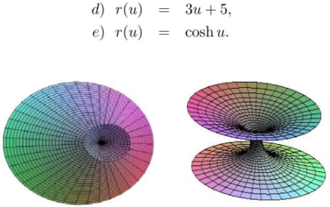
Finally, we visualize the graph of the flat and minimal canal surfaces given by (2.15) using the following values of () respectively, (see Figure 3);
) () = 3 + 5 ) () = cosh
4. Conclusion
In this paper, a method of canal surfaces is investigated. For demonstrating the performance of the proposed method, parameters of canal surfaces models were constructed from the spine curve . Infect, canal surfaces are solid models that can fairly simple parametrization of representing a large variety of standard geometric models. They have wide applications in CAGD, such as construction of blending surfaces. This makes them much more convenient for representing shape reconstruction, transition surfaces and pipe surfaces. By the use of main results of differential geometry we calculated the Gaussian and mean curvatures of canal surfaces in E3 Moreover, this frame work can be used for the modelling of 3-D shapes in E3. For future work it will be necessary to improve the system to allow for the canal surface in E4
References
1. Farouki, R.A. and Sverrissor, R., Approximation of Rolling-ball Blends for Free-form Parametric Surfaces, Computer-Aided Design 28,871-878, (1996).
2. Wang, L., Ming, C.L., and Blackmore, D., Generating Swept Solids for NC Ver-ification Using the SEDE Method, Proceedings of the Fourth Symposium on Solid Modeling and Applications, Atlanta, Georgian, May 14-16,364-375. (1997)
3. Xu, Z., Feng, R. and Sun, JG., Analytic and Algebraic Properties of Canal Sur-faces, Journal of Computational and Applied Mathematics, Volume 195, Issues 1-2, 15 October 2006, Pages 220-228.
4. Shani, U. and Ballard, D.H., Splines as Embeddings for Generalized Cylinders, Computer Vision,Graphics and Image Processing 27,129-156, (1984).
5. Gray, A. Modern Differential Geometry of Curves and Surfaces. CRC Press, Boca Raton Ann Arbor London Tokyo, (1993).
6. Gal, R.O. and Pal, L.Some Notes on Drawing Twofolds in 4-dimensional Euclidean space, Acta Univ. Sapientiae, Informatica, 1, 2, 125—134, (2009).