APPLICATION OF BOOTSTRAP METHODOLOGY IN
FUND PERFORMANCE
EL F ÇAKMAKO LU
106626008
STANBUL B LG UNIVERSITY
INSTITUTE OF SOCIAL SCIENCES
FINANCIAL ECONOMICS – QUANTITATIVE FINANCE
PROF. DR. BURAK SALTO LU
2010
Application of Bootstrap Methodology in Fund Performance
Elif Çakmako5lu
106626008
Prof. Dr. Burak Salto5lu:
Assoc. Prof. Dr. Ege Yazgan
Asst. Prof. Dr. Orhan Erdem
Date of Approval:
June 9, 2010
Number of Pages:
98
Keywords (English)
Keywords (Turkish)
1) Bootstrap
1) Bootstrap
2) Alpha
2) Alfa
3) Performance Measurement 3) Performance Ölçümü
4) Luck
4) Eans
iii
Abstract
This study investigates any evidence of superior performance among 65 Turkish funds over the period February 2004 to December 2009, as well as any evidence of luck. Bootstrap procedure is used to construct a distribution of the t statistics of performance measure alpha with the null hypothesis of zero abnormal performance. With this procedure, any abnormal
performance resulting from luck is separated from the actual. The results indicate that abnormal performances of Turkish funds are due to skill rather than luck. Furthermore, bootstrap simulation of Henriksson and Merton timing model reveals that the inability of timing within Turkish fund managers diminishes good performance resulting from the stock picking ability of them.
Özet
Bu çalHIma Türk piyasasHndan seçilen 65 fonun Eubat 2004 ve AralHk 2009 tarihleri arasHnda yüksek performans gösterip göstermedi5ini ve Ians faktörünün varlH5HnH araItHrmaktadHr. SHfHr ola5andHIH performans boI
hipotezi ile alfanHn t istatistiklerinin da5HlHmHnHn oluIturulmasHnda bootstrap yöntemi kullanHlmHItHr. Bu yöntem ile Iansa dayalH ola5andHIH performans gerçekleIenden ayrHItHrHlmaktadHr. Sonuçlar, Türk fonlarHnHn ola5andHIH performansHnHn Ianstan ziyade yetenekten kaynaklandH5HnH iIaret etmektedir. AyrHca, Henriksson ve Merton zamanlama modelinin bootstrap simülasyonu Türk fon yöneticilerinin zamanlama hatalarHnHn, hisse seçme becerilerinden kaynaklanan iyi performansH yok etti5ini ortaya çHkartmaktadHr.
iv
Acknowledgment
I would like to show my gratitude to my supervisor Prof. Dr. Burak Salto5lu who provided me the necessary sources and also put me in the right track whenever I needed. Without his guidance I would never be able to complete this study. I am also indebted to Serhat Yücel who studied with me in all stages of my thesis. His support and encouragement motivated me to finish this work. I am grateful to Demet Demir for her patience and kindness in finalizing the administrative procedure. She has made things a lot easier for me. Finally I am heartily thankful to my family and friends for their moral support. They bared me through tough times.
v
Table of Contents
Abstract ... iii
Acknowledgment ... iv
Table of Contents ... v
List of Tables ... vii
List of Figures ... viii
Abbreviations ... ix
1. Introduction ... 1
2. Developments in Mutual and Pension Fund Industry in Turkey ... 2
3. Review of Literature ... 7
3.1 Jensen’s Alpha and Other Popular Measures of 1960’s. ... 7
3.2 Performance Measures of Stock Picking Ability ... 9
3.3 Performance Measures of Market Timing ... 10
3.4 Conditional Performance Measures ... 11
3.5 Bootstrap and Other Resampling Approaches ... 13
4. Data ... 20
5. Methodology ... 25
5.1 Regression Models Used ... 25
5.1.1 Jensen’s One Factor Model ... 26
5.1.2 Treynor and Mazuy’s Market Timing Model ... 27
5.1.3 Henriksson and Merton’s Market Timing Model ... 28
5.1.4 Fama and French’s 3 Factor Model ... 28
5.1.5 Carhart’s 4 Factor Model ... 30
5.1.6 Ferson and Schadt Conditional Model ... 33
5.1.7 Christopherson, Ferson and Glassman Conditional Model ... 38
5.1.8 Model Selection ... 41
5.2 Bootstrap ... 42
5.2.1 Related Resampling Methods ... 44
5.2.2 Sampling with Replacement ... 47
5.2.3 Understanding Bootstrap ... 48
vi
5.2.5 Cons and Pros of Bootstrap Sampling ... 54
5.2.6 Why Do We Use Bootstrap? ... 55
5.2.7 Bootstrap Procedure for This Study ... 57
5.2.8 Non-normality of the performance measure alpha ... 59
6. Empirical Results of the Bootstrap Analysis ... 61
7. Conclusion ... 76
8. Appendix ... 79
8.1 Appendix A - Abbreviations of the Funds ... 79
8.2 Appendix B - Data Corrections ... 81
8.3 Appendix C - Survivorship Bias ... 82
9. Reference ... 84
vii
List of Tables
Table 1: Regression results of surviving funds on non-surviving funds ... 23 Table 2: Regression results of included funds on excluded funds ... 24 Table 3: Regression Results of the Unconditional Models ... 32 Table 4: Regression Results of the Beta Conditional Models ... 36 Table 5: Regression Results of the Alpha and Beta Conditional Models.. 39 Table 6: Example of Basic Bootstrap Resampling ... 50 Table 7: Normality test of the bootstrap means ... 51 Table 8: Bootstrap Results for Henriksson and Merton Timing Model .... 63 Table 9: Bootstrap Results for Fama and French Three Factor Model ... 65 Table 10: Bootstrap Results for Ferson and Schadt conditional Henriksson
and Merton Timing Model ... 67 Table 11: Bootstrap Results for Ferson and Schadt Conditional Fama and
French Three Factor Model ... 68 Table 12: Bootstrap Results for Christopherson, Ferson and Glassman
Conditional Henriksson and Merton Timing Model ... 70 Table 13: Bootstrap Results for Christopherson, Ferson and Schadt
Conditional Fama and French Three Factor Model ... 71 Table 14: Gruber’s survivorship bias measure results ... 82 Table 15: Survivorhip bias for Turkish market ... 83
viii
List of Figures
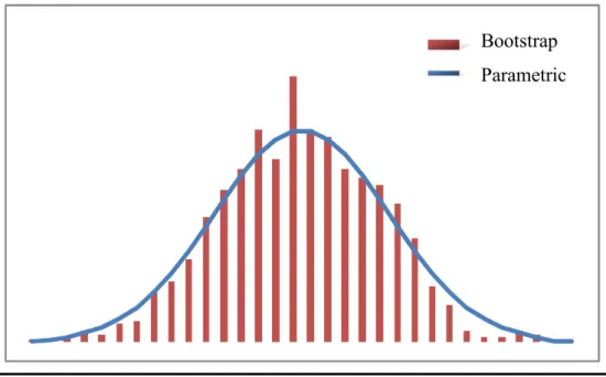
Figure 1: Comparison of Bootstrap and Parametric Sampling Distributions ... 51 Figure 2: Upper half bootstrap alpha histograms obtained using Henriksson and Merton Model ... 73 Figure 3: Histograms of the upper ranked alphas’ residuals obtained by
Henriksson and Merton timing model ... 74 Figure 4: Lower half bootstrap alpha histograms obtained using Henriksson and Merton Model ... 75 Figure 5: Histograms of the upper ranked alphas’ residuals obtained by
ix
Abbreviations
ISE Istanbul Stock Exchange
EFAMA European Fund and Asset Management Association USA United States of America
CAPM Capital Assets Pricing Model SMB Small Minus Big Sized Firms
HML High Minus Low Book-to-Market Equity Ratio Firms
PR1YR Difference of One Month Lagged 11 Month Return of Best and Worst %30 Firms’ Average Return
CMB Capital Markets Board of Turkey UK United Kingdom
ISE Istanbul Stock Exchange SML Security Market Line
ST1 Strateji Menkul De5erler A.E. A Tipi De5iIken Fon MAD Yatirim Menkul De5erler A.E. A Tipi De5iIken Fon NYSE New York Stock Exchange
BE/ME Book-to-Market Equity Ratio
KYD30 30 Days Bond Index of Turkish Institutional Investment Managers
1
1. Introduction
This study analyses the performance of 65 Turkish funds for the period February 2004 to December 2009 and tries to separate luck from skill using bootstrap procedure. Throughout the world there are various studies trying to measure the performance of mutual and pension funds. In these studies performance is decomposed into two components. One is called the timing component which is the ability of the fund manager to forecast the general behavior of the market prices and the other component is called the stock picking ability which is the ability of the manager to invest in exceptionally performing individual funds.
Jensen’s alpha is the most famous stock picking measure. Since the sixties, various regression models are developed for the appropriate alpha to measure the stock picking ability. Choosing the right model and discussing whether the fund managers have any stock picking ability is a popular topic held in detail. However, whether this alpha is due to true stock picking ability or chance is rather a new topic. It is first addressed by Kosowski, Timmermann, Wermers and White (2005) with the bootstrap methodology for US mutual funds and later by Cuthbertson, Nitzsche and O’Sullivan (2004) for UK equity mutual funds. According to our knowledge, this is the first study trying to separate luck from skill in Turkey.
By implementing bootstrap methodology for fund performance we try to improve the validity of the alpha measures. Historically well known performance measures have the assumption of normality for performance measure alpha meanwhile for a high percentage of funds in US and UK it is shown to be non-normal by Kosowski et al and Cuthbertson et al,
respectively. Varying risk levels of the funds also violates the assumption of normality for the joint distribution of the funds. For these purposes, we apply bootstrap procedure to the selected Turkish funds and try to create an environment where we can have an idea about the level of alphas that can be
2
achieved solely by chance. Then, we compare actual alphas with our bootstrap results and try to decide the level of stock picking ability for Turkish fund managers.
Funds that are included in this study are the ones that existed throughout the observation period. Excluding funds that do not satisfy this criterion may cause survivorship bias. To make sure the results that we obtain are valid, several survivorship bias measures are computed in light of the survivorship bias measure of Blake and Timmermann (1998).
This paper proceeds as follows: Section 2 gives a brief summary of the fund management environment and history for Turkish markets and the
comparison of it with the international ones. Then, the first four parts of section 3 discusses the literature of fund performance and presents the well known models of performance and the last two parts presents the resampling methodologies and several bootstrapping techniques. Section 4 presents our data and discusses the issue of survivorship bias which is a bias resulting from the exclusion of funds from the dataset. Further detail on the well known performance measures are given in section 5.1 together with the estimation results. Then resampling methodologies and bootstrap procedure is introduced and the reasoning behind using it is discussed in section 5.2. Empirical findings of the bootstrap procedure for several models are demonstrated in section 6. Finally section 7 concludes the study.
2. Developments in Mutual and Pension Fund Industry in
Turkey
Mutual fund is an investment product operated by professional managers that uses the money collected from many investors in return for participation certificates to invest in investment securities such as stocks, bonds, real estate, money market instruments, commodities, precious metals, other mutual funds and securities, with fiduciary ownership principals and
3
diversification of risk. Mutual funds are not legal entities, but to protect the rights of the investor the assets held within a mutual fund are separately held from the founder of the fund. Founder of the mutual fund is responsible for the protection and the safekeeping of the assets of the fund. Mutual funds are required to protect the assets under management by depositing them in a depository institution (the ISE Settlement and Custody Bank, Inc). This way it is ensured that the mutual fund assets aren’t affected from the state of the
founder, such as bankruptcy1. Moreover assets of a fund cannot be pledged,
used as collateral or seized by a third party, which fortifies the rights of the investor. Mutual funds in Turkey can be founded by banks, insurance companies, pension companies, intermediary institutions and eligible
retirement and provident funds2. They are managed by either intermediary
institutions or portfolio management companies with certain legal restrictions ensuring that the internal statute of the fund is met. There are certain limitations in the regulation of mutual funds in order to assure sufficient liquidity and proper diversification against risks taken. Mutual
funds can invest at most of their assets under management into the
securities issued by a single issuer. Mutual funds can invest in at most of any issuer’s total shares. Funds managed by the same manager can invest
in at most of any issuer’s shares in total. Mutual funds can invest at
most of their total shares into shares or dept instruments that are not
quoted to a stock exchange. Mutual funds can invest at most of their
assets under management into securities that are issued by the founder or the fund manager with the limitation that the amount invested in should at most
be of the issued security. Mutual funds cannot be represented in the
management of the companies whose shares it has purchased. Mutual funds
cannot short sell3. Mutual funds should maintain the fair price - buying from
the lowest possible price and selling from the highest possible price, in the transactions of the fund.
Turkish mutual funds are classified into two types which are called “Type
4
total holdings on monthly average basis into Turkish securities issued by Turkish companies. All other mutual funds are classified as Type B. Mutual funds are classified into different categories according to their
investment objectives. Funds that invest at least of their total assets for
all times in public and private debt instruments are called “bonds and bills
funds”. “Stock funds” are funds that invest at least of their assets
under management permanently in securities issued by Turkish companies.
“Sector funds” are the ones that invest at least of their assets
permanently in securities of companies belonging to the same sector. Funds
that invest of their assets under management for all times in securities
issued by subsidiaries are called “subsidiary funds”. “Group funds” are
funds that invest at least of their assets permanently in securities
issued by a certain group. “Foreign securities funds” invest at least of
their assets for all times in foreign public or corporate sector securities.
Funds that invest of their assets under management permanently in
gold and other precious metals or capital market instruments backed by these metals traded in national and international stock markets are called
“precious metals funds”. Funds that invest at least of their assets under
management for all times in gold and capital market instruments backed by gold in national and international exchanges are called “gold funds”.
“Composite funds” are funds that invest all their assets in at least two of the instruments like shares, dept instruments, gold and other precious metals or assets backed by them with the restriction that the share of each instrument
is not less than of the total fund assets. “Liquid funds” are funds that
invest all their assets continuously in liquid capital market instruments with less than 180 days to maturity with the requirement that the weighted average maturity of the portfolio being at most 45 days. Funds that cannot be classified in one of the above mentioned categories with respect to portfolio limitations are called “variable funds”. “Index funds” are funds
that invest at least of their assets continuously in an index or shares
5
the unit share value of the fund and the value of the index. “Funds of funds”
invest at least of their assets continuously in other funds. “Guaranteed
funds” are umbrella funds aiming a return over the total or part of the startup investment within a specified horizon with a guarantee of the guarantor and with an appropriate investment strategy. “Protected funds” are umbrella funds with the intension of a return over the total or part of the startup investment within a specified horizon with the best effort investment strategy. Finally funds with participation certificates given to certain
individuals or institutions are called “special funds’4.
Liberalization in Turkish economy began in early 1980’s. First move was the acceptance of the Capital Markets Law in 1981. Four years after the Capital Markets Law, in December 1985, Istanbul Stock Exchange was founded and began trading in 1986 in Ca5alo5lu office. One year later first communiqué regulating the mutual funds was formed and in July 1987, the first mutual fund was established by Ibank. This B type liquid fund is still alive. Also in 1987, Istanbul Stock Exchange moved to its modern
headquarters, which is the Karaköy office. In July 1992, new regulations consisting of the types of mutual funds were formed and A type funds were exempted from tax in order to encourage investments in stocks. Later on, extensive and innovative communiqué was launched in 1996 which is still in use. First private mutual fund, foreign mutual fund and sector fund were issued in 1997 followed by the issuance of the first index fund in 1999. In 2001 the first communiqué regulating the pension funds was published and in 2003 six pension fund companies started operating. In 2007 insurance law was published in the official gazette and with this law, several changes and extensions occurred in the communiqué regulating the pension funds. In order to secure the rights of the investors Pension Monitoring Center
controls the operation of the pension fund system. In 2007 the
responsibilities and authorities of the Pension Monitoring Center were redefined and several changes in the communiqué were made. Last revisions regarding the communiqué were made in 2008.
6
Some argue that the ancestors of modern funds were formed by a Dutch
merchant in late 18th century. Others argue that it was formed in 1882 by the
King of Netherlands. Although the roots are not certain first modern mutual fund was the Massachusetts Investors’ Trust which was established in 1924 and went public in 1928. Number of mutual funds is increasing since 1930’s especially escalating in 1980’s and 1990’s. The total mutual fund industry by the end of 2009 is 15.9 trillion euros. Out of this amount 55% is managed in Americas and 33% is managed in Europe. Largest single markets are USA, Luxemburg and France with investment assets amounting to 7.7 trillion euros, 1.6 trillion euros and 1.25 trillion euros, respectively. Turkey with investment assets of 13.4 billion euros has a market share of 0.085%. The most popular type of fund in both USA and Europe is the equity fund. Invested assets for equity funds are 3.4 trillion euros and 1.58 trillion euros, respectively. According to EFAMA statistics worldwide investment fund assets decompose as follows; 39% are invested in equity funds, 23% in money market funds, 20% in bond funds, 10% in balanced-mixed funds and 8% in other funds. By the end of 2009, there are 65306 mutual funds
operating worldwide. Out of these, 33054 is located in Europe, 286 of them being in Turkey, 16553 in Americas and 14795 in Asia and Pasific
countries.
Services provided by mutual funds cannot be limited to any timing or stock picking ability. Investing in mutual funds has certain advantages for small investors. First of all, mutual funds, manage huge amounts gathered by small investors. Thus, a mutual fund can easily invest in certain capital markets, derivative markets or international markets where small investors do not have access to. Further, due to the size of the total amount managed, or the bargaining skills of the professional managers hired, mutual funds can easily bargain and get better prices compared to small investors. Secondly, a mutual fund can keep more instruments in its portfolio compared to a small investor’s and hence provides diversification to the customers. In most
7
countries including Turkey, mutual funds are constructed as separate entities where any distress like default or bankruptcy of the parent company is isolated from the fund. Furthermore, the assets of the fund are kept in custody to ensure that mutual funds are legally safe investment alternatives. In addition to these advantages, mutual funds are supported by the
government where they are permanently exempted from the corporate tax. A mutual fund can also provide different strategy alternatives to small
investors where they cannot replicate, given the time and resource limitations. Index funds are example to strategies provided.
With all these advantages, mutual funds deduct management fees for the services provided, which is a negative effect compared to a similar portfolio constructed by the investor himself. Although the fund manager is not planning to change his position, due to incoming and outgoing cash flows, he might need to do trading, which creates transaction costs.
3. Review of Literature
Bootstrap is gaining more and more popularity in recent years due to
heterogeneous risk taking of fund managers and the non-normal distribution of individual fund alphas. Furthermore, bootstrap provides a powerful tool for performance persistence testing compared to parametric t-tests over past performance data. One of the most popular performance measures used in bootstrap procedures is the alpha.
3.1 Jensen’s Alpha and Other Popular Measures of 1960’s.
Alpha is the selectivity measure of Jensen (1967) which is the intercept of a one factor regression model, excess return of the fund regressed to the excess return of the market.
8
For time , is the return of portfolio , is the return of the market
portfolio and is the risk free rate. If the manager has any selection
ability independent from the state of the market, the regression line should shift upwards in parallel with any other ordinary portfolio manager. This upward shift causes the intercept (which was originally zero in the CAPM) to have a positive value which is represented by . One of the most important aspects of Jensen’s alpha is that it is an absolute measure rather than a ranking measure. Jensen has shown the bias of the least squares estimator . According to him, beta is downward biased proportional to the manager’s forecasting ability of the market. Hence if the manager doesn’t have any timing ability of the market, then will be unbiased and so will . But if the manager is capable of forecasting the market then will be downward and will be upward biased. But later Grant (1977) has shown that the bias caused by differs from Jensen’s both by magnitude and direction. Besides other advantages of investing in mutual funds (for example; diversification) Jensen investigated the stock picking ability. He examined 115 mutual funds for the period 1945 to 1964. He found very little evidence of stock picking ability. The results hold even for gross returns.
Treynor (1965) had developed a return over risk ranking measure. The most important aspect of the measure is how it defines the risk. Treynor assumes that risk component should not get affected from market fluctuations and should only reflect the variability of the fund compared to the market. So, the definition of risk for Treynor is the beta coefficient of the linear one factor regression of excess fund return over the excess market return.
(2)
Treynor measure gives an idea about the extra return gained against one unit of risk. One drawback compared to Jensen’s measure is that Treynor’s measure is a ranking measure rather than an absolute measure.
9
Sharpe compared to Treynor used the volatility of a fund as the measure of
risk and developed the “reward to variability ratio ”.
(3)
If the aim is to evaluate the past performance of a fund, the ratio will
be a better measure compared to Treynor ratio since, it includes the total variability. On the other hand, for predicting the future performance, Treynor ratio will be a better estimator since it is net of market variability and lets us identify the deviation from the market.
3.2 Performance Measures of Stock Picking Ability
Alpha is a measure of stock picking ability. But there are certain generally accepted trading strategies depending on firm characteristics which can beat the market but still, has nothing to do with any stock picking ability. For example one can beat the market with simply certain passive investment strategies like investing into high book-to-market equity ratio stocks. Fama and French (1993 and 1996) have investigated similar patterns and added them as independent variables to the factor model in order to purify alpha from this noise.
! " # $%&
! ' (%) *+
(4)
$%& (small minus big) is the index generated by Fama and French in order to capture the return of passive investment strategies related to size and (%) (high minus low) is the index used for strategies related to book-to-market equity ratio.
Jegadeesh and Titman (1993) documented that portfolios buying stocks with high past returns and selling stocks that have low past returns generate significant positive returns in the short run. Moreover, they have expressed that the significant returns deteriorates in three years time. Furthermore, Daniel, Grinblatt, Titman and Wermers’ (1997) findings suggest that there is a certain momentum effect in stock returns.
10
Affected by the work of Jegadeesh and Titman (1993) and Daniel et al (1997), Carhart (1997) developed Fama and French (1993 and 1996) model with a momentum factor.
! " # $%&
! ' (%) ! , - . *+
(5)
Along with size and book to market equity, - . , is the added factor
which is the one year momentum in stock returns.
Carhart, found that funds with good performance last year tend to have above average returns next year, but this above average return decays later on.
3.3 Performance Measures of Market Timing
Performance measures discussed previously were in search of stock picking ability. For the sake of a better measurement, they have tried to identify passive strategies which might affect alpha and added them as factors to the regression model. Besides stock picking ability, another important talent that the theoreticians tried to identify is the market timing ability. Market timing ability is the ability of the fund manager to identify the trends and update his position accordingly. Beta of a linear regression is the factor that measures the leverage of the market. So, if the manager has any timing ability he will decrease his beta in bad times and increase his beta in good times in order to optimize the effect of fluctuations of the market on his portfolio.
One of the well known efforts of market timing ability is the Treynor and Mazuy (1966) model. Treynor and Mazuy searched for any market
outguessing ability for 57 mutual funds during the period beginning in 1953 and ending in 1962. They defined the characteristic line as the fitted line between the market returns and the fund returns. Capital asset line is the sensitivity of the fund returns to the market returns. Assuming that the fund manager has any timing ability he will shift to less volatile securities (which means lower beta) if he anticipates that the market is going to fall and he
11
will shift to more volatile securities (which means higher beta) if he thinks that the market is going to rise. Since no manager claims to be able to predict the market perfectly Treynor and Mazuy assumes that the beta will increase as the market increases and decrease as the market decreases. High beta for good times and low beta for bad times condition in practice occurs as a beta smoothly increasing or decreasing according to market conditions rather than two lines with an elbow, which means a concave upwards capital asset line. To capture this convexity, Treynor and Mazuy added the square of the excess market return to the regression.
/ # *+ (6)
/ captures the timing ability of the manager. They empirically found that there is only one fund with market timing ability which can be explained by luck so; there is no evidence of market timing ability. Hence, portfolio managers shouldn’t try to time the market.
Henriksson and Merton (1981) assumes that the manager can only forecast whether the market return exceeds risk free rate or not and doesn’t have any information of the magnitude of it. So instead of squared market excess return as in Treynor and Mazuy (1966), they used a dummy variable 0 indicating the two states of the world.
/ 1 02 *+ (7)
0 3 4
5 6
(8)
A statistically significant and positive / will mean that the portfolio
manager has market timing ability.
3.4 Conditional Performance Measures
Until now we have discussed unconditional models of performance. But in reality, alpha and beta values may be conditional on a specific information set and they may be time varying. Thus, in a world where the alpha or the
12
beta is conditional on any information set, measuring performance over unconditional averages will give us to misleading results.
Ferson and Schadt (1996) have conditioned the beta to certain market
information. They have assumed that beta, 7 8 consists of two
components: the average long term beta, 9 and beta conditioned on market
information, : .
7 8 9 : ; (9)
Here, ; is the vector of the deviations from the expectations of the information 8 that the beta is conditioned on. The conditional beta definition of Ferson and Schadt can be implemented into any regression model. For example the conditional form of eq. (1) will be as follows:
< =" ! 9 <7 =" : ; <7 =" * =" (10)
where < =" =" =" and <7 =" =" =". Ferson and
Schadt showed empirically that conditioning the performance measures is statistically significant. They have also concluded that the inferior alpha performance is due to using unconditional average information and the distribution of alpha shifts through zero after conditioning the beta to market information. Furthermore, they have also expressed conditional versions of Treynor and Mazuy (1966) and Henriksson and Merton (1981) better predict market timing ability.
Christopherson, Ferson and Glassman (1998) have further developed the conditional model of Ferson and Schadt with conditioning the alpha as well as beta.
< =" ! 9 > ; 9 <7 =" : ; <7 =" * =" (11)
Where 9 is the average alpha and > is the alpha that is time varying,
conditioned on the information set 8 . They have analyzed pension fund data and found that bad performance persists.
13
3.5 Bootstrap and Other Resampling Approaches
Bootstrap is a simulation based statistical analysis which is an alternative to the traditional statistical techniques that assume certain probability
distribution. It is a process of resampling the data at hand to build a sampling distribution. The research on this topic began in the late 1970s although early work that influenced bootstrapping traces back to 1920s to R. A. Fisher’s work on maximum likelihood estimation (Efron, 1998). Fisher’s method is not only practical but also looses less information in small
samples. Smart mathematics he uses was an advantage before the
technological developments, now bootstrap has the advantage in this sense. The similarity of Fisher information with bootstrap is the substitution of the estimates for the unknown parameter. There are also other methods,
resampling methods that are related to the history of bootstrapping such as jackknifing, cross-validation, random subsampling and permutation tests. Jackknife was first introduced by Quenouille (1949). Jackknife statistics are produced by dropping out data from the sample one at a time and
calculating the necessary statistics over that new sample. This technique lost its popularity to bootstrapping, since it is more generalized, but jackknife is easier to apply to complex sampling.
Cross-validation is another resampling method that predates bootstrapping. “Leave one out” cross-validation is usually confused with jackknifing. Both techniques omit one observation at a time and work on the remaining subset. But while jackknifing is used to estimate the bias of a statistic,
cross-validation is used to estimate the prediction error. Cross-cross-validation is a way of measuring the prediction accuracy of different models and selecting the one with the smallest prediction error. K-fold cross-validation is done simply by dividing the observation set into k equal (or near equal) segments, leaving one segment for testing and working with the other k-1 segments for building the model. Bootstrapping has small variance in small samples while cross-validation nearly provides unbiased estimates of prediction
14
error. A type of bootstrapping (.632+ bootstrap) outperforms
cross-validation according to Efron and Tibshirani (1995). Random subsampling validation is done by choosing repeated random sets for validation and training. This repeated randomness causes some observations to appear more than once and some not at all in the validation set which biases the results.
Another resampling method used in the literature is the permutation test which is based on the work of R.A. Fisher in the 1930s. It checks the significance of a statistic by forming a distribution of it from all possible rearrangements of the sample. It is commonly used for testing whether the distributions of two samples are equal, while bootstrapping is used for parameter estimation. Because of this specific hypothesis, permutation test has a limited use. Compared with the parametric methods, both permutation test and bootstrapping have the advantage of finding results without making parametric assumptions. But when applicable, permutation test gives exact results while bootstrapping gives only an approximation.
Most of the developments on the bootstrap theory occurred after Efron (1979). Eventhough this new technique didn’t grab researchers’ attention at first, Efron’s continuous publications on the topic created the deserved curiosity. Bickley and Freedman (1981) and Singh (1981) tested the accuracy of the technique on several ocations and showed that the
bootstrapping works for the sample mean when there are finite second order moments. Bickley and Freedman (1981) also gave some examples for situations where bootstrapping failed. There are many other research papers about the consistency of bootstrap technique (such as Athreya (1987) and Gine and Zinn (1989)) but there is still a lot to search, especially for the complex samples. There were alot of suspicions regarding the bootstrap methodology at first. The work of Efron and Tibshirani (1986) was a somewhat successful attempt to clarify the minds of scientists, but as Chernick (1999) explains in his book, oversimplicity of the expressions and
15
the lack of mathematical theory resulted misunderstandings about the methodology.
After asymptotic consistency of bootstrapping became a popular research topic, the limitations and possible applications of it became clearer.
Researches realized that bootstrapping isn’t only used for estimation of the standard errors, confidence intervals and hypothesis tests but it can be used for a wide class of problems such as regression problems, time series analysis and density estimation as well as a wide class of fields such as geology, medicine, engineering, biology, psychology and econometrics. Having no assumptions about the distribution of the sample not only made bootstrapping applicable to many situations but also made things a lot easier. The simplicity of the technique made it more attractive among scientists, especially with the growing developments on computer
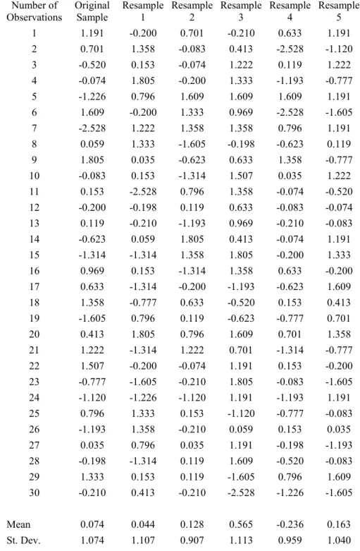
technology. The idea with basic bootstrap is always to construct a sample with replacement from the original sample, compute the necessary statistics for the bootstrapped sample, repeat these steps many many times and obtain a distribution of the bootstrap statistics. You can then compare your results with the original statistics. The important thing is to be careful about the limitations of bootstrap and avoid using it when there is evidence of theoretical drawback. It is believed that bootstrapping gives acceptable results when all other approaches are eliminated with the assumptions of the sample.
There are various types of bootstrapping some of which are basic non-parametric bootstrap, non-parametric bootstrap, smooth bootstrap and moving block bootstrap. The basic bootstrap technique makes no assumptions about the population distribution and assumes that the sample at hand is a good representative of the population and drives conclutions using the sample. Therefore it is actually a non-parametric technique. If there is an assumed parametric distribution for the population, the estimate of interest can be calculated using parametric bootstrap method. In parametric bootstrap,
16
samples are drawn from the parametric estimate of the population rather than using resampling with replacement from the sample. Other than this, the procedure proceeds similar to basic bootstrap. For each bootstrap iteration the relavent statistic is calculated and using these values bootstrap distribution is obtained. According to Efron and Tibshirani (1993),
parametric bootstrap gives more accurate answers than analytic formulas and in the state of lacking these formulas it can provide answers. It is useful when some information about the population is available. It helps to deduce conclusions without any use of complicated formulas. It is not very common to use parametric bootstrap since the distribution of the population is known but some statistics are not easy to calculate and parametric bootstrap saves us from the trouble.
Smoothed bootstrap like parametric bootstrap doesn’t use sampling with replacement from the sample. It rather uses sampling from a smooth estimate of the population. Efron (1982) applied smoothed bootstrap to estimate the standard error of the correlation coefficient using both Gaussian and uniform kernel functions and the results indicated that smoothed
bootstrap estimations were somewhat better than the basic non-parametric bootstrap results. Silverman and Young (1987) found some conditions to use smoothed bootstrap procedure.
Basic non-parametric bootstrap method assumes that the observations are independent but this may not be the case for time series data or other correlated data. Moving block bootstrap is applied to correlated data. The sample is divided into ? nonoverlapping blocks of @ consecutive
observations such that ?@ gives approximately the sample size. Bootstrap sample is constructed by randomly sampling ? blocks with replacement and linking them together. This method is used to preserve the correlation within the data. The correlation between the observations is assumed to be
strongest within the blocks and weaker between them. So the size of the blocks, @ is important. If @ is large, then the number of blocks (?) is small so
17
the bootstrap samples will mostly be the same. If @!is small, then
observations in different blocks may not be independent which will reduce the accuracy of the inferences (blocks are assumed to be independent while bootstrapping). @ should be choosen so that the observations that are @ units apart from each other are nearly independent. This way the correlation present within a block is preserved. Moving block bootstrap is introduced by Carlstein (1986) and Künsch (1989) and then discussed by Efron and Tibshirani (1993). If the block length is choosen correctly it provides a simple alternative to parametric time series models preserving the empirical distribution and the correlation of the original sample.
Another application field of bootstrapping is the regression models. Regression models are useful tools in sorting out the effects of certain explanatory variables on a response variable. Ordinary least squares (OLS) estimation technique is commonly used for estimating the coefficients of the explanatory variables. But it is a good proxy only if the underlying
assumptions are satisfied. Especially in small samples, the extreme values may cause the normality assumption of the residuals to be violated. The residuals may also have heavy-tailed distributions rather than normal. Both these factors cause least squares estimation to be misleading. Bootstrap procedure helps to manage these problems. Efron (1982) introduced two possible procedures for regression models, one of which is bootstrapping the pairs. With this procedure the explanatory variables of the regression model are treated as random. Vectors of the response variables with the
corresponding explanatory variables are constructed and the resampling methodology is applied to these vectors with replacement. These vectors are then used to fit the model and obtain bootstrapped regression coefficients. The estimated bootstrap distribution of each regression coefficient is formed using equal probability.
The other bootstrap procedure that Efron (1982) proposed is called
18
fixed and uses the residuals instead. It is more complex compared to basic non-parametric bootstrapping since an underlying model should be
structured in order to obtain the residuals. So the first step is to fit a model to the sample and obtain the observed residuals by simply subtracting the multiplication of the explanatory variables with the estimated coefficients from the response variable. After this procedure, for each bootstrap replication resample the residuals with replacement and adding these bootstrapped residuals to the multiplication of the explanatory variables with the estimated coefficients, obtain the bootstrapped response variables. Then regressing bootstrapped response variables against the explanatory variables, estimate the bootstrapped regression coefficients. As always these coefficients are used to form bootstrap distributions of the regression
coefficients.
Since bootstrapping the residuals preserve the information coming from the explanatory variables, the choice of the model gains importance. If the underlying regression model isn’t the best choice, bootstrapping the residuals may give misleading results. Efron claims that bootstrapping the pairs is less sensitive to this kind of faulty model selections. Therefore if there are doubts about the choice of the underlying model, it is better to use bootstrapping the pairs approach. Efron and Tibshirani (1986) assert that the results obtained from bootstrapping the pairs approach approximates to the results obtained from bootstrapping the residuals approach. But these methods differ for small samples therefore one should be careful dealing with them. Bootstrapping doesn’t have strict boundaries. In some instances, even though the explanatory variables are random, it may be best to use bootstrapping the residuals approach and act as if they are fixed. The underlying model doesn’t have to be a perfect fit for bootstrapping the residuals to give acceptable results.
The next section deals with two applications of bootstrapping the residuals approach used for fund performance.
19
3.6 Applications of Bootstrap Method to Fund Performance
Kosowski, Timmermann, Wermers and White (2005) tried to distinguish luck and skill in the performance measure of alpha. The pioneering work of Kosowski et al is the first paper that uses bootstrap technique for this purpose. Furthermore, they try to reconstruct data by bootstrapping to test for persistency rather than analyzing past performance results to forecast future performance. Bootstrap technique has some certain advantages. Most importantly, as the distribution of the alphas is complex and non-normal, bootstrap is very convenient to use in the sense that it doesn’t require any distribution to be defined. Kosowski et al applied bootstrap techniques to the conditional (as defined by Ferson and Schadt (1996)) and unconditional versions of Carhart’s four factor model over the period of 1975 to 2002 on monthly net returns of US open-end domestic equity funds. Although there is certain amount of luck, there is also superior performance, especially in
the top of the funds. Another result of the bootstrap tests is that
superior fund performance exists for growth oriented funds which is a result first given by Chen, Jegadeesh and Wermers (2000).They also stated that there is no superior fund management ability in income oriented funds. Although there are variations in ability for high alpha funds due to stock picking ability, the differences in low ranked funds are due to expenses rather than skill. Kosowski et al made some checks to assess whether the time series dependence of the residuals have a bad effect on their results. In unreported tests they found that the results are almost identical to their findings with bootstrapping the residuals approach. They also checked whether a possible correlation between the explanatory variables and the residuals have any effect on their results by resampling both the explanatory variables and the residuals. Again they found almost identical results. They finally tested the effect of cross-correlation between fund residuals and found almost identical results. These results suggest that using
bootstrapping the residuals approach is a good and simple choice of finding the approximatted distribution of the parameters.
20
Cuthbertson, Nitzsche and O’Sullivan (2004) applied bootstrap techniques following Kosowski et al (2005) to the largest European mutual fund market, UK. They used 1596 open end mutual funds for the period of April 1975 to December 2002 from which 450 of them are non-surviving to overcome the survivorship bias. They used funds with at least sixty
observations to overcome any possible sampling bias. They have classified funds according to their objectives and searched whether outlier
performances are based on skill or luck. Cuthbertson et al applied CAPM, multi-factor models of Fama and French (1996) and Carhart (1997), market-timing models of Treynor and Mazuy (1966) and Henriksson and Merton (1981). They have also conditioned these five models following Ferson and Schadt (1996), which conditions only beta to available market information and also Christopherson, Ferson and Glassman (1998), which conditions both alpha and beta to available market information resulting 15 different performance measures of alpha. They have shown that conditioning the models or adding a market timing term do not improve the measure and that the best fit model is the unconditional Fama and French model. Similar to Kosowski et al, Cuthbertson, Nitzsche and O’Sullivan found that there is stock picking ability in best performing funds which cannot be related to chance by itself and that relation is even stronger for worst performing funds. They have measured the performance over the defined classes according to investment objectives and contrary to Kosowski et al, who found stock picking ability for growth oriented funds, they have found strong stock picking ability both for income and growth oriented funds for UK.
4. Data
This study examines monthly returns of 46 mutual funds and 19 pension funds, a total of 65 funds for the period in between January 2004 and December 2009 (their codes and names are available on Appendix A). Mutual funds that are included in this study are A-type, which means at
21
least of the funds for all times are invested in securities issued by
Turkish companies. On the other hand pension funds that are included
contain at least of their shares as stocks. According to the
classification of the Capital Markets Board of Turkey (CMB), 10 of the pension funds that are included in this study are growth oriented, 1 of them is income oriented and 8 of them are classified as “other”. The dataset is obtained from the monthly bulletins of CMB and several corrections are made which are listed in Appendix B.
Pension funds that invest in foreign securities are excluded from the sample, since the benchmark that we use for funds that invest in Turkish securities will not give appropriate results for funds that invest in foreign securities. Similarly, mutual funds with an investment objective of foreign securities are excluded. Moreover, mutual funds that invest in ISE indices are excluded as well, since they are overly correlated with the benchmark and their objective is market tracking (which means they are not trying to outperform the market and so it’s not reasonable to search for performance for these types of funds).
There are 139 funds that meet the above criteria, but are excluded from the sample. There are possible reasons for this exclusion: Funds may merge, the investment companies may go bankrupt, funds may disappear because of poor performance during the observation period or funds may be established during the observation period, which in most cases means they don’t have enough observation. The funds are chosen with the condition that they were born before the observation period and survived until the end of December 2009. This may cause survivorship bias, because the funds that terminated during the observation period are not included. The funds that couldn’t survive until the end of the sample period are the ones which are expected to have poor performance. Excluding these funds from the sample period may cause the performance measure, alpha to be over estimated. The effect of non survivng funds, was analyzed by Blake and Timmermann (1998). They
22
analyzed 2300 UK open-ended mutual funds between February 1972 and June 1995 with the following formula:
?ABC D<CE E
FFE E<FE E FCE E <CE E FFE E FCE E G
(12)
where FFE E is the number of non-surviving funds for month , FHE E is the
number of surviving funds for month , <IE E is the equally weighted
portfolio return of non-surviving funds for month and <HE E is the equally
weighted portfolio return of surviving funds for month .
They have found a considerable amount of survivor bias of J per annum
for UK constructing two portfolios for funds that died during the
observation period and for funds surviving until the end of the period. They have further investigated the fund behaviors before termination and after birth and found significant underperformance prior to termination, but slightly over performance in the early periods after birth. They have constructed a zero cost portfolios of best and worst performing funds, monthly rebalanced depending on the past 24 months’ average performance and found significant persistence on both sides.
To check whether this bias has an important role for our sample period, survivorship bias measure of Blake and Timmermann (1998) is computed. For the sample period we examine, there are 80 non surviving funds in total
and 65 surviving funds that we choose. J K !monthly bias corresponds
to J L annual bias for our sample period, which at first seems like a
similar result for UK, but considering the volatility of Turkish markets, it is less important.
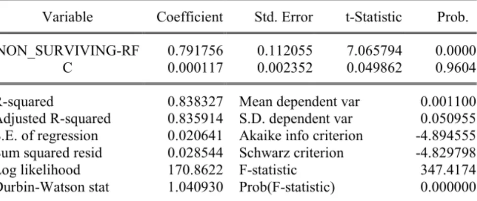
Moreover we examined survivorship bias by regressing the surviving funds’ monthly average excess returns on non-surviving funds’ monthly average excess returns with the null hypothesis that alpha is zero.
23
This way, if there is any extra performance (which corresponds to a positive and significant alpha) we may conclude that there is survivorship bias for our sample period. From Table (1) we can check that the intercept, alpha is
J (which is minor) with the probability! J L. Hence we cannot reject
the null hypothesis and we may conclude that our data contains no
survivorship bias. Further studies on survivorship bias for Turkish markets are examined at Appendix C.
Table 1: Regression results of surviving funds on
non-surviving funds5
Dependent Variable: SURVIVING-RF Method: Least Squares
Sample (adjusted): 2004M02 2009M10 Included observations: 69 after adjustments
Newey-West HAC Standard Errors & Covariance (lag truncation=3)
Variable Coefficient Std. Error t-Statistic Prob.
NON_SURVIVING-RF 0.791756 0.112055 7.065794 0.0000
C 0.000117 0.002352 0.049862 0.9604
R-squared 0.838327 Mean dependent var 0.001100
Adjusted R-squared 0.835914 S.D. dependent var 0.050955 S.E. of regression 0.020641 Akaike info criterion -4.894555 Sum squared resid 0.028544 Schwarz criterion -4.829798
Log likelihood 170.8622 F-statistic 347.4174
Durbin-Watson stat 1.040930 Prob(F-statistic) 0.000000
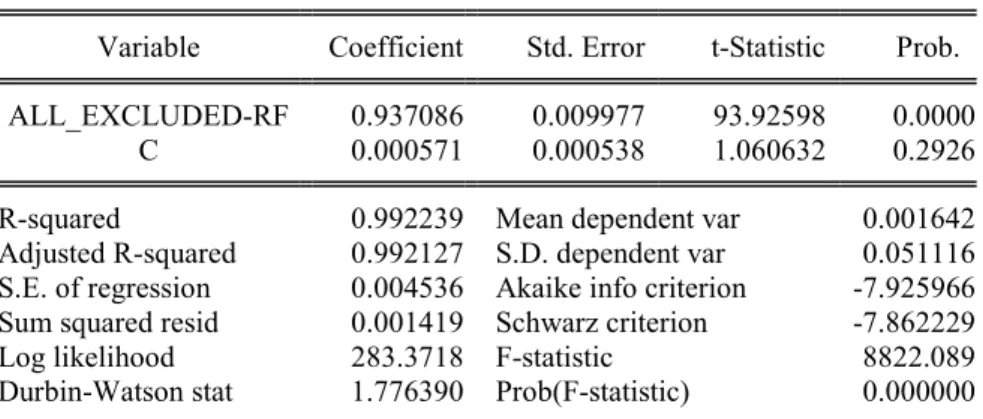
There is one more bias that we should consider. Our data set consists of funds which have full data during our sample period, but there are 59 funds that were established during the sample period as well as 80 non-surviving funds that we don’t take into account. Not analyzing these 139 funds may cause “exclusion bias” to occur. Regenerating the above regression for monthly excess average returns of included funds and excluded funds gives
24
null hypothesis of zero alpha. Reconstructing Blake and Timmermann (1998)’s measure for exclusion bias gives us the below equation
OPQJ ?ABC D<CE E
F*E E <*E E FCE E<CE E F*E E FCE E G
(14)
where, FRE E represents the number of excluded funds for month and <RE E
is the equally weighted portfolio return of excluded funds for month . Our
results suggest a JS per annum bias which is negligible.
Table 2: Regression results of included funds on excluded funds
Dependent Variable: SURVIVING-RF Method: Least Squares
Sample: 2004M02 2009M12 Included observations: 71
Variable Coefficient Std. Error t-Statistic Prob.
ALL_EXCLUDED-RF 0.937086 0.009977 93.92598 0.0000
C 0.000571 0.000538 1.060632 0.2926
R-squared 0.992239 Mean dependent var 0.001642
Adjusted R-squared 0.992127 S.D. dependent var 0.051116 S.E. of regression 0.004536 Akaike info criterion -7.925966 Sum squared resid 0.001419 Schwarz criterion -7.862229
Log likelihood 283.3718 F-statistic 8822.089
Durbin-Watson stat 1.776390 Prob(F-statistic) 0.000000
As a result, our findings suggest a minor bias caused by not taking into account all the funds existing during the period of January 2004 to December 2009. Therefore we may conveniently use the results obtained from the data set.
The benchmark that is used throughout the paper is ISE100 index issued by Istanbul Stock Exchange. Risk free rate is taken to be the 30 days bond index issued by Turkish Institutional Investment Managers Association. Monthly return data is used for fund evaluation. Returns are computed
25
simply as the difference of the price change from prior month to the next one, divided by the price of the prior month.
- - T"
- T"
(15) Where - is the price of the fund at the end of the month . Prices are published in the monthly bulletin of the Capital Markets Board of Turkey at the end of the month. These prices are announced after deduction of fees and expenses.
5. Methodology
Bootstrap procedure is gaining importance in the literature of fund performance for several reasons. Investigations suggest that varying risk levels of the managers and the non-normalities of the individual fund alphas cause cross section of alpha measures to be non-normal. This contradicts the assumption of normality that many of the performance models used before for checking the statistical validity of the measures. In order to resolve this problem bootstrap technique is used which doesn’t impose a distribution for fund performance and allows us to construct a sampling distribution of fund performance. First, we will discuss the generally accepted performance models and apply them to our data set in order to choose the most
appropriate models to use in our bootstrap simulations. Then we will argue the advantages of bootstrapping procedure and define the process.
5.1 Regression Models Used
In this section, commonly used performance measures are discussed and appropriate models are selected for intensive bootstrap procedure for Turkish funds. After examining unconditional performance models of Jensen, Fama and French, Carhart, Treynor and Mazuy and Henriksson and Merton for the dataset, we will give beta and alpha and beta conditional results of specific models on Ferson and Schadt and Christopherson, Ferson and Glassman sense, respectively. Since bootstrapping is an intensive
26
process, we will choose best explaining model for each of the three
categories (unconditional, conditional on beta and conditional on alpha and beta) and discuss the results. For brevity, reports will be given as the
averages of the values estimated. All t statistics are reported as the averages of the absolute values of the t statistics to prevent negative and positive values to cancel each other out, except for the t statistics of the equally weighted portfolios constructed.
5.1.1 Jensen’s One Factor Model
The most known performance measure is Jensen’s single factor model, which is given by eq. (1). The only risk factor represented in this model is the market. If CAPM is the correct model of equilibrium returns, then the portfolio should be on the Security Market Line (SML), which indicates that the intercept alpha of the regression model should be zero. This implies that, a positive and significant alpha from the regression is the extra performance of the portfolio manager over the market. Jensen claims that if the portfolio manager has some stock picking ability, he will continuously perform better
than the market providing this positive alpha. The risk free rate !used for
Turkish funds as discussed before is the monthly return of the 30 days bond index issued by Turkish Institutional Investment Manager’s Association at the end of month! .
U
-VWX'9E -VWX'9E T" -VWX'9E T"
(16)
The proxy of the market portfolio which is represented by , is the
monthly return of the ISE100 index issued by Istanbul Stock Exchange at the end of month! .
The results of CAPM regression model is presented at the first column of table (3). Average of the alpha estimates of 65 Turkish funds that we
consider is J per month which corresponds to JLY annually.
This indicates that on average mutual fund managers underperformed the
27
this abnormal performance is insignificant. Although not reported this
model gives significant results for only L of the funds and alpha
performance varies in between the values JS and JKY with the best
performing fund being ST1 and the worst performing fund being MAD. Models considered after CAPM are more extensive and therefore we expect them to give better estimates of performance.
5.1.2 Treynor and Mazuy’s Market Timing Model
Treynor and Mazuy (1966) studied whether portfolio managers try to outguess the market movements and replace their beta, the sensitivity of their portfolio to the market, accordingly. Their assumption of increasing beta as the market moves upwards and decreasing beta as the market moves downwards rejects constant beta. Hence they define beta as a linear function of the market factor, replace it in CAPM regression model and obtain eq. (6).
The results of Treynor and Mazuy timing model are presented in column 3
of table (3). Our regression results on average give J monthly
performance but as CAPM model this performance is not significant at 5%. Negative performance switches to positive performance with Treynor and Mazuy timing model indicating that managers have stock picking ability.
Between JSK and J L monthly alpha performance results with only
9% of these performances being significant at 5%. Similar to CAPM model, ST1 is the best and MAD is the worst performing fund. The market timing
component on average is Y JL which indicates that Turkish funds
cannot time the market although they have stock picking ability. 49% of the funds considered have significant market timing component with 5% significance level. These results indicate that the reason for negative performance coming from CAPM measure is the lack of the timing component. Treynor and Mazuy model corrects this problem.
28
5.1.3 Henriksson and Merton’s Market Timing Model
A similar market timing model is constructed by Henriksson and Merton (1981). They suppose that the manager forecasts whether the market exceeds the risk free rate or not, but don’t take in to account the magnitude of it. The manager will have a higher beta if he has a positive forecast and lower beta otherwise. They construct beta as a function of a constant term and a dummy variable (eq. (8)) which gives 1 for positive market forecasts and 0 otherwise. Similar to Treynor and Mazuy, they replace this beta in CAPM regression model and obtain eq. (7).
The results of the Henriksson and Merton timing model are presented in the
second column of table (3). We obtain JL monthly performance on
average but this value is insignificant at . This alpha performance is
better compared to the alpha obtained from Treynor and Mazuy timing
model, but still for only K of the funds we have significant alphas. The
best fund is ST1and it has SJ monthly performance with the model and
the worst one is MAD with a JK monthly performance. The negative
coefficient of the dummy variable which is the measure of market timing indicates that Turkish funds on average have negative market timing ability.
Y of the funds have significant coefficients of market timing at
significance level. This result is similar to the result obtained from Treynor and Mazuy timing model.
5.1.4 Fama and French’s 3 Factor Model
Fama and French (1993), reports that funds may have investment strategies related to firm characteristics and these should be added to the model as explanatory variables in order to rectify alpha from their misleading effects. They improve Jensen’s one factor model, CAPM by adding two additional factors, $%& and (%). $%& stands for “small minus big” index which is a proxy for the size effect and (%) stands for “high minus low” index which is a proxy for the effects related to the book-to-market equity ratio. For the calculation of these indices, Fama and French first find the median of the
29
market equities of the NYSE securities and separate them into two classes as “small” and “big”, $ and &, respectively. Market equity for a fund at time
is calculated as the product of the price and the number of shares at that period. They then divide these securities into three different groups relative
to their book-to-market equity ratios &O %O in a way that the highest
S of these securities are in the “high” group, (, the lowest S of them
are in the “low” group, ) and the middle Y are in the “middle” group. %.
They calculate the book equity &O as the book value of the equity plus the
deferred taxes and the investment tax credit, minus the book value of the
preferred stocks6. Then &O %O is simply &O at the fiscal year ending of
calendar year divided by %O at the end of December of year . If
the firms have negative book-to-market equity ratios, they are excluded from the sample of observations. Fama and French (1992a) in their paper found that book-to-market equity ratio proxy better explains the returns then size proxy, which is why the securities are classified into three groups relative to their book-to-market equities and two groups relative to their sizes. Using these groups, the following six portfolios are formed $ (E $ %E $ )E & (E & %!and & ). If a stock is small sized and it has high book-to-market equity ratio for a given time period, then it will be in portfolio $ (. Even though &O %O and &O are calculated at the end of the year
, these portfolios are formed six month lagged at the end of June of year , which is realistic considering the fact that some time will pass until the investors obtain these figures. For each portfolio, returns are weighted according to their market equities. Then, $%& and (%) are formed accordingly;
$%& $ ) $ % $ (
S
& ) & % & ( S
(17)
(%) $ ( & ( $ ) & ) (18)
We adapt Fama and French’s formulation while calculating $%& and (%), but we use publicly available book-to-market equity and market equity values for each year end from the website of ISE. Similarly, price data for
30
month ends of every stock trading in ISE are gathered from the website of ISE in order to calculate the monthly returns of the stocks.
Using eq. (4), we regress the 65 funds that we choose and obtain J
monthly performance on average. This negative performance isn’t
significant at level. The best and the worst performing funds are ST1
and MAD having J Y and JL , respectively. Alpha coefficients are
significant for S of the funds. Compared to CAPM, there is a slight
increase in performance. This is the effect of the factors added. The
coefficient of $%& is positive (SJLY ) and significant for SK of the funds
where as the coefficient of (%) is negative ( YJ ) and significant for
L of the funds. These positive and negative coefficients imply that managers in Turkey prefer small sized stocks with low book to market equities.
5.1.5 Carhart’s 4 Factor Model
Carhart’s four factor model is an extension of Fama and French’s three factor model. Reports of Jagadeesh and Titman (1993) that portfolios buying winning stocks and selling looser stocks return positive earnings in the short run imply the presence of momentum effect. We should keep in mind that return gained by using this zero investment strategy, which is publicly available, isn’t an extra performance generated by the portfolio manager. In order to capture this momentum effect, Carhart uses an additional risk factor, one year momentum proxy to measure manager’s performance. For Carhart’s model, the proxy of one year momentum effect,
- . is the return difference between a portfolio with previously high
performing stocks and a portfolio with previously low performing stocks. To construct these two portfolios, we first form prior 11 month returns of all the stocks available with the following formulation;
EZ[\][ ^_M E TI N
""
I`"
a
31
where E TI !is the return of the stock at time! F.Then we rank the
stocks using their prior 11 month returns, EZ[\][ and form two portfolios
using simple average returns of the highest S of the funds and the lowest
S of the funds. Adding this new proxy to Fama and French’s three factor
model, Carhart’s four factor model becomes as in eq. (5).
As can be seen from the fifth column of table (3), our regression results
suggest J monthly average performance which is the same value
obtained from Fama and French’s three factor model. This performance is
insignificant at level. The alpha performance measure varies between
J and JL and S of these performances are significant. Similar
to Fama and French’s model, $%& has positive and (%) has negative
effect. The negative coefficient of the new factor - . is insignificant on
average. Actually this coefficient is significant for only of the funds, which is minor. Further comparisons between the models discussed will be given later for model selection for bootstrap analysis.
32
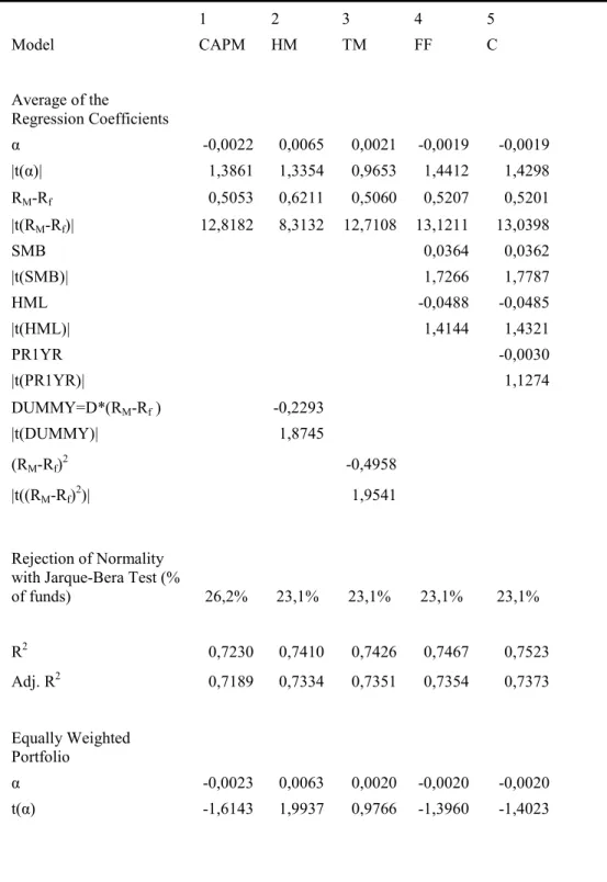
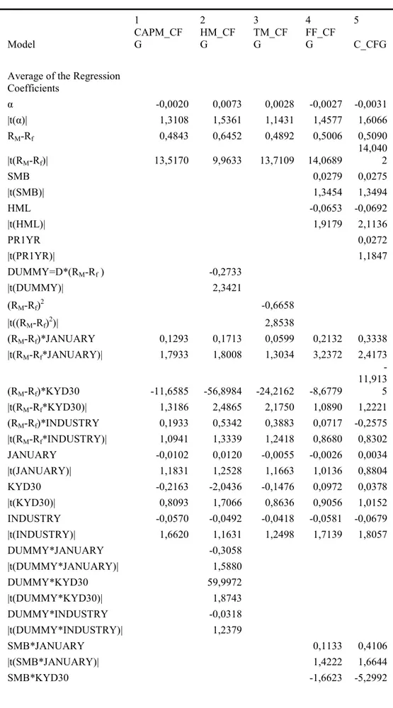
Table 3: Regression Results of the Unconditional Models
1 2 3 4 5 Model CAPM HM TM FF C Average of the Regression Coefficients ^ -0,0022 0,0065 0,0021 -0,0019 -0,0019 |t(^)| 1,3861 1,3354 0,9653 1,4412 1,4298 RM-Rf 0,5053 0,6211 0,5060 0,5207 0,5201 |t(RM-Rf)| 12,8182 8,3132 12,7108 13,1211 13,0398 SMB 0,0364 0,0362 |t(SMB)| 1,7266 1,7787 HML -0,0488 -0,0485 |t(HML)| 1,4144 1,4321 PR1YR -0,0030 |t(PR1YR)| 1,1274 DUMMY=D*(RM-Rf ) -0,2293 |t(DUMMY)| 1,8745 (RM-Rf)2 -0,4958 |t((RM-Rf)2)| 1,9541 Rejection of Normality with Jarque-Bera Test (%
of funds) 26,2% 23,1% 23,1% 23,1% 23,1% R2 0,7230 0,7410 0,7426 0,7467 0,7523 Adj. R2 0,7189 0,7334 0,7351 0,7354 0,7373 Equally Weighted Portfolio ^ -0,0023 0,0063 0,0020 -0,0020 -0,0020 t(^) -1,6143 1,9937 0,9766 -1,3960 -1,4023
33
5.1.6 Ferson and Schadt Conditional Model
The measures discussed until now are unconditional models of performance, i.e., they don’t take into account the changing information about the market. If the portfolio manager changes his portfolio composition and risk in accordance with the changing information about the expected returns and risk of the securities contained in the portfolio, the unconditional measures of performance will give biased results. There are possible reasons for the risk of the portfolios to shift through time: Market corrects the over pricing or the under pricing of securities and companies change their financial strategies. Hence even if the manager follows a buy and hold policy, the risk of the portfolio changes over time because of the risk changes of the
underlying securities and the weights of these securities change as well in accordance with their values. Moreover, actively managed portfolios betas and weights will change continuously. To purify the performance measure alpha from the effects of these risk shifts Ferson and Schadt (1997)
conditioned their beta to a publicly available information set. Their intuition is that if the manager uses publicly available information, it shouldn’t be judged as superior performance and should be eliminated from the
performance measure alpha. Eq. (10) gives the beta conditional regression model of CAPM. We may generalize this equation for multiple factor regression models by simply conditioning the betas of the risk factors to the publicly available information set!8 .
< =" ! b \ c\ ="
V
\`"
* ="J (20)
If we have a d factor regression model with c\ =" defined as the i-th risk
factor’s portfolio at time , \ as the beta coefficient corresponding to
this portfolio and < =" as the excess return of fund at that time period
( =" ="), we may convert this unconditional model to a conditional model by replacing the beta coefficients of the risk factors with a linear function of them as defined earlier by eq. (9).