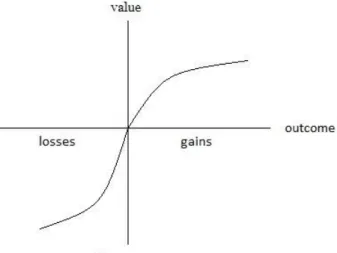
A credit design for irrationally pessimist entrepreneurs

For a given target photo and set of initial tags, the method retrieves relevant photos and their corresponding tags from Flickr (Step 1); forms a candidate tag list by

When the features of the bonds are not constant over time, our implied default probabilities may be an improvement over the yield and/or price as a measure of credit quality, in

triplicate samples treated with different stimulants (PS1-4, PGN and LPS).. Although previously PS2 activity in culture was similar to PS4, surprisingly it failed to reproduce

At high frequencies the sample does not have enough time to charge nor discharge resulting in twinned peaks of 20.0 eV separation, but as the frequency is lowered the positive

Three days after the offensive against the Bolsheviks, Alexander Fedorovich Kerensky, took charge of the Provisional Government, imprisoned key Bolshevik leaders such as Trotsky

aşarru ile sanatını birbirinden ayrılmaz bir bütün olarak gören Füreya Koral, modem seramiğin bir sanat olduğunu kanıtlamak için geçen ömrü boyunca birbirinden ilginç

Aşağıda yüzde sembolü ile gösterilen sayıların arasına < veya > sembolerinden uygun olanını yazınız.. a) % 42 .... /DersimisVideo ABONE

He firmly believed t h a t unless European education is not attached with traditional education, the overall aims and objectives of education will be incomplete.. In Sir