A hybrid recommender system

T.R.

ANTALYA BİLİM UNIVERSITY

INSTITUTE OF POSTGRADUATE EDUCATION

DISSERTATION MASTER’S PROGRAM OF ELECTRICAL AND

COMPUTER ENGINEERING

A HYBRID RECOMMENDER SYSTEM

DISSERTATION

Prepared By

Muhammad SANWAL

T.R.

ANTALYA BILIM UNIVERSITY

INSTITUTE OF POSTGRADUATE EDUCATION

DISSERTATION MASTER’S PROGRAM OF ELECTRICAL AND

COMPUTER ENGINEERING

A HYBRID RECOMMENDER SYSTEM

DISSERTATION

Prepared By

Muhammad SANWAL

Dissertation Advisor

Prof. Dr. Cafer

ÇALIŞKAN

APPROVAL/NOTIFICATION FORM

ANTALYA BİLİM UNIVERSİTY

INSTITUTE OF POST-GRADUATE EDUCATION

MUHAMMAD SANWAL, a M.Sc. student of Antalya Bılım University, Institute of Post Graduate Education, Electrical and Computer Engineering owning student ID 181212014, successfully defended the thesis/dissertation entitled “A HYBRID RECOMMENDER SYSTEM”, which he prepared after fulfilling the requirements specified in the associated legislations, before the jury whose signatures are below.

Academic Tittle, Name-Surname, Signature ts) Prof. Dr. Name SURNAME

...

Thesis Advisor : Prof. Dr. Cafer ÇALIŞKAN, ……….………

Jury Member : Asst. Prof. Dr. Orhan Deniz GENÇAĞA, ………..

Jury Member : Asst. Prof. Dr. Murat AK, ………..

Director of The Institute : Prof. Dr. İbrahim Sani MERT……..…….. ………

Date of Submission: 23/06/2020 Date of Defence: 30/06/2020

A HYBRID RECOMMENDER SYSTEM

In the current era, the rapid pace of data volume is producing redundant information on the internet. Predicting the appropriate item for users has been a great challenge in information systems. As a result, recommender systems have emerged in this decade to resolve such problems. Many e-commerce platforms such as Amazon and Netflix are using some decent recommender systems to recommend their items to the users. Previously in the literature, multiple methods such as Matrix Factorization, Collaborative Filtering have been implemented for a long time, however in recent studies, neural networks have shown promising improvement in this area of research.

In this research, motivated by the performance of hybrid systems, we propose a hybrid system for recommendation purposes. In the proposed system, the users are divided into two main categories: Average users and Non-average users. Both of these categories contain the users having similar behaviors towards the items. Various machine learning and deep learning methods are implemented in both of these categories to achieve better results. Machine learning algorithms such as Decision Trees, Support Vector Regression, and Random Forest are applied to the average users. For the non-average users, multiple techniques such as Matrix Factorization, Collaborative Filtering, and Deep Learning methods are implemented. The performed approach achieves better results than the traditional methods presented in the literature.

Index Terms: Recommender System, Matrix Factorization, Collaborative Filtering, Hybrid Systems, Machine Learning, Deep Learning, Decision Tree, Support Vector Regression, Random Forest.

DEDICATION AND ACKNOWLEDGMENT

I dedicate this thesis to my parents, friends, and teachers who always supported me to this day of my life.

I am very grateful to my advisor Prof. Dr. Cafer ÇALIŞKAN who guided and encouraged me throughout the thesis, and to Dr. Alper ÖZCAN, who opened the doors for me in this field of research.

I would also like to thank the jury members Asst. Prof. Dr. Orhan Deniz GENÇAĞA and Asst. Prof. Dr. Murat AK.

CONTENTS

2.1. The Content-based Approach...12

2.2. The Collaborative Approach...12

2.2.1. User-based Approach...12 2.2.2. Item-based Approach...14 2.2.3. Model-based Approach...17 CHAPTER THREE...22 3. Preliminaries...22 Decision Trees...22 Random Forests...23

Support Vector Regression (SVR)...24

Clustering...26

Artificial Neural Networks...26

Collaborative Filtering...28

Matrix Factorization...28

Heterogeneous information network and embeddings...29

CHAPTER FOUR...30

4. The proposed approach...30

4.1. Dataset Description...30

User Ids...30

Movie Ids...30

4.1.1. Data files structure...30

Ratings Data File Structure (ratings.csv)...31

Tags Data File Structure (tags.csv)...31

Links Data File Structure (links.csv)...33

4.1.2. Data Set for Proposed Research...33

Data for the Processing (Subset of Data)...34

4.1.3. Analysis of Dataset...35

The number of movies each year...35

Popular Genre in every year...36

Best years for each Genre...36

4.2. Primitive Approaches...37

First Approach...37

Second Approach...38

Third Approach...38

Fourth Approach...39

Fifth Approach (Inclusion of IMDb ratings)...40

Sixth Approach...43

4.3. Machine Learning Methods...44

4.4. Collaborative Filtering...45

4.5. Matrix Factorization...47

4.6. Artificial Neural Networks...49

CHAPTER FIVE...51

5. Results...51

5.1. Performance Evaluation...52

CHAPTER SIX...62

6. Discussion and Future Work...62

References...66

INSTITUTE OF POSTGRADUATE EDUCATION

ELECTRICAL AND COMPUTER ENGINEERING

MASTER OF SCIENCE PROGRAM WITH THESIS

ACADEMIC DECLARATION

I hereby declare that this master’s thesis titled “A Hybrid Recommender System” has been written by myself under the academic rules and ethical conduct of the AntalyaBilim University. I also declare that the work attached to this declaration complies with the university requirements and is my work.

I also declare that all materials used in this thesis consist of the mentioned resources in the reference list. I verify all these with my honor.

30 /06 / 2020 Muhammad SANWAL

LIST OF FIGURES

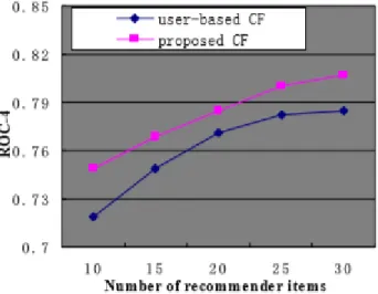
Figure 1: Comparing the proposed CF with user-based CF...14

Figure 2: Comparing factor model with popularity ranking and neighborhood model...16

Figure 3: Cumulative distribution function of the probability that a show watched in the test set falls within the top x% of recommended shows...17

Figure 4: RMSE value for each cluster value...18

Figure 5: The illustration of the proposed model [25]...20

Figure 6: Illustration of the proposed model [26]...21

Figure 7: Example of Decision Tree...23

Figure 8: Illustration of Random Forest...24

Figure 9: Illustration of SVR...25

Figure 10: Illustration of Clustering...26

Figure 11: Illustration of a single-neuron layer...27

Figure 12: Illustration of forward and backpropagation in ANNs...28

Figure 13: An example of a heterogeneous network...29

Figure 14: Number of movies each year...35

Figure 15: Popular Genre in each year...36

Figure 16: Best years for each genre...37

Figure 17: Similarity percentage between different values...42

Figure 18: Illustration of Matrix Factorization...49

Figure 19: Illustration of the proposed Artificial Neural Network...50

Figure 20: Illustration of ReLU function...50

Figure 21: Matching percentage of positive prediction with k number of movies...51

Figure 22: Matching percentage w.r.t. Genre and number of movies...52

Figure 23: Results of Matrix Factorization...61

Figure 24: Results of the Deep Learning Method...62

LIST OF TABLES

Table 1: Ratings data file format...31

Table 2: Tags data file format...32

Table 3: Movies data file format...32

Table 4: Links data file format...33

Table 7: Proposed method data file format...34

Table 8: Fifth approach file format...40

Table 9: Results of the fifth approach...54

Table 10: Results of the sixth approach with the Action genre...55

Table 11: Results of the sixth approach with the Drama genre...55

Table 12: Results of the sixth approach with the Thriller genre...56

Table 13: Results of Decision Tree with Average people...57

Table 14: Results of Decision Tree with Non-Average people...57

Table 15: Results of Random Forest with Average people...58

Table 16: Results of Random Forest with Non-Average people...58

Table 17: Results of SVR with Average people...59

Table 18: Results of SVR with Non-Average people...59

ABBREVIATIONS

ANNs Artificial Neural Networks

CF Collaborative Filtering

HIN Heterogeneous Information Network

IMDb Internet Movie Database

MF Matrix Factorization

KNN K-Nearest Neighbors

MAE Mean Absolute Error

MLP Multilayer Perceptron

MSE Mean Squared Error

RMSE Root Mean Square Error

SVR Support Vector Machine

SVM Support Vector Regression

CHAPTER ONE

1.

Introduction

In the current era of modern technology, information is increasing at a rapid pace. The amount of information available on the internet is not relevant according to the user’s preferences [27]. Most of the users spend their precious time to navigate towards useful information. Recommender systems are getting popular as e-commerce is growing rapidly in the current decade. Recommender systems are one of the best solutions to this problem. E-commerce platforms such as Netflix, Amazon Prime has millions of users with millions of items to offer [28]. It is a challenge for these companies to recommend preferred items to the user according to the user’s taste. The recommender system is one of the modern tools to solve this sort of problem in the current era. These are data filtering engines that try to recommend items that are best for their interest.

The recommender systems are normally categorized into the following types: content-based filtering, collaborative filtering, and knowledge-based filtering methods [29]. Items are recommended on a similarity basis either on a user profile or an item profile. These approaches find the similarity between similar users or similar items then similar items are suggested to the specific users according to their profiles. Recommender systems mostly rely on explicit feedback, meaning that users give explicit input regarding their interest in products. For example, Netflix collects the star rating given by the user for watched movies.

Motivation

In the current decade, hybrid systems are emerging as a successful approach in recommender systems. Hybrid systems have achieved better results compared to the previously applied conventional methods [30]. These methods have overcome the weaknesses of recommendation techniques by replacing them with the strength of another. The performance of these methods depends upon the integration technique of their components.

The items in the database are in large number and it is very difficult for any user to view or rate all items. Every user visits or rates limited number of items in the database, that generates the

sparse user-item matrix for a recommender system. It is very challenging to recommend the desired items to the specific user. Moreover, fetching the appropriate features for the items itself is the main challenge in this filed. Furthermore, for a new user in the database, we cannot recommend the personalized items as we do not know his priorities. This leads us to the cold start problem which is still the one of the major issues in the recommender systems. In this research, our goal is to recommend appropriate items to the users according to their interests. Objective

The main objective of this research is to recommend the personalized items to the users according to their interest. As the user-item matrix is sparse, it is very difficult to recommend items to the user. The sparsity of the matrix leads to a decrease in the efficiency of recommender systems as the user-item matrix does not contain enough ratings which should help recommendation. In this research, we combine different techniques such as Decision Trees, Support Vector Regression, Matrix Factorization, and Neural Networks to achieve better results. Thesis Organization

The thesis is organized as follows: The literature review is discussed in Chapter 2, while Chapter 3 describes the preliminaries of previously applied methods in the literature. Moreover, proposed approaches such as primitive and non-primitive (Machine Learning, Deep Learning, etc.) are discussed in Chapter 4 along with the description of data set briefly. Results of the proposed approaches are described in Chapter 5 and discussion about the results of the proposed methods and previously applied methods along with the future work are described in Chapter 6.

CHAPTER TWO

2.

Literature Review

In the current decade, recommender systems are highly anticipated as independent research. As the amount of data and information is increasing by the passage of time, it is hard to mine the appropriate data for the users and to recommend items according to the taste of every individual. A recommender system provides a solution by recommending appropriate items to the user by applying different techniques which we will discuss later. Furthermore, enterprises predict the

items for a recommendation of every user by their purchasing habits, watch history to make a better experience for the users [1].

In the literature, multiple techniques have been studied and applied for recommendation purposes. The techniques such as collaborative filtering and content-based filtering are most effective in recommender systems. We will discuss these techniques in detail below.

2.1. The Content-based Approach

This approach depends on the content viewed or rated by the user. For better recommendations, a user profile is generated which holds the information about the user activity and the preferences. The user profile is dependent on user preferences and their activity through the items. The profile is generated through keyword analysis, previously seen, and rated items. In general, it involves the latest activity of the user. Moreover, the recommender system analyzes the positive rated and negatively rated items in each user profile and recommends items according to the user preference. The recommended items are generally similar to the positively rated items or general high rated items in the database [4].

2.2. The Collaborative Approach

In this approach, multiple filtering techniques are used for recommendation purposes. The famous collaborative filtering techniques are item-based filtering, user-based filtering, neighborhood-based filtering, and model-based filtering. In this research, we have divided it into the following categories:

 User-based Approach  Item-based Approach  Model-based Approach

2.2.1. User-based Approach

In this approach, the user performs a major role in recommendations. The user behavior determines which items should be recommended to themselves. For example, if the user like item-A then more items will be recommended from the same category to the user. Moreover, in this approach items from the same set of users can be recommended to specific users. For example, if the user liked item-A, then the items from the same group of people who have liked item-A will be recommended to the user. This approach

determines the behavior of the same users according to liked items and then afterward items are recommended to a user according to the neighborhood [2]. Mostly, neighborhood models are used in this approach. Such user-oriented systems estimate the ratings of an item, based on the similarity of the item or users.

Pu wang and Hong wu ye proposed in [15] a collaborative filtering algorithm for

personalized recommendations of an item to the users. In this study, the slope one scheme technique is used to fill the sparsity of the user-item matrix. Afterward, it implements collaborative filtering for the recommendation of items to the users. The slope one algorithm utilizes information such as ratings of a specific item from other users and all items rated by the same user. Moreover, this process consists of two phases to produce recommendations.

i) Calculate the average deviation of the two items. ii) Calculate the prediction.

Given two items Ii and Ij the algorithm considers the average deviation Dij of item

I_i concerning item I_j as:

D_ij=

∑

R_ci−R_cj

count

(

)

(1)

where Rci is the rating given by user c to item i and Rcj the rating of user c to item

j . The second step involves predictions P_ci which are calculated by the following equation:

P_ci= 1

count (Rct≠0)R

∑

R_ct+D_ci (2)

where P_ci is the predicted rating of user c would rate item i , R_ct is the rating of all the user c to item t , and Dci is the average deviation of for item i from all users

After the implementation of the slope one scheme algorithm, the dense ratings were achieved which transformed the original sparse matrix into a dense matrix. Furthermore, for the measurement of user rating similarity Pearson’s Correlation was used to measure the correlation between two vectors of rating. Moreover, for the recommendation purpose weighted average of neighbor’s ratings was calculated according to the target user. The rating Put of the target user u to the target item t is as following:

P_ut=A_u+

∑

(

)

∑

where A_u is the average rating of the target user towards items, R_it is the rating of the neighbor of user i to the target item t , Ai is the average rating of the neighbor for user

i to the items, ¿(u , i) is the similarity of the target user u and the neighbor user i , and c is the number of the neighbors.

The MovieLens dataset was used for this research. This dataset contains ratings of movies that are rated by different users. In this research, decision-support accuracy measures are taken as it helps users to select high-quality items.

2.2.2. Item-based Approach

It is obvious that the preferences of a user remain similar or slightly changes over time so a similar approach as user-based is applied here. Items with similar ratings or content are recommended to the user. The same neighborhood method is applied to the items which recommends a similar item to the user’s preference [3].

Yifan Hu et. al proposed in [14] a model that does not consider any direct inputs from the

users regarding their preferences. In their work, the dataset was treated as an indication of positive and negative indications of an item with varying confidence levels about an item towards a specific user. In this work, they have introduced a set of binary variables that indicate the user preference pui to item i about any specific item.

p_ui=

{

(4)

In other words, if the user u has consumed the item i then the user likes the item and if

the user doesn’t consume the item then the user doesn’t prefer this item. Moreover, in this study confidence levels varies according to the behavior of the user. In the beginning, if the user liked the very first item then the confidence level will be much lower compared to a user who has liked the series of similar items. For example, a user may watch a TV show because he/she is staying on the same channel as the previously watched show. This model has a different confidence level for different users and items. But confidence level grows as the model has a stronger indication that the user likes the specific type of items. To measure the confidence level new variable was introduced. The value of confidence level increases with more user preferences about items.

The main purpose of this research was to find the vectors for each user and item. These factors are known as user-factors and item factors. This approach is similar to the Matrix Factorization technique which is also popular for explicit feedback data. In this work, two important distinctions are generated.

i) Account for a varying confidence level. ii) Optimization for all user and item pairs

Factors are computed by minimizing the following cost function: pui−xu T

‖

‖

∑

‖

_‖

∑

∑

where c_ui is the set of variables which measures the confidence level in observing the

p_ui. The right part of the equation

‖

∑

‖

∑

is designed for regularization

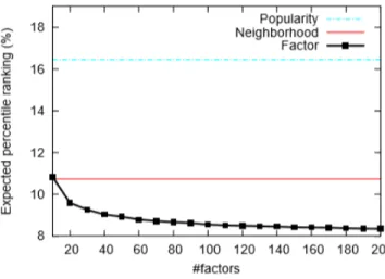
purposes to avoid overfitting the data, x_u is the user factor vectors and y_i is the item factor vectors. The value of λ is data-dependent. The implementation of the model was based on a different number of factors ranging from 10-200. The dataset was taken from digital television service. The collected data was about 300,000 set-top boxes. Evaluation of the proposed approach was done by arranging an ordered list of TV shows, sorted from one predicted to be most preferred one to the least preferred one. For the prediction of user behaviors about TV shows _rank´ _{was used:}

´ rank =

∑

∑

where r_ui are the rating of the user u to the program i and ran k_ui denotes the percentile-ranking of program i within the ordered list of all programs prepared for user u . Lower values of rank are more desirable, as they indicate rankings of watched shows closer to the top of the recommendation lists. The results are illustrated below for the proposed approach.

Figure 2: Comparing factor model with popularity ranking and neighborhood model.

Figure 3: Cumulative distribution function of the probability that a show watched in the test set falls within the top x% of recommended shows.

2.2.3. Model-based Approach

This approach uses some machine learning and deep learning algorithms to learn new ratings by analyzing the previously given ratings. These methods are very fast in computation and they can predict more accurately. Once the model is trained it can make predictions very quickly on the new data entries in the database. Examples of these techniques are included in [6] and some of the techniques are listed below.

 Random Forest  SVD

 Clustering

 Artificial Neural Networks  Link Analysis

 Hybrid Approaches

 Link Prediction Approaches

Clustering and Random Forest

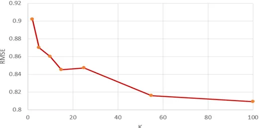
Ajesh et.al proposed a system that uses clustering and random forest algorithms for

recommendation purposes [16]. The recommendation system was designed on user ratings and the recommender system was evaluated by computing accuracy and Mean Square Error. Moreover, the users were clustered based on ratings given by users for each movie. The results of the research are illustrated in the figure below. The X-axis represents the number of clusters and Y-axis represents RMSE.

Figure 4: RMSE value for each cluster value.

Artificial Neural Networks

M. T. Ahamed proposed a collaborative filtering method which implies matrix factorization and

deep neural networks under its framework [25]. This paper proposed a recommender system where a deep neural network is replacing the inner dot product of matrix factorization that can learn non-linearities of the system. Furthermore, to incorporate the non-linearities of the system matrix factorization is combined with deep neural networks. A single user can rate multiple

items in the personalized recommender system. For this reason, unique users can be formulated against unique items and can be transformed into multidimensional space. So, user and item embeddings are used to represent the latent features of users and movies which determines the strength of the relationship for each user.

Matrix Factorization layer

In matrix factorization, the embedding for the user u and item i are denoted as p_u and

q_i respectively. Then, the dot product of pu and qi is denoted by yui and calculated as following:

^y=f

₍

₎

∑

P_ukq_ik (7)

where p_u and q_i denotes the user and item embeddings respectively. Moreover, K denotes the number of latent features for the proposed embeddings.

Multilayer perceptron layer

Moreover, a multilayer perceptron with a hidden layer is used to comprehend the interaction of latent features between users and items. The layered model under the multilayer perceptron produces an output ^y . The hidden layers are activated by ReLu function denoted by h :

^y=R

₍

(

)

)

where ∅(zL−1) is

∅

(

)

(

T

+b_L

)

where Wx, bx∧ax are the weight matrix, bias vector, and activation function respectively.

Combine MF and MLP layer

Moreover, two models Matrix Factorization and Multilayer perceptron are combined in the final hidden layer to provide more accurate results. The output of the layer is denoted by ^y :

^y=R

(

(

[

qi

]

)

)

(10)

where the activation function is denoted by R in the output layer if ReLU is used as an activation function. Furthermore, the following figure illustrates the general overflow of the model.

Figure 5: The illustration of the proposed model [25].

Xiangnan proposed a neural network approach for collaborative filtering [26]. In the proposed

approach, they replaced the inner product of Matrix Factorization with a neural network architecture that can learn an arbitrary function from the data. Multiple layers were introduced in this research. The first layer maps the embeddings of users and items to learn more features about both entities to find a powerful relationship. Moreover, neural collaborative filtering layers are used to find the most promising relationships between the entities and prediction. The workflow of this method is illustrated in the figure below.

Figure 6: Illustration of the proposed model [26].

The Hybrid Approaches

Wide and diverse techniques have been used for the recommendation systems such as collaborative filtering, content-based filtering, etc. These techniques have been blended and used for better prediction and recommendation purposes. These hybrid techniques can be designed by a mixture of two or more techniques. These hybrid approaches can be used in different ways [5].

 Individual implementation of collaborative and content-based approaches and aggregating their outcome.

 Integration of some characters from one approach with another approach.

 Weighted Approach

In this approach, the weight of the recommended item is calculated by applying all available approaches and aggerating the score. Mostly, additive aggregation is used to normalize the weight.

 Mixed Approach

Different recommendation approaches recommend a different item for a user. This hybrid approach merges all those recommendations and recommends it to the user. This technique is very useful for the cold-start problem.

Link Prediction Techniques

Nowadays, the complexity of networks is increasing and it is hard to mine appropriate information from the network. For example, take an example of recommendation systems for Twitter or Facebook, the basic aim for these applications is to recommend preferred tweets and content for every user. Many online e-commerce applications and companies need to mine information according to the user’s preferences. It is very important to mine the appropriate information for these applications [8]. The main challenge is to represent a network into a low dimension. There are different techniques to overcome this problem. The main and basic challenges are the following.

 High non-linearity  Structural preserving  Sparsity

 Cold start

Daixin Wang et al. proposed the implementation of structural Deep Network Embedding (SDNE)

to capture the high non-linear network structure [9]. This research proposed the semi-supervised deep learning model consists of multiple layers of linear functions to capture the high non-linearity of the network. Moreover, first and second-order proximity was used to preserve the network structure.

Carl Yang et al. proposed similarity modeling on heterogeneous networks via automatic path

discovery to overcome meta-paths limited path problems [11]. In this work, the purpose was to properly model node similarity in terms of content-rich heterogeneous networks. For pairs of nodes, automatic path discovery was proposed for both structural and content information. Chuan Shi et al. proposed another approach for heterogenous network embedding for HIN based recommendations called HERec [12]. To achieve meaningful node sequences for network a meta-path based random walk strategy is implemented. The node embeddings are transformed by a set of fusion functions and then integrated with matrix factorization (MF).

CHAPTER THREE

3.

Preliminaries

In this chapter, we will introduce the background of user-items interaction in multiple studies using techniques such as decision trees, support vector machines, collaborative filtering, matrix factorization, and other link analysis techniques.

3.1 Decision Trees

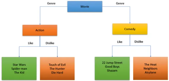
The decision tree is based on the methodology of tree graphs which are constructed on training examples. There are known class labels for which analysis is done on training data, then it is applied on the unseen examples to classify the given item.

The decision tree forms are predictive models based on the input attributes and they predict a value. Each node in the tree corresponds to an attribute and the edge from parent to child node corresponds to the value of that attribute. The construction of the tree starts with the root node and the input data. An attribute is assigned to each node and edge as the tree grows according to the given input. The given input data is then split by the appropriate values so that each child node should get the appropriate value specified by the corresponding edge. This process is repeated recursively until there is no feasible splitting required according to the given input. The following figure illustrates the simple example of a decision tree.

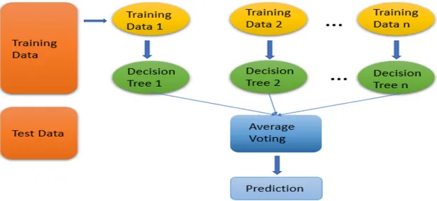
3.2 Random Forests

It’s a supervised learning method for classification and regression. It operates by constructing the multiple decision trees at training time and gives them out in the mode of classes (Classification) or mean prediction in case of (Regression) of the individual trees. In general, the more trees in the forest the better the robustness. It calculates the positive and negative predictions for a given item to be predicted. The decision depends upon the more values achieved by the algorithms by some set of rules or taking the average of results achieved. The following figures illustrate the behavior of a random forest algorithm.

Figure 8: Illustration of Random Forest.

3.3 Support Vector Regression (SVR)

It is a machine learning algorithm used for regression problems. SVR is a little different from other regression techniques. In other regression techniques, the main goal is to minimize the sum of the squared error while in SVR, the goal is to fit the error in a certain threshold. The following are the fundamental parameters for the SVR.

 Kernel

 Hyper Plane

It is the separation line between the data classes. The data points are aligned according to this line.

 Boundary Lines

These are two different lines distant from hyperplane which creates a margin of error between the data points in the model. The support vectors can be within the boundary lines or outside these lines.

 Support Vectors

These are the data points that are distributed across the hyperplane and boundary lines.

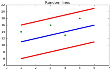
The following figure illustrates the example of SVR with boundary lines and data points scattered across hyperplane.

Figure 9: Illustration of SVR.

The red lines are the boundary lines, green dots are the data points and the blue line is the hyperplane. The main objective is to find the best fit line which contains the maximum number of data points.

Let’s say ε is the distance of boundary lines from the hyperplane by assuming that hyperplane is a straight line going through Y −axis . Let’s say the equation of hyperplane is the following:

wx+b=0

Therefore, according to the above equation, we can say that the two-equation of boundary lines are the following:

wx+b=+ε

wx+b=−ε

Thus, for any linear hyperplane, the equation which satisfies SVR is: - ε ≤ y−Wx−b ≤+ε

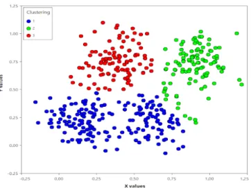
3.4 Clustering

Clustering techniques are used in multiple domains such as image processing, pattern recognition, and statistical analysis, etc. Moreover, clustering algorithms try to partition the data into sub-clusters to achieve meaningful groups with the highest similarity. Once the clusters are formed then the new user can be predicted according to the relevant cluster which contains similar users [7]. The illustration of clusters is given in the following figure.

3.5 Artificial Neural Networks

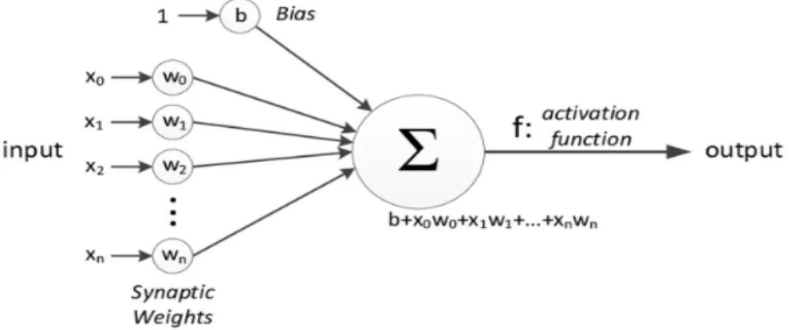
Artificial neural networks are used extensively in the field of computer vision, classification, image processing, etc. ANNs are inspired by the human mind which contains neurons. These neurons are responsible for receiving the input from outside, processing it, and giving output about a particular action. In the previous decade, researchers developed these artificial neural networks to process the data for classification and regression problems. ANNs contain layers of neurons that are connected in a symmetry. The connection between neurons has some weights to minimize the error. The ANN is robust and extensively used for the estimation of nonlinear functions and capturing complex relationships between the entities [36]. The following figure illustrates the single layer of a neural network.

Figure 11: Illustration of a single-neuron layer.

In the figure above, the inputs x0, x₁, x₂, ... , x_n are given to the neural networks. The input layer can be composed of multiple neurons depending upon the input size. The weights

w₀, w₁, w₂, … , w_n shows the strength of the particular node and b is the bias which allows the control of the activation function. The purpose of the activation function is to decide whether the neuron should be activated or not after calculating the weighing sum and adding the bias value to it. In ANNs multiple activation functions are used such as sigmoid, hyperbolic, and ReLU (Rectified Linear Units).

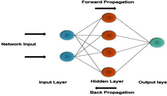
The training process of ANNs includes forward propagation and backward propagation to minimize the cost function. Every neural network layer gives output to the next layer and the

cost function is calculated. The main goal of the neural network is to minimize the cost function. The cost function is the difference between the actual value and the predicted value by the network. The resulting data is fed again and again to the neural network to minimize the cost function and this process is called backpropagation. The figure below illustrates the concept of the forward propagation and backpropagation.

Figure 12: Illustration of forward and backpropagation in ANNs.

3.6 Collaborative Filtering

For M items and K users, the profile of the users is represented in a K x M user-item matrix X . Each entry in the matrix X such as Xk , m=r indicates that user k rated item m by r , where r∈{1 , …,|r|} if the item has been rated, and Xk , m=∅ means that the rating for the movie is unknown for a specific user. The user-item matrix can be decomposed into vectors of rows: X =

_[

_]

_[

where T denotes the transpose of the given matrix. Given each row factor k , t¿

u¿

corresponds

3.7 Matrix Factorization

Recently, in the user-item factorization models are based on Matrix Factorization. The rating matrix R is the approximation of the dot product of two matrices P∧Q , where

P∈ Rn x k _{is the user latent matrix and Q∈ R}m xk _{is the item latent matrix, where k is the} total number of latent factors and k≪n,m . The prediction score of user u and item i is predicted as follows:

^

rui=puqi

T ₍₁₁₎

where p_u is the latent vector associated with the user u and q_i is the latent vector associated with the item i .

3.8 Heterogeneous information network and embeddings

A heterogeneous information network is a form of a graph, which contains sets of nodes and edges. The set of nodes and edges in such networks consist of multiple types. The following graph illustrates the heterogenous information network.

Figure 13: An example of a heterogeneous network.

The HIN use embeddings to project the nodes and edges into a low dimensional vector space. The purpose of HIN embedding is to learn a mapping function for each node in a low-dimensional space by preserving the properties of original network.

CHAPTER FOUR

4.

The proposed approach

This chapter describes the proposed approaches which are conducted for this research. Firstly, the description of the dataset is discussed in detail. It includes the file structures of different files present in the dataset. Further, different analyses have been described to better understand the data. Furthermore, primitive approaches are described in detail. Later in the chapter, different machine learning and deep learning techniques are discussed.

4.1. Dataset Description

The dataset used for this research is titled as “MovieLens” [17]. It has been collected over multiple times of duration and contains 25 million entries of ratings of movies rated by users. It includes over 62,000 movies and 162,000 users. Users have been selected randomly and every user has rated at least 20 movies. Each user and movie are represented by userId and movieId. It includes the following files listed below.

 ratings.csv  movies.csv  tags.csv  links.csv User Ids

User ids are randomly selected in the dataset and ids are anonymous. User ids are same and consistent across all the files.

Movie Ids

A unique Movie id is assigned for each movie and only those movies are attached in the dataset which is rated by at least one user. Moreover, Movie ids are consistent across all the files.

4.1.1. Data files structure

In this section, a detailed description of different data files is given. Multiple files contain information for the users and movies.

Ratings Data File Structure (ratings.csv)

The ratings given by all the users are in the ratings.csv file. Each entry in this file represents the rating of the specific movie given by a specific user. The format of this file is given below with an example:

userId movieId Rating timestamp

1 296 5 1.15E+09

1 306 3.5 1.15E+09

1 307 5 1.15E+09

Table 1: Ratings data file format.

The data in this file is ordered by userId. The scale of ratings is from (0.5 stars – 5 stars). The minimum rating for any movie is at least 0.5. The timestamp column represents the time of given ratings in seconds since the midnight Coordinated Universal Time (UTC).

Tags Data File Structure (tags.csv)

This file contains the tags created by the users. Tags are the metadata of the movies generated by users. All the tags given by the user comprises of a single word or

single phrase. Each user knows the actual meaning of his tags. The file has the following format.

userId movieId Tag Timestamp

3 260 Classic 1.44E+09

3 260 Sci-fi 1.44E+09

4 1732 Dark comedy 1.57E+09

Table 2: Tags data file format.

The data in this file are ordered by userId. The timestamp represents the seconds since the midnight Coordinated Universal Time (UTC).

Movies Data File Structure (movies.csv)

The information about all the movies is given in this file. Movies titles are imported from [18] and include release year of the movies. The file has the following format.

movieId Title genres

1625 The Game (1997) Drama | Mystery | Thriller

1645 The Devil’s Advocate (1997) Drama | Mystery | Thriller

1653 Gattaca (1997) Drama | Sci-Fi | Thriller

Table 3: Movies data file format.

There are total of 17 genres in this file. Genres are selected from the following list.  Action  Adventure  Animation  Children's  Comedy  Crime

 Documentary  Drama  Fantasy  Film-Noir  Horror  Musical  Mystery  Romance  Sci-Fi  Thriller  War  Western

 (no genres listed)

Links Data File Structure (links.csv)

This file includes different ids that can be used to link these movies to other sources and has the following format.

movieId IMDb Id tmdb Id

1 114709 862

2 113497 8844

3 113228 15602

Table 4: Links data file format.

 movieId is an identifier used by movielens organization [17].  ImdbId is an identifier used by IMDb [19].

4.1.2. Data Set for Proposed Research

For convenience, we have merged all the necessary information into a single file to conduct this research. The data is consistent through all the rows and columns. The following columns are included in our dataset for analysis.

 UserId: The unique id of users who rated the movies.  MovieId: The unique movie ids.

 Title: The title of the movie.

 Year: The release year of a specific movie.

 Genre: The category of the movie (i.e.) Action, Comedy, etc.  Rating: The rating out of 5 which users rated the specific movie.  Timestamp: The date at which the user rated the specific movie.  ImdbId: The id for the same movies generated by IMDb sources.

 IMDb rating: The rating is the average ratings of a specific movie and the scale of the rating is (0 – 10 stars).

The combined data file illustration is given below in the table.

UserI d

movieId rating title year genres ImdbI

d Imdb rating 1 3 4 Grumpier Old Men 1995 Comedy | Romance 114709 6.5

1 6 4 Heat 1995 Action | Crime |

Thriller

113277 8.3

1 47 5 Seven 1995 Mystery | Thriller 114369 8.7

1 50 5 The Usual

Suspects

1995 Crime | Mystery | Thriller

114814 8.7

Data for the Processing (Subset of Data)

The total dataset consists of 25 million rating entries. For our initial analysis, a small dataset of Movielens 100K entries is used. This dataset was obtained from [17] and it is consistent. On the other hand, for machine learning approaches such as Support Vector Regression, Decision Trees, and Random Forest, another subset of 25M entries dataset is used in which this subset consists of the 1st _{one million and the 2}nd _{one million} entries approximately [37]. We have tested the above-mentioned approaches on both of these sub-datasets. Moreover, the results mentioned in the respective approaches belong to the 2nd _{one million entries of the original dataset of 25M entries. The subset of the data} is sequential and consistent throughout the implementation. The results for both of these subsets of the data were almost the same.

A similar dataset is used for approaches such as Collaborative Filtering, Matrix Factorization, and Artificial Neural Networks. The results obtained in this research from these approaches were also obtained by the 2nd _{one million entries of the original dataset.}

4.1.3. Analysis of Dataset

In this part of the chapter, multiple analyses have been conducted to better understand the data for learning purposes.

The dataset contains movies from the year 1902-2018. There are a different number of movies released in different years. In the graph below, we can determine easily which

year was more productive in releasing the total number of movies.

Figure 14: Number of movies each year.

Popular Genre in every year

The popularity of the genre is considered based on the number of movies released in a specific year for a specific genre. In the dataset, some movies belong to more than one genre so, we have considered those movies in every mentioned genre. In the graph below, every popular genre is mentioned in every year.

Figure 15: Popular Genre in each year.

The above figure illustrates that people always have loved drama movies in previous decades. If we look at recent years it is obvious that producers are making comedy movies. These trends show that drama and comedy movies were always popular among users. These trends help to recommend items to the users in the cold-start problem.

Best years for each Genre

The popularity of the genre is considered based on ratings given by each user to each movie. Afterward, the mean of all given ratings for each genre movie was calculated. The highest mean value of ratings indicates that the specific genre was popular in that specific year. As in the dataset, onemovie belongs to multiple genres, so we have considered that movie in every genre. In the graph below, every popular genre is illustrated for every year.

Figure 16: Best years for each genre

4.2. Primitive Approaches

In this section, different primitive approaches are described to achieve the similarity index between the users, based on common movies. The goal is to achieve maximum positive prediction for a user movie rating. During the time of research, multiple approaches were

considered to achieve better results. Further below, we will discuss all the primitive approaches that were applied to this dataset for a better understanding of the data.

4.2.1First Approach

In this scenario, we are predicting the similarity between different users with respect to different random movies. Our goal is to achieve the maximum similarity between the users based on movie ratings. For this purpose, we assume the following approach.

1. Pick two random movies M1∧M2 .

2. Determine the corresponding common users for these two movies. 3. If the number of such users is not at least 3, then go back to step (1). 4. Otherwise, take 3 common users.

5. Use their ratings to determine similar behaviors.

Let’s say for M₁ the users are A , B ,∧C with corresponding ratings r_A, r_B∧r_C , respectively. Similarly, for M2 the same users A , B ,∧C have the corresponding ratings r_{A 1}, r_{B 1}∧1 , respectively. For each movie and set of users, assign 1

¿r_{A 1}−r_{B 1}∨≤∨r_{B 1}−r_{C 1}∨¿

i f

_|

_|

_|

_|

4.2.2 Second Approach

In this scenario, we predict the similarities between two users with respect to different random movies. Our goal is to achieve the maximum similarity between the users on the ratings of movies. For this purpose, we assume the following approach.

1. Take two random users A∧B . 2. Find all common movies for them.

3. Take the difference of ratings between these two users for M₁ , call it as DAB 1

. 4. Take the average difference of ratings between these two users for M₁ and M₂ . 5. Take the average of differences between the rating for n−1 movies.

6. Compare the last movie rating difference with the average difference between two users for all movies.

Let’s say for M1 the users are A∧B with corresponding ratings rA∧rB , respectively. Similarly, for M₂ , same users A∧B have the corresponding ratings

r_{A 1}∧r_{B 1}, respectively. The difference between r_A−r_B is called D1AB and the last common movie is DAB

n

, respectively and the average difference between two users across all movies is Avg (Dn−1AB ) . If the difference of last common movie DnAB between A∧B is somewhere between 0 ≤ DABn ≤ Avg (Dn−1AB ). Then, take it as a positive case, otherwise negative.

4.2.3 Third Approach

In this scenario, we predict the similarities between two users with respect to multiple random movies (k =1,2,3 , … ,10) . Our goal is to achieve maximum similarity between the users on the ratings of movies as we increase the number of common movies between the two users (k =1,2 ,…, 10) . For this purpose, we assume the following approach. 1. Take two users A and B with common movies.

2. Look at their difference of ratings for M1 , call it DAB1 . 3. Look at their difference of ratings for M2 , call it D2AB . 4. Look at their difference of ratings for M₃ , call it D3AB .

5. Then if their difference of ratings for M₄ is somewhere between 0 ≤ DAB

4

≤ Avg

(

)

Let’s say for M1 the users are A∧B with corresponding ratings rA, rB respectively. Similarly, for M₂ the same users A∧B have the corresponding ratings rA 1, rB 1 respectively. The difference between rA−rB is called D1AB and the last common movie is DkAB respectively and the average difference between two users across all movies is Avg (DAB

k−1

) . If the difference of last common movie DAB k between A∧B is somewhere between 0≤DkAB≤Avg(Dk−1AB ). Then take it as a

positive case, otherwise negative. The concept here is by increasing the number of common movies between them we can achieve more positive predictions.

4.2.4 Fourth Approach

In this scenario, we predict the similarities between two random users with respect to different common movies within range of k, where (k =1,2,3 , … ,10) . The concept here is to increase the number of movies in every iteration. Furthermore, a specific genre is selected to maximize the similarities between two users based on the given information in the above-mentioned combined dataset. As the data is heterogeneous, the goal is to achieve better results by including useful and necessary information. The main purpose is to achieve maximum similarity between the users on the ratings of movies. For this purpose, we assume the following approach.

1. Take two users A, B with different number of common movies. In this particular scenario common movies belong to the same genre.

2. Look at their difference of ratings for M₁ , call it DAB 1

. 3. Look at their difference of ratings for M2 , call it D2AB . 4. Look at their difference of ratings for M₃ , call it DAB

3 .

5. Then if their difference of ratings for M₄ is somewhere between 0 ≤ DAB4 ≤ Avg

(

)

Let’s say for M1 the users are A∧B with corresponding ratings rA, rB respectively. Similarly, for M₂ the same users A∧B have the corresponding ratings rA 1, rB 1 respectively. The difference between rA−rB is called D1AB and the last common movie is DAB

k

respectively and the average difference between two users across all movies is Avg (Dk−1AB ) . If the difference of last common movie DkAB between A∧B is somewhere between 0 ≤ DABk ≤ Avg (Dk−1AB ). Then, take it as a positive case, otherwise negative. The concept here is by increasing the number of common movies between them we can achieve more positive predictions.

4.2.5 Fifth Approach (Inclusion of IMDb ratings)

In this particular approach, the IMDb ratings are included in the original dataset. The key concept is to compare user ratings with IMDb ratings. The IMDb ratings are rated from the scale of 1 star to 10 stars [19]. These ratings are given by the users on the IMDb platform. These ratings are the average ratings for a specific movie. The original dataset rating scale is (1-5 star) and the IMDb rating scale is (1-10 star). It is necessary to normalize the original ratings with IMDb ratings. After including IMDb ratings and normalizing the original data is illustrated in the table below.

userId movieId rating Imdb rating

title genres Imdb

Id

2 318 6 9.3 Shawshank

redemption

Crime | Drama 111161

2 106782 10 8.4 The wolf of wall

street

Comedy | Crime | Drama

993846

2 89774 10 8.3 Warrior Drama 1345836

Table 6: Fifth approach file format.

Average Users

The concept of average users originates with a comparison of user original rating and IMDb rating. To decide whether the user is average or non-average, the dataset is tested on multiple values for optimization.

Non-Average Users

The non-average users’ ratings are different from overall IMDb ratings of the movies given by the users. These users contain different behavior while rating the movies.

Criteria

The criteria is selected in such a way that it includes at least 10% of the total users in average users. Average users are selected according to the following criteria.

 The difference between user rating and IMDb rating should be ≤ 1.5. For example, the user A has rated k many movies. We calculate the difference of movies

M₁, M₂, … , M_k rated by user A with respect to IMDb ratings such that

r_{A → M1}−r_{imdb→ M}

1≤1.5 .

 The number of movies satisfying the above criteria should be at least 80%.

 All the users who are not satisfying the above two criteria belong to non-average people. Below, the figures illustrate the number of people changing with the number similarity percentage. As we increase the similarity percentage from ( 10 , … ,100¿ the number of users is decreasing as expected for the specific difference mentioned above.

Figure 17: Similarity percentage between different values.

1. Take two random users A and B from the set of average and non-average people separately in different intervals i. e .

¿ I90−100, I80−90, … , I0−10¿ . 2. Take k common movies (i. e . M1, M2, M3, M4, … , Mk) . 3. Look at their difference of ratings for M1 , call it as D1AB . 4. Look at their difference of ratings for M₂ , call it as DAB

2 . 5. Look at their difference of ratings for Mk−1, call it as Dk−1AB .

6. Then if their difference of ratings for Mk is somewhere between 0 ≤ DABk ≤ Avg

(

)

Let’s say for M₁ the users are A∧B with corresponding ratings r_A, r_B respectively. Similarly, for M2 the same users A∧B have the corresponding ratings rAA, rBB respectively. The difference between r_A−r_B is called D1AB and the last common movie is

DkAB respectively and the average difference between two users across all movies is

Avg (DAB k−1

) . If the difference of last common movie Dk_AB between A∧B is somewhere between 0 ≤ DABk ≤ Avg (Dk−1AB ). Then, take it as a positive case, otherwise negative. Repeat this process for each interval.

4.2.6 Sixth Approach

This approach is similar to the above (fifth approach) but the genre is included. The ideology remains the same that by including more information better results can be achieved. The results of some main genres are included below.

1. Take two random users A and B from the set of average and non-average people at different intervals i. e .

¿ I90−100, I80−90, … , I0−10¿ with one genre (i.e. Action, Comedy, Drama, etc.).

2. Take k common movies (i. e . M1, M2, M3, M4, … , Mk) . 3. Look at their difference of ratings for M₁ , call it as D1AB . 4. Look at their difference of ratings for M2 call it as DAB

2 . 5. Look at their difference of ratings for M_k−1 call it as DAB

k−1 .

6. Then if their difference of ratings for M_k is somewhere between 0 ≤ DABk ≤ Avg

(

)

Let’s say for M1 the users are A∧B with corresponding ratings rA, rB respectively. Similarly, for M₂ the same users A∧B have the corresponding ratings rAA, rBB respectively. The difference between rA−rB is called D1AB and the last common movie is DAB

k

respectively and the average difference between two users across all movies is Avg (Dk−1AB ) . If the difference of last common movie DkAB between A∧B is somewhere between 0 ≤ DABk ≤ Avg (Dk−1AB ). Then, take it as a positive case, otherwise negative. Repeat this process for each interval.

The implementation of all the above primitive approaches shows that better results can be achieved by filtering the data. Moreover, the results indicate that it is very hard to achieve accuracy by more than 60% in any above-mentioned approaches.

In the next section, multiple machine learning methods are implemented to achieve better results. We will compare the results of our approach to other approaches.

4.3. Machine Learning Methods

In this section, we will discuss different machine learning methods implemented in the dataset. As mentioned in the above section the dataset is divided into two categories: Average users and Non-average users. We implement different machine learning algorithms on both average and non-average users.

We apply three machine learning algorithms for testing purposes.  Decision Trees

 Random Forest

 Support Vector Regression (SVR)

We then calculate Mean Square Error as well as Mean Absolute Error as an evaluation matrix. Decision trees have been used in recommender systems as a model-based approach. Decision trees work on the parent-child node methodology for decision making. We implement this methodology for both average and non-average users for each difference i. e .2.0 – 1.5

¿ )

between user rating and IMDb ratings. From the dataset, 70% of the dataset is used for training the model and 30% of the data is applied for testing purposes. We compute both MSE and MAE for model evaluation.

Random forest is a supervised machine learning algorithm that is used for classification and regression problems. In this research, the implementation of random forest is applied both on average and non-average users as mentioned in the earlier section. From the dataset, 70% of the dataset is used for training the model and 30% of the data is applied for testing purposes. A total of 300 estimators are used for the model evaluation. Moreover, Mean Absolute Error and Mean Squared Error is calculated for the accuracy of the model.

SVR is a machine learning algorithm used for regression problems. SVR is a little different from other regression techniques. In other regression techniques, the main goal is to minimize the sum of the squared error while in SVR, the goal is to fit the error in a certain threshold. A total of 70% dataset is used for training purposes and 30% of the data is used for testing purposes. To evaluate the model, Mean Absolute Error and Mean Squared Error metrics are used.

4.4. Collaborative Filtering

In this section, we discuss the implementation of collaborative filtering methods applied to the dataset. Collaborative filtering has been very popular in the e-commerce market and the results obtained are competitive with advanced methods such as neural networks, etc. In this methodology, user-based collaborative filtering is considered. It is a technique that filters the items for users with respect to the behaviors of the user. It works by searching the large set of users from the database and find a smaller set of users who have similar behaviors towards items. This methodology personalizes the score for each user with respect to each given item. Firstly, we have to calculate the average rating of a specific item given by all users. The average rating will help to calculate the deviation of the user rating from the average rating of a specific item. The average rating s(j) of an item is calculated as follows:

s ( j)=

_∑

i∈Ωj

r_ij (12)

where Ω_j set of all users who rated movie j and r_ij is the rating that the user i rated the item j . User can rate multiple items so we have to personalize the score of each item for a specific user s(i, j) as follows:

¿Ω_j∨¿ s (i, j)=

∑

where s (i , j) is dependent on both user i and item j , ri'_j is the rating user i

rated to item j , i=1 , … , N , and j=1, … , M . Our rating matrix R_{N x M} is a user-item rating matrix of size N x M . Afterward, we have to calculate the predicted rating for item

j which is not rated by user i . As we are dealing with a real number then our objective is

to calculate Mean Squared Error. ¿Ω∨¿+

∑

(

₎

where rij is the original rating and ^r_ij is the predicted rating of the specific movie.

The above approach has a problem with the average rating as it treats every user rating equally. For example, user A rating s(i , j) equally depends on user B and user C even though user A doesn’t agree with both of the users B∧C ( i. e . user A didn’t like the specific movie j and user B and C liked). Moreover, user A interpretation can be different from user B in rating the movies. For example, user A rated 5 for liked movies and 3 for unliked movies. Whereas, user B rated 4 for liked movies and 1 or 2 for unliked movies.

The above problem can be minimized by introducing weights. For example, if user A does not agree with other users for item j then the weight will be small otherwise large. It means that we should not care about the absolute rating but we should consider how much user A

deviates from its average rating. For example, if the user A average rating is 2.5 and his rating for item j is 4, it means he likes that item. We can calculate the deviation dev (i, j) for a specific item as follows:

dev (i, j)=r (i, j)− ^r_i (15)

where r (i, j) is the original rating given by the user and r^_{i is the average rating of the user.}

Further, we can calculate the average deviation of all users for specific movie j as

^

dev(i, j) . This will give us the prediction deviation of the specific movie j :

¿Ωj∨¿+

∑

(

₎

where ´ri' is the average rating of every user. Afterward, predicted rating for item j can be