Examination of Sets of Points and Non-Null Lines Under the Two-Parameter Lorentzian Motion

(1)

EXAMINATION OF SETS OF POINTS AND NON-NULL LINES UNDER

THE TWO-PARAMETER LORENTZIAN MOTION

GULSUM YELIZ SENTURK1, SALIM YUCE2 _________________________________________________

Manuscript received: 10.03.2020; Accepted paper: 02.04.2020; Published online: 30.06.2020.

Abstract. In this paper, firstly, we interested in finding the relationships among the densities of sets of collinear points, among the densities of non-collinear points and among the densities of sets of intersecting non-null lines in Lorentzian plane. Furthermore, we concerned with the density formulas of sets of points and the sets of non-null lines under the two-parameter planar Lorentzian motion.

Keywords: point density, line density, two-parameter motion, Lorentzian plane.

1. INTRODUCTION

Between the years 1935 and 1939, W. Blaschke and his colleagues presented a series of 'Integral Geometry' presentations at the Mathematical Seminars at the University of Hamburg. Thereafter, W. Blaschke published this work in book entitled "Vorlesungen über Integralgeometrie" [1]. In this book, he gave the density for sets of points/lines and the geometric meanings of the integrals of these differential forms. Undoubtedly, his studies have been accepted as the main classical references for integral geometry. Integral geometry has improved by the researchers of W. Blaschke, A. Weil, S. S. Chern, L. A. Santalo. After their contributions, numerous studies have been examined on integral geometry in Euclidean and non-Euclidean planes/spaces. L. A. Santalo published the book "Integral geometry and geometric probability" which is one of the comprehensive books on this area [2]. He, who is one of the student of W. Blaschke, referred both classical and modern Euclidean and non-Euclidean integral geometries. The products of the densities of sets of points/lines are given in [2]. Using the studies [2, 3], G. S. Birman introduced the equivalent expressions of some of the formulas of integral geometry in the Lorentzian plane [4]. The densities for a set of points and non-null lines and the products of the densities of sets of points and non-null lines are defined in the Lorentzian plane by Birman [4].

Kinematically, the two-parameter planar Lorentzian motions are introduced with different but equivalent definitions and examined with different viewpoint in the studies [5-7]. The geometry of such a two-parameter motion of points, objects/bodies and systems of objects/bodies has a number of applications in physics, bio mechanics, geometric design and trajectory of robotics. In [8], the authors give the density formulas for the sets of points and lines under the two-parameter planar Euclidean motion and obtain the connection among the densities of the sets of points and among the densities of the sets of intersecting lines under the two-parameter planar Euclidean motion.

1_{Istanbul Gelisim University, Faculty of Engineering and Architecture, Department of Computer Engineering,} 34310, Avcılar, Istanbul, Turkey. E-mail: gysenturk@gelisim.edu.tr.

2

Yildiz Technical University, Faculty of Arts and Sciences, Department of Mathematics, 34220 Esenler, Istanbul, Turkey. E-mail: sayuce@yildiz.edu.tr.

(2)

We wish to investigate the relations between the densities of sets of collinear/non-collinear points and intersecting non-null lines under the two-parameter planar Lorentzian motion. Due to these, firstly, we give the the relations between the densities of sets of collinear/non-collinear points and intersecting non-null lines in the Lorentzian plane. After that, we define the density formulas for sets of points and non-null lines under the two-parameter planar Lorentzian motion. Using all these results, we finally get the relations between the densities of sets of collinear/non-collinear points, the relations between densities of sets of intersecting non-null lines, the product of the densities of sets of points and non-null lines under the two-parameter planar Lorentzian. Under the motion, the density of points, except for the pole points, and the density of non-null lines, except for the polar axes, are not invariant. This leads to differences in our study. Since Lorentzian plane geometry has similarities and differences from the Euclidean plane geometry, this situation is much more complicated than the Euclidean case.

2. PRELIMINARIES

This section presents some basic notions on density of sets of points and non-null lines and two-parameter planar motions in the Lorentzian plane.

2.1. BASIC NOTATIONS

The Lorentzian plane is the vector space 2 provided with Lorentzian inner product , _L given by

1 2 1 2

, ,

L

X Y x x y y where X x y and ( , )₁ ₁ Y x y . Since ,( ,₂ ₂)

L is an indefinite metric, a vector X in the

Lorentzian plane can have one of three casual characters: it can be spacelike if , _L 0

X X  or V 0; timelike if X X, _L 0; null(lightlike) if X X, _L 0 [3].

Definition 1: The measure of a set A of points X x y( , ) in the Lorentzian plane is defined by the Lebesque integral of the differential form

dX dxdy, (1) over the set A , i.e., ( ) .

A

m A 



d X The differential form in the equation (1) is called the density for points X [4].

Definition 2: A timelike line (or a spacelike line) with respect to the coordinate system { ; , }O l l₁ ₂ in Lorentzian plane is denoted by L (or _t L ) and it is defined by the _s equation

cosh sinh (or sinh cosh )

(3)

with the Hesse-coordinates ( ,p ), where p is the distance from the line L (or _t L ) to the _s origin and   [4].

Definition 3: The measure of a set B of non-null lines L p( ,) in the Lorentzian plane is defined by the Lebesque integral of the differential form

,

dLdp d over the set B , i.e., ( ) .

L

m B 



dL The differential form $dL$ is called the density for non– null lines L [4].

Let X x y( , ),₁ ₁ Y x y be sets of points and ( ,₂ ₂) L p( ,) be a set of non-null lines passing through these points in the Lorentzian plane . The pairs of points X Y, can be determined by the four coordinates x y x y , as well as by the Hesse-coordinates ₁, ,₁ ₂, ₂ p, of the non-null line L and the distances  ₁, ₂ from the points X Y, to the foot H of the perpendicular from the origin O to L . The density for a pair of points dX dY

dX dY   ₁ ₂ dLd₁d₂ (2) can be calculated in two ways depending on whether the line L is timelike or spacelike, respectively. We write the absolute value of  ₁ ₂, because all densities are assumed to be positive.

Note that the equation (2) is the same expressions as the density of a pair of points in Euclidean plane [4].

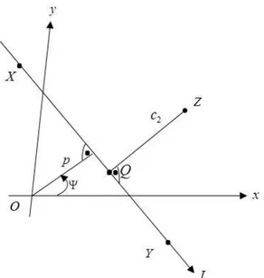
Let L p_i( ,_i _i),i1,2, be two sets of different non-null lines that intersect at the points ( , )

X x y and make angles  ₁, ₂ with the x axis in Fig. 1, respectively. The density for a pair of non-null lines L and ₁ L can be investigated in three ways depending on whether the ₂ lines are timelike or spacelike.

(4)

i. A pair of timelike lines

Let ( , ), 1, 2

i

t i i

L p  i , be two sets of timelike lines that intersect at the pointsX x y( , ). Hence, we can write

1 2 1 1 1 2 2 2 ... cosh( ) sinh( ) , ... cosh( ) sinh( ) , t t L x a y a p L x a y a p            

for the timelike lines, where a . Since, d  ₁ d ₁,d  ₂ d ₂ can be written, we get





1 2 sinh 2 1 1 2,

t t

dL dL     dX    d d (3)

for the density of a pair of timelike lines [4]. ii. A pair of spacelike lines

If ( , ), 1, 2

i

s i i

L p  i , are two sets of spacelike lines that intersect at the pointsX x y( , ), then we have the following equation for the density of a pair of spacelike lines [4]





1 2 sinh 1 2 1 2.

s s

dL dL     dX    d d (4)

iii. A pair of timelike and spacelike lines

Note that, unlike the article [4], if L p_t( ,₁ ₁) and L p_s( ₂,₂) are sets of timelike lines and spacelike lines that intersect at the points X x y( , ), we can write for the density of a pair of timelike and spacelike lines,

dL_t dL_s cosh



  ₁ ₂



dX   d ₁ d ₂. (5) 2.2. TWO-PARAMETER PLANAR LORENTZIAN MOTIONS

Definition 4: Let and  be moving and fixed Lorentzian planes; and



O l l; ,₁ ₂



and



O; ,l l₁ ₂



be their orthonormal coordinate systems, respectively. Let us take the point

( , )

X x y  and X x y  ( , )  with respect to the moving and the fixed coordinate systems. A general planar Lorentzian motion is given by the equations

1 2

cosh sinh cosh sinh ,

sinh cosh sinh cosh .

x x y u u

y x y u u

        

         (6) If , ,u u₁ ₂ are given by continuously differentiable functions of parameters t and ₁ t , ₂ then the motion is called as two-parameter Lorentzian motion / . We denote this motion

(5)

briefly by H . Here, if _II t and ₁ t are functions of the parameter ₂ t, then one-parameter planar Lorentzian motion H is obtained [5]. _I

Two-parameter planar Lorentzian motion given by the equation \ref{x'} can be written in the form

T (7) where, ASO(2,1), a u₁cosh u₂sinh, b u₁sinh u₂cosh and X and X are the position vectors of the same point X x y( , ) with respect to the moving and fixed coordinate systems, respectively, and C is the translation vector of the motion. The general planar motion is defined by the combination of a rotation and translation.

By taking derivatives the equation (7), we get X dAX A X dC

d d

where the velocities V_adX,V_f dAX dC,V_r dX are called as absolute, sliding and relative velocities of the point X [5].

Let X x y  ( , ) be the image of the point X and

... cosh sinh , ... sinh c ' o h ' s , t s L x y p L x y p              

are the images of timelike line L p_t( ,) and spacelike line L p_s( , ) under the motion H , _II respectively, where, L_t'(p ,) is defined with helps of the direction angle      and the distance p  p u₁cosh u₂sinh from the origin O Similarly, '. L_s'(p ,) is defined with helps of the direction angle      and the distance

1sinh 2cosh

p  p u  u  from the origin O [9]. '

3. ON THE DENSITY OF A SET OF POINTS IN THE LORENTZIAN PLANE

In this original section, our purpose is to give the relations between the densities of sets of points in the Lorentzian plane .

3.1 THE RELATION BETWEEN THE DENSITIES OF THE SETS OF POINTS

Theorem 5: Let X x y and ( , )₁ ₁ Y x y be sets of different points, ( ,₂ ₂) L p( ,) be a support function the points X and Y , namely, L p( ,) be a set of non-null lines that passes through these points. Let take  as a distance function from X to Y in the Lorentzian plane

. In this case, we can write

, , ,

L L

(6)

for density of a set of points Y , where dX (dx dy, ) is the relative velocity vector of the points X , u is the directrix vector and n is the normal vector of the line L p( ,).

Proof: Our aim to find the density of a set of points Y with the density of the set of points X . The theorem is another way of finding the density of the points Y . This proof will be divided into two parts depending on whether the line L is timelike or spacelike, respectively.

i. Let L p_t( ,) be a timelike line that passes through these points. In this case, the coordinates of the points Y can be written as



x y2, 2

 

 x1sinh,y1cosh



,

where u



sinh,cosh



is the directrix vector of the timelike line L p_t( ,). Thereby, we have the following equation for the density of the set of points Y ,

, _L , _L ,

dY dXd d n dX d  u dX  d (9) where dX (dx dy, ) is the relative velocity vector of the points X , n



cosh,sinh



is the normal vector of the timelike line L p_t( ,).

ii. Let L p_s( , ) be a spacelike line that passes through these points. So, we have

, , ,

L L

dY dXd d n dX d  u dX  d

for the density of the points Y , where n



sinh,cosh



is the normal vector and



cosh ,sinh



  

u is the directrix vector of the spacelike line L p_s( , ) .

Corollary 6: Let X x y and ( , )₁ ₁ Y x y be sets of different points, ( ,₂ ₂) L p( ,) be a set of non-null lines that passes through the points X Y, . Let take  as a constant distance function from X to Y . In this case, we get

, _L ,

dY dX  u dX  d

for the density of a set of points Y , where dX (dx dy, ) is the relative velocity vector of the points X , u is the directrix vector of the line L p( ,).

3.2 THE RELATION BETWEEN THE DENSITIES OF THE SETS OF COLLINEAR POINTS

dXY,

where ( ,1 ) is the barycentric coordinate of the points Q with respect to the system



O X Y , M is a set of middle points of , ,



XY and dXY a mixed point density of the points X and Y .

Proof: Using the barycentric coordinate system with respect to the system



O X Y , , ,



the following equation can be written



1



.

 

  

Q X Y

Hence, we can write the following equation for the density of the set of points Q





2







2

1 2 2 1

1 1 .

dQ dX   dY   dx dy dx dy (10) Here are another two ways of stating the equation (10):

i. Let M be a set of middle points of XY. Then, we get the following equation

1 2 1 2 _.

2 2

x x y y

dM d_  _d_  _

   

for density of the points M . Using this equality, we have

4dMdX dY dx₁dy₂dx₂dy₁. (11) Substituting the equation (11) into the equation (10), we obtain



2 1





1 2



1



4



1



,

dQ  dX   dY   dM

ii. Let dXY be a mixed point density of points X and Y which defined by the equation

dx₁dy₂dx₂ dy₁dXdY



dx₂ dx₁

 

 dy₂ dy₁



dXY. (12) Substituting the equation (12) into the equation (10), we have



1





1



,

dQdX  dY   dXY for the density of the set of points Q.

Note that the Theorem 7 is the same expressions as the density of a pair of points in Euclidean plane [8].

(8)

3.3 THE RELATION BETWEEN THE DENSITIES OF THE SETS OF NON-COLLINEAR POINTS

Figure 2. Non-collinear points in the Lorentzian plane

Theorem 8: Let X x y Y x y and ( , ), ( ,₁ ₁ ₂ ₂) Q x y be sets of collinear points and ( ,₃ ₃)

1 1

( , )

X x y , Y x y and ( ,₂ ₂) Z z z be sets of non-collinear points, ( , )₁ ₂ c be a constant distance ₂ from Q to Z and L p( ,) be a support function of the points X and Y in the Lorentzian plane . Then, we have

dZdX  



1 



dY



1



dXYc dL₂ , (13) for the density of a set of points Z , where ( ,1 ) is the barycentric coordinate of the point

Q with respect to the system



O X Y and dXY is a mixed density of points X and Y . , ,



Proof: The aim of this theorem is to find the density of the set of points Z by using the densities of sets of points X and Y , in Fig.2. The proof will be divided in two ways depending on whether the line is timelike or spacelike, respectively.

i. Let L p_t( ,) be a set of timelike lines that passes through the points X , Y . Since using the barycentric coordinate system, the vector equation













X x y and make angles  ₁, ₂ with the x axis, respectively, in the Lorentzian plane . The main idea of this section is to give the density of the set of lines L with the density of the ₁ set of lines L . This section will be divided in three cases depending on whether a pair of ₂ timelike lines, a pair of spacelike lines and a pair of timelike line and spacelike line.

i. A pair of timelike lines Let ( , ), 1, 2

i

t i i

L p  i , be two sets of timelike lines that intersect at the pointsX x y( , ). The density of the set of lines

1 t L is





1 cosh 1 sinh 1 1, t dL  dx  dy   d or

































1 2 2 2 2 2 2 2 2 2 cosh sinh

cosh cosh sinh

sinh sinh cosh ,

t dL dx dy d dx dy d dx dy d                  _       _  _       _ (14) where        ₁ ₂ ₁ ₂ . Let 2 t

L  be set of spacelike lines which is orthogonal to the set of lines

2

t

L and X x y( , ) be a intersection points of them. It can be given by the Hesse form xsinh ₂ ycosh ₂ p₃. Here is the another form of the equation (14):

1 cosh 2, 2 sinh 2, 2 ,

t L t L t

dL  _ n dX ddL _ _ u dX ddL _

where dX (dx dy, ) is the relative velocity vector of the points X , u₂ 



sinh₂,cosh₂



is the directrix vector and n₂ 



cosh₂,sinh₂



is the normal vector of the lines

2

t

L .

ii. A pair of spacelike lines Let ( , ), 1, 2

i

s i i

L p  i , be two sets of spacelike lines that intersect at the points ( , )

X x y and

2

s

L  be a set of timelike lines which is orthogonal to the set of spacelike lines to

2

s

L that intersects at the same points. Then, we have

1 cosh 2, 2 sinh 2, 2

s L s L s

(10)

for density of the lines

1

s

dL , where dX (dx dy, ) is the relative velocity vector of the points X , n₂ 



sinh₂,cosh₂



is the normal vector and u₂ 



cosh₂,sinh₂



is the directrix vector of the lines

2

s

L .

Let L p_t( ,₁ ₁) be set of timelike lines and L p_s( ₂,₂) be set of spacelike lines that intersect at the points X x y( , ) and L_s be orthogonal to set of spacelike lines L that _s intersects at the same points X . Then, we have the following equation for density of the lines

t L 2 2 cosh , sinh , , t L s L s dL  _ u dX ddL_ _ n dX ddL _

where dX (dx dy, ) is the relative velocity vector of the points X , n is the normal and 2 u 2

is the directrix vectors of the lines L . _s

5. ON THE DENSITIES OF THE SETS OF POINTS UNDER TWO-PARAMETER PLANAR LORENTZIAN MOTION

In this original section, as a beginning we give the density for a set of points X x y  ( , ) in the fixed Lorentzian plane . Following, Section 3 has been examined under the motion

II

H . Namely, we investigate the relationships between densities of the sets of collinear and non-collinear points under the motion H_II  / .

5.1 THE DENSITY FOR A SET OF POINTS

The purpose of this section is to find the density of a set of points X with the density of the points X and the components of the motion H . II

Theorem 9: Let X x y( , ) be set of points and X x y  ( , )  be an image of the set of points X under the motion H_II  / . In this case, the density of a set of points X in fixed plane  is





, _L , _L det , ,

dXdX dO_ XdX  X dO _  d dX dO (15)

where dX (dx dy, ) is the relative velocity vector of the points X , dO (du du₁, ₂) is the relative velocity vector of the points O and  is rotation angle of the motion.

(11)

dXdxdy. (16) By taking differential of the equation (6) and substituting this into the equation (16), we get



















1 12

 

2 1 1



. 2 2 dX dX x u dx d d du y u dy d d du du du dx du du dy                       (17)

If we calculate the density of points O', we can see that



1 2

 

2 1



1 2 1 1 2 2 .

dO  du u d  du u d du du u du   d u du  d (18) Using the equation (18), we get the following equation





, _L , _L det , .

dXdX dO_ XdX  X dO _  d dX dO

for the density of the points X', where det



dX,dO 



dxdu₂ dydu₁. This finishes the proof.

Corollary 10: The density of a set of pole points P in Lorentzian plane is equal to the density of a set of pole points P in Lorentzian plane . P represent the point P with respect to the fixed coordinate system under the motion H . Moreover, this density is _II zero,

0. dPdP

5.2 THE RELATION BETWEEN THE DENSITIES OF THE SETS OF POINTS

We can now give the analogue of the equation (8) in the Lorentzian plane .

Theorem 11: Let X x y and ( , )₁ ₁ Y x y be sets of different points, ( ,₂ ₂) L p( ,) be a non-null support function of the points X Y, . Let take  a distance function from X to Y in the moving plane . Under the motion H , let _II L p  ( ,) be an image of the lines L and

1' 1'

( , )

X x y , Y x( ₂',y₂') be images of the points X Y, . In this case, the density of a set of points Y is '

, _L , _L ,

dYdX d   d  n d X d  u d X  d 

where dX (dx dy₁', ₁') is the absolute velocity vector of the points X and n is the normal  and u is the directrix vectors of the lines L . 

(12)

Figure 3. Under the motion H_II, X and Y points and non-null line L.

Proof: The main idea of this theorem is to give the density of a set of points Y by using the density of a set of points in the Lorentzian plane . We first say that the distance from X to Y is equal to the distance from X to Y, in Fig.3. The proof will be given in two ways depending on whether the line is timelike or spacelike respectively.

i. Let L p_t( ,) be a set of timelike lines that passes through the points X ,Y and , )

' (

t

L p  be an image of timelike line L under the motion _t H . Similarly as in the _II equation (9), it is easy to check that

, ,

L L

dYdX d   d  n d X d  u d X  d  is obtained for the density of the points Y in the Lorentzian plane .

ii. This case follows by the same method as before.

Corollary 12: Let X x y and ( , )₁ ₁ Y x y be sets of different points, ( ,₂ ₂) L p( ,) be a set of non-null lines that passes through the points X Y, . Let take  as a constant distance function from X to Y in the moving plane . Under the motion H , let _II L p  ( ,) be an image of the line L and X x y( ₁', ₁'), Y x( ₂',y₂') be images of the points X Y, . The density of a set of points Y

, _L

dYdX u d X  d ,

where dX (dx dy₁', ₁') is the absolute velocity vector of the points X and u is the directrix  vector of the lines L .

5.3 THE RELATION BETWEEN THE DENSITIES OF THE SETS OF COLLINEAR POINTS

dX Y ,

where ( ,1 ) is the barycentric coordinate of the points Q with respect to the system



O X Y , M  , ,



 is a set of middle points of X Y  and dX Y  a mixed point density of the points X and Y '.

Proof: The proof runs as in Section 3.2.

Note that, the exterior product of the densities dX dY,  and dQ.

5.4 THE RELATION BETWEEN THE DENSITIES OF THE SETS OF NON-COLLINEAR POINTS

We can now give the analogue of the equation (13) in the Lorentzian plane .

Theorem 14: Let X x y Y x y and ( , ), ( ,₁ ₁ ₂ ₂) Q x y be sets of collinear points, ( ,₃ ₃)

1 1

( , )

X x y , Y x y and ( ,₂ ₂) Z z z be sets of non-collinear points and ( , )₁ ₂ L p( ,) be a non-null support function of the points X , Y in the moving Lorentzian plane . Under the motion

II

H , X x y( ₁', ₁'), Y x( ₂',y₂'), Q x( ₃',y₃') and Z z z( ₁', ₂') are image of the points X Y Q Z, , ,

and L p  ( ,) is an image of the line L . Then, the density of a set of points Z is



1





1



2 ,

dZdX  dY  dX Y c dL

where ( ,1 ) is the barycentric coordinate of the points Q with respect to the system



O X Y ,   , ,



c is a constant distance from ₂ Q to Z and Q to Z.

Proof: We want to find the density of a set of points Z by using the densities of sets of points X and Y. The theorem can be proved in two ways depending on whether the line is timelike or spacelike, respectively.

i. Let L p_t( ,) be a set of timelike lines that passes through the points X , Y in the Lorentzian plane . Then, L_t'(p ,) is an image of the line L under the motion _t H . As in _II the Section 3.3, it is obvious that













1 2 1 2 2 1 2 2

(14)

We thus get



1





1



2 t'

dZdX  dY  dX Y c dL for the density of the points Z.

ii. Let L p_s( ,) be a set of spacelike lines that passes through the points X , Y . In this case, L_s'(p ,) is an image of the line L under the motion _s H , so we have _II



1





1



2 s'

dZdX  dY  dX Y c dL for the density of the point Z '.

6. ON THE DENSITIES FOR THE SETS OF NON-NULL LINES UNDER THE TWO-PARAMETER PLANAR LORENTZIAN MOTIONS

In this section, as a beginning we calculate the density for sets of non-null lines under the motion H_II  / . Following, we investigate the relation between densities of the sets of non-null intersecting lines under the motion H . Namely, Section 4 has been examined _II under the motion H . Finally, we give the relations between the wedge product of the _II densities of sets of non-null lines and points under the motion H . _II

6.1 THE DENSITY FOR A SET OF NON-NULL LINES

The aim of this section is to calculate the density of set of lines L p  ( , ) , which is an image of set of lines L p( , ) , by using the density of lines L p( ,).

Theorem 15: Let L p( , ) be set of non-null lines and L p  ( , )  be an image of the lines L p( ,), under the motion H . Then, we have _II

, '

, _L _L ,

dLdLdp  d n d O   d n dO  d

for the density of set of the lines L', where dO (du du₁, ₂) is the relative velocity vector of the points O , ' is the absolute velocity the vector of points O , '  is the rotation angle of the motion and n is the normal vector of the lines

( , )

L p  .

Proof: The density of set of non-null lines L p  ( , )  is calculated by

.

(15)

The proof is straightforward. It will be divided into two cases depending on whether lines timelike or spacelike.

6.2 THE RELATION BETWEEN THE DENSITIES OF THE SETS OF INTERSECTING NON-NULL LINES

Let L p_i( ,_i _i),i1,2, be sets of different non-null lines that intersect at the points ( , )

X x y in the moving plane . Let L_i'(p_i',_i') be an image of the lines L that intersect at _i the points X x y  ( , ) in the fixed plane  under the motion H , respectively, in Fig. 4. _II

Our aim is to give the density of a set of non-null lines L with the density of a set of ₁' non-null lines L . This section falls naturally into three parts depending on whether pair of ₂' timelike lines, pair of spacelike lines and pair of timelike and spacelike lines, respectively.

Figure 4. Under the motion H_II , intersecting non-null lines L L₁, ₂.

i. A pair of timelike lines

Let L p_t_i( ,_i _i),i1, 2, be sets of timelike lines that intersect at the points X x y( , ). We thus get





1' cosh 1' sinh 1' 1'

t

dL  dx  dy   d

for the density of the lines

1' t L . We have    ₁' ₂' , because 1' 2' 1' 2' 1 2 1 2                  . Let us take 2

(L_t ') that an orthogonal set of lines to the lines

2 '

t

L that intersects at the points X x y( , ). Using these, we can obtain the density of the lines

1' t L as 1' cosh 2', 2' sinh 2', ' ( 2') t L t L t dL  _ n dX ddL _ _ u dX dd L _

where dX(dx dy, ) is the absolute velocity vector of the points X , u is the directrix ₂' vector and n is the normal vector of the lines ₂'

2'( 2', 2')

t

(16)

ii. A pair of spacelike lines

As in the pair of timelike lines, we have

1' cosh 2', 2' sinh 2', ' ( 2') s L s L s dL  _ n dX ddL _ _ u dX dd L _ where ( , ), 1, 2 i s i i

L p  i are two sets of different spacelike lines that intersect at the points ( , )

X x y ,

2

(L_s ') is an orthogonal set of lines to the lines

2'

s

L that intersects at the points ( , )

X x y , dX(dx dy, ) is the absolute velocity vector of the points X , u is the directrix ₂' and n is the normal vectors of the lines ₂'

2'( 2', 2')

s

L p  . iii. A pairs of timelike and spacelike lines

Let L p_t( ,₁ ₁) and L p_s( ₂,₂) be sets of timelike and spacelines, respectively, that intersect at the points X x y( , ). We thus write the density of the lines (L_t') as

2 2

cosh ,

' ' ( ') sinh ', ' '

t L s L s

dL  _ u dX dd L _ _ n dX ddL _

where dX(dx dy, ) is the absolute velocity vector of the points X , (L_s') is an orthogonal set of lines to the lines L that intersects at the points _s' X x y( , ), u is the ₂' directrix and n is the normal vectors of the lines ₂' L_s'(p₂',₂').

6.3 THE DENSITY FOR PAIRS OF NON-NULL LINES

Let L p_i( ,_i _i),i1,2, be sets of different non-null lines that intersect at the points ( , )

X x y and make angles  ₁, ₂ with the x axis in the moving plane . Let L_i'(p_i',_i') be an image of the lines that intersect at the points X x y  ( , ) in the fixed plane  under the motion H_II  / , respectively.

The main idea of this subsection is to give the relation between the wedge products

1' 2'

dL dL to dL₁dL₂. We have divided this section into three parts. i. A pair of timelike lines

Let ( , ), 1, 2

i

t i i

L p  i , be sets of timelike lines that intersect at the points X x y( , ). Similarly as in Section 2.1, it is easily seen that





1' 2' sinh 1' 2' 1' 2'.

t t

dL dL     dX   d d

(17)

















1 2 1 2 1 2 sinh det , sinh , , det , , ' ' t t t t L L dL dL dL dL dX dO X O d d dO X X X O d X O d d                     _  _      d d d d d d

ii. A pair of spacelike lines Let ( , ), 1, 2

i

s i i

L p  i , be two sets of spacelike lines that intersect at the points X x y( , ). We thus write

















1 2 1 2 1 2 sinh det , sinh , , det , ' ' . t t t t L L dL dL dL dL dX dO X O d d dO X X X O d X O d d                     _  _      d d d d d d

Let L p_t( ,₁ ₁) be set of timelike and L p_s( ₂,₂) be set of spacelike lines that intersect at the points X x y( , ). Then, we can write

















1 2 cosh det , cosh , , det , ' ' , t s t s L L dL dL dL dL dX dO X O d d dO X X X O d X O d d                     _  _      d d d d d d

where    ₁ , dX (dx dy, ) is the relative velocity vector of the points X ,  is rotation angle of the motion H and _II dO (du du₁, ₂) is the relative velocity vector of the points O '.

Lemma 16: Let X x y Y x y be sets of different points and ( , ), ( ,₁ ₁ ₂ ₂) L p( ,) be a set of non-null lines that passes through the points X and Y in the moving plane . X x y( ₁', ₁'),

2' 2'

( , )

Y x y and L p  ( ,) represent the points X Y, and the non-null line L p( ,) with respect to the fixed coordinate system under the motion H_II  / , respectively. Then, the relation between the wedge products dXdY to dX dY is

1 2 , , _L , L dX dY dX dY dL d dq dp d O d O d d d                   _    n d    n d   _ 

where  ₁, ₂ are distance functions from the points X Y, to the foot H of the perpendicular from the origin O to L ,    ₂  ₁, dO (du du₁, ₂) is the relative velocity vector of the points O , ' d  O (du₁u d₂ ,du₂ u₁ ) is the absolute velocity vector of the points O , '  is rotation angle of the motion and n is the normal vector of the lines L .

(18)

7. CONCLUSION

We developed the theories of the density of points and the density of non-null lines in the Lorentzian plane. It has been shown that under two-parameter planar Lorentzian motion, the density of points, except for the pole points, and the density of non-null lines, except for the polar axes, are not invariant.

Acknowledgments: This work was supported by Research Fund of the Yildiz Technical University, Project no. FDK-2018-3320. G. Y. Şentürk has been partially supported by TÜBİTAK (2211-Domestic Ph.D. Scholarship), The Scientific and Technological Research Council of Turkey.

REFERENCES

[1] Blaschke W., Vorlesungen Uber Integralgeometrie, Chelsea Publishing Company, Newyork, 1949.

[2] Santalo, L.A., Integral Geometry and Geometric Probability, Cambridge University Press, Second Edition, 2004.

[3] Birman, G.S., and Nomizu, K., The American Mathematical Monthly, 91(9), 543, 1984. [4] Birman, G.S., Geometriae Dedicata, 15, 399, 1984.

[5] Karacan, M.K., Yaylı, Y., Algebras Groups and Geometries, 22, 137, 2005. [6] Karacan, M.K., Yaylı, Y., Thai J. Math., 2(2), 239, 2004.

[7] Şentürk, G.Y., Yüce, S., Mathematical Problems in Engineering, 2018, 7021310, 2018.

[8] Şentürk, G.Y., Yüce, S., Mathematical Methods in the Applied Sciences, 42, 5427, 2019.

(19)