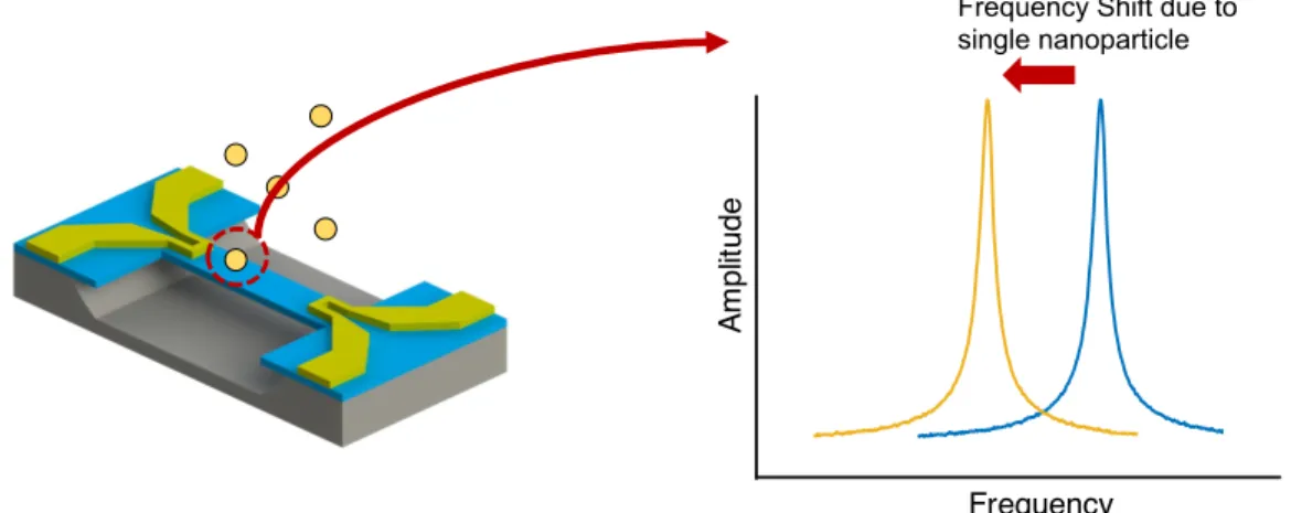
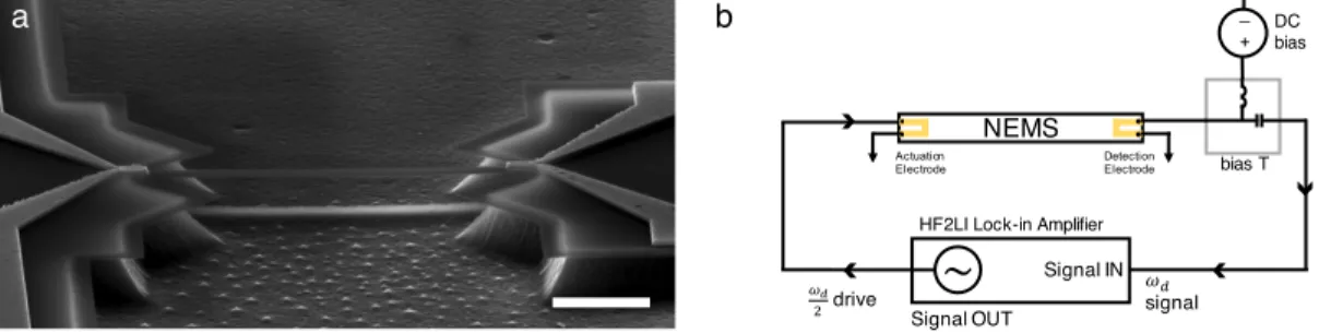
Single nanoparticle sensing with nanoelectromechanical resonators operating at nonlinear regime

2) Second, in the QDBC approach, a data block is assumed to be private from the beginning of program execution and stays private as long as the corresponding subpage is accessed by

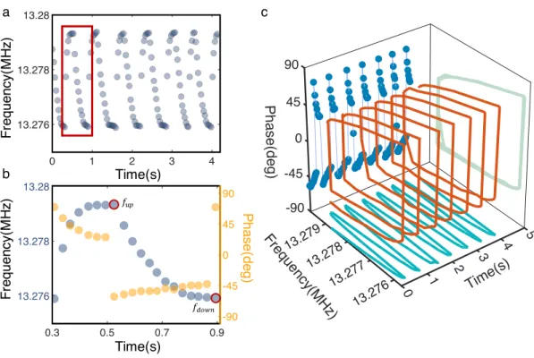
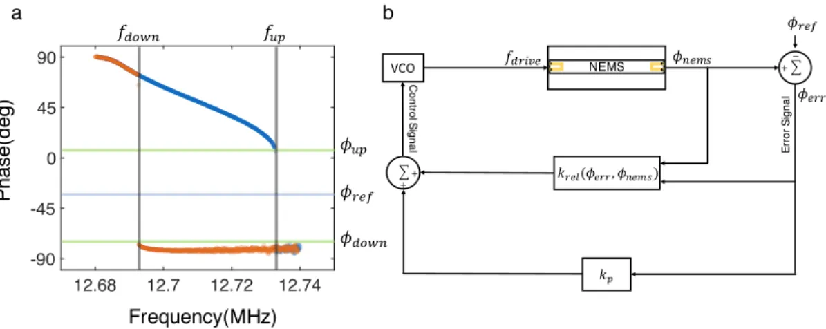
So, the tetragonal based me- tallic defect structures were found to be superior to fct based metallic defect structures in terms of peak amplitude and the maximum achievable Q

In mixtures containing halogens (gaseous dielectrics) most of the electrons are slowed down or replaced by the heavier negative fragment ions hence production of

Before turning to questions about the relationship of money to the economy, princi- pally its impact in determining prices and its role in commercialization, it seems best to start

Our theory reveals two different mechanisms driving the like-charge polyelectrolyte-membrane complexation: In weakly charged membranes, repulsive polyelectrolyte-membrane

The main aim of this study is to examine predictive validity of a laboratory high school admission examination using several exit variables such as international and national

Havaciva kökünden elde edilen, kırmızı ve mavi bileşenle boyanan keten ve pamuk kumaş numuneler için haslık analiz sonuçlarının ortalaması ve bu haslık

The following were emphasized as requirements when teaching robotics to children: (1) it is possible to have children collaborate in the process of robotics design, (2) attention