A Finite Concave Minimization Algorithm Using
Branch and Bound and Neighbor Generation
H A R O L D P. B E N S O N and S E R P I L S A Y I N *Department of Decision and Information Sciences, University of Florida, Gainesville, FL 32611-2017, U.S.A.
(Received: 21 May 1992; accepted: 18 October 1993)
Abstract. In this article we present a new finite algorithm for globally minimizing a concave function over a compact polyhedron. The algorithm combines a branch and bound search with a new process called neighbor generation. It is guaranteed to find an exact, extreme point optimal solution, does not require the objective function to be separable or even analytically defined, requires no nonlinear computations, and requires no determinations of convex envelopes or underestimating functions. Linear programs are solved in the branch and bound search which do not grow in size and differ from one another in only one column of data. Some preliminary computational experience is also presented.
Key words. Concave minimization, branch and bound, global optimization.
I. Introduction
The purpose of this article is to present a new algorithm for solving the concave minimization problem (P) given by
min
f(x),
subject to x E X ,where X is a nonempty, compact polyhedral set in R n, and f is a real-valued concave function on some open set Y in R n that contains X. Problem (P) may have many locally optimal solutions which are not globally optimal, so that it represents a type of
global optimization
problem [8]. However, it is well known that there exists an extreme point of X which is a globally optimal solution of problem (P). Let m denote the optimal objective function value of problem (P).Problem (P) has been the subject of intense interest for almost 30 years. There are at least two reasons for this. First; large classes of important decision models arising from a variety of applications lead to formulations involving the minimiza- tion of concave functions over polyhedra. Included in these applications are various problems involving economies of scale, production planning, and en- gineering design, to name a few. Second, many optimization problems which originally are not concave can be transformed into equivalent concave minimiza- tions over polyhedra, including zero-one integer programming problems, bilinear programming problems, fixed charge problems, and linear complementarity problems. Surveys of the applications and importance of problem (P) can be
* Current affiliation: Management Department, Bilkent University, Ankara, Turkey.
Journal of Global Optimization 5: 1-14, 1994.
2 H.P. BENSON AND S. SAYIN
found, for instance, in Pardalos and Rosen [14, 15], Horst [6], and Horst and Tuy [8].
From the viewpoint of computational complexity, the concave minimization problem (P) is NP-hard, even in the special case of minimizing a quadratic concave function over a very simple polyhedron such as a hypercube [16]. However, complexity results of this nature characterize worst-case instances. Hence the search for more practical algorithms for globally solving problem (P) remains an important undertaking.
Current methods for solving problem (P) usually use either cutting planes, extreme point ranking, inner approximation, outer approximation, branch and bound, or a combination of these approaches. A survey of the algorithms available for solving problem (P) will not be given here. Instead, the reader is referred to McCormick [11], Heising-Goodman [3], Rosen [18], Horst [5], Benson [1], Pardalos and Rosen [14, 15], Horst [6], and Horst and Tuy [8] for com- prehensive discussions of these algorithms.
In this article we present a finite algorithm for solving the concave minimization problem (P). The algorithm finds a globally optimal extreme point solution for problem (P) by combining a branch and bound search with a neighbor generation process. The neighbor generation process helps to generate incumbent solutions and to ensure that the algorithm is implementable and convergent. In addition, the algorithm has the following advantages:
(i) It finds an exact, extreme point optimal solution.
(ii) It does not require f to be separable or even analytically defined.
(iii) It requires no nonlinear computations and no determinations of convex envelopes or other underestimating functions.
(iv) It solves linear programming problems in the branch and bound search which do not grow in size and differ from one another in only one column of data. (v) It avoids solving some linear programs through the use of a fathoming
procedure.
Part of the motivation for developing the algorithm comes from previous work by Soland [19], Horst [4], and Benson [1]. The algorithm is similar in certain respects to the algorithms presented in these papers. However, important differences exist. Furthermore, the convergence of the algorithm given here is guaranteed in a different way. Therefore, we will present the algorithm in its entirety without assuming any knowledge of these algorithms.
The plan of this article is as follows. In Section 2 certain theoretical pre- requisites needed for developing the algorithm are presented. In Section 3 the new algorithm for solving problem (P) is presented, its convergence properties are shown, and its computational benefits are reviewed. Some preliminary computational experience with the algorithm is reported in the final section.
2. Theoretical Prerequisites
BRANCH AND BOUND AND NEIGHBOR GENERATION 3 where A is a p x n matrix and b ~ R p. We shall also assume familiarity with certain basic concepts commonly used in global optimization, including the notions of an n-dimensional simplex (or, more briefly, an n-simplex) a vertex of an n-simplex, a partition of a subset of R n, a radial subdivision of an n-simplex, and the convex envelope of a lower semicontinuous function on a compact convex subset of R n. Definitions and discussions of these concepts can be found, for instance, in [8].
One of the key procedures used in the algorithm to be presented for problem (P) involves computing a lower bound for f over S A X for an arbitrary n-simplex S. To compute this lower bound, the algorithm finds an extreme point of X which minimizes the convex envelope fs of f on S over X. It is well known (cf. [4, 8]) that fs is affine over both S and R n, and that it can be found by solving a system of linear equations. However, the algorithm to be given finds the minimum of fs over X and an extreme point of X which achieves this minimum without requiring the explicit determination of the function fs. To achieve this, it relies upon the following result.
T H E O R E M 1. Let S C_ Y be an n-simplex with vertices v ~ v 1 , . . , , V n, and let
fs: Rn---> R be the convex envelope o f f on S. Consider the linear program (Ix) given by
min fs(X) , subject to x E X , and the linear program (Px) given by
min ~ f(vi)Ai , i=O subject to ~ (Avi)Ai <= b , i = 0 ~ A i = l . i = 0
Let A denote the feasible region for the linear program (P~).
(i) f f ,( E A, then ~ = Eino fti vi belongs to X and fs(~ ) = Ein0 f(vi)Ai. Converse- ly, if ~ E X , then there exists a unique A E A such that ~=Zinofti vi which, furthermore, satisfies fs (fc) = E in-_ o f(vi) Ai.
(ii) If A is an extreme point of A, then ~ = Ein0 fti vi is an extreme point of X. Conversely, if fc is an extreme point of X, then the unique ~ ~ A such that .~ = Hi= 0 Air is an extreme point of A.
(iii) The optimal values of the linear programs (Px) and (P~) are equal. If A* is an optimal solution for problem (Pa), then x* = Z in o A* v i is an optimal solution for problem (Px). I f x* is an optimal solution for problem (Px), then the unique A* ~ A such that x* -- E/no A*v ~ is an optimal solution for problem (Pa).
Proof. (i) Assume that A C A . Let ~ = Ein0 Air/. Since Zin0 (Avi)fti <- b, the definition of ~ implies that A ~ _-<b, i.e., ~ E X. From [4, 8], fs is an affine
H . P . B E N S O N A N D S . S A Y I N
function and satisfies fs(V ~) =f(v~), i = O, 1 , . . . , n. Therefore, from the definition
n ^ i n ^ i n
of
2, fs(2) =fs(Zi=o hiv
) = Ei= 0 hffs(V ) = E/= 0 hif(vg).To show the converse statement in (i), assume that 2 E X. Since S is an n-simplex, the vectors
v i, i--O, 1 , . . . , n,
are affinely independent. For each i = 0, 1 , . . . , n, form the vector w g E R "+1 whose first n entries equal those of v ~ and whose ( n + 1)st entry is one. Thenw i,
i = 0 , 1 , . . .,n
are linearly in- dependent vectors in R n+l. Therefore, they form a basis for R n+l. Let )3 E R n~l denote the vector whose first n entries equal those of 2 and whose (n + 1)st entry is one. Then, since 33 E R "+a, there exists aunique
h ~ R n+l such that 33 =n ^ i ^ n ^ i n
Eg= 0 h~w. This implies that x = E~= 0 h~v and Ei= 0 '~i = 1. Furthermore, since
2 E X, Ei~ o (Av!)~ i = A
ET= 0 hi vi= A 2 <= b: Therefore, h E A. Finally, since fs isaffine and satisfies fs(V i) =f(vi), i = 0, 1 , . . . , n, we obtain fs(YC) = fs(Ei"=0 hi vi) =
n ^ i n
Ei=0 hffs(V ) = Z,= 0 hff(vi).
n ^ i
(ii) Assume that h is an extreme point of A. Let 2 = 2~=0 h~v. Then, by part (i), 2 ~ X. Since 2 E X, again using part (i), it follows that no ~ ~ A, ~ ~ A, exists such that 2 = Ei~o h~ v~.
Suppose that 2 is not an extreme point of X. Then, since 2 ~ X , for some points x 1,
x 2 ~ X
distinct from s and for some 0 ~ ( 0 , 1),2 =Oxa+
( 1 - O ) x 2.X 2 ~ n
Since x ~, ~ X, by part (i), for each ] = 1, 2, x ] 21=o
"~ vi
for some h 1, h e ~ A. Therefore,=0 21~:vi"[-(1--O) ~ t~2V i
/ = 0 i = 0= s [Oh[ +(1-O)h2ilv i
i = 0 = s [0h' + (1 -O)h2]i vi ,
i = 0where, by convexity of A, [0,~1 + ( 1 - 0)~ 2] E A. Since no h ~ A , h # A, exists
n - i
such that 2 = Ei= 0 h~v, this implies that h = 0h x + (1 - 0),~ 2. Therefore, h = ,~a = h 2, since h is an extreme point of A. On the other hand, since x j ~ 2, j = 1, 2, h! ~ ~, ] = 1, 2. This contradictioh implies that the assumption that 2 is not an extreme point of X must be false.
To show the converse statement in (ii), assume that 2 is an extreme point of X. Let A be the unique element of A which satisfies 2 = E ~ o hiv ~.
Suppose that h is not an extreme point of A. Then, since ,~ E A, for some points
/ ~ 1 , / ~ 2 ~ A distinct from ,~ and for some 0 E (0, 1), h = 0/~ 1 -~ (1 - 0)/~ 2. Then
n
fc = i = 0
= 2 [0~ 1 + ( 1 - O ) h 2 ] i v i
i=O
B R A N C H A N D B O U N D A N D N E I G H B O R G E N E R A T I O N 5
:0 ~ A~vi-C (1--O) ~ A2iv i
i = 0 i=O
= Ox 1 + (1 - O ) x 2 ,
where, for each j = 1, 2, x j = Y'/C0 A{ vi. By part (i), x j ~ X , j = 1, 2. Also, since
n ^ i x j
A j ~ A, j = 1, 2, and A is the unique element of A satisfying 2 = r,~=0 Air, ~ 2, j = 1, 2. On the other hand, since 2 is an extreme point of X and 2 = Ox I + (1 -
0)x 2, 2 = x 1= x 2. This contradiction implies that the assumption that A is not an extreme point of A is untenable, and the proof of part (ii) is complete.
(iii) Assume that A* is an optimal solution for problem (PA). Let x * = n , i
Zi= 0 A iv , and let Y be an arbitrary element of X. Then, by part (i), x* E X and, for some unique A E A, 2 = Zi~=o X,.v i. Since A* is an optimal solution for problem (in,),
i = 0 i = 0
F r o m part (i), fs(X*) : E~=0 n f(vi)A, andfs(X- ) = , Z i = 0 f ( o i - )1~ i . Therefore, from (1),
fs(X*) <=fs(~. This implies that x* is an optimal solution for problem (Px). Also, since fs(X*)= E/"=0 f(vi)M], the optimal values of problems (Px) and (P,) are equal.
Assume that x* is an optimal solution for problem (Px). Let A*E A be the
n , i
unique element of A satisfying x* = E i= 0 A i r . Let X be an arbitrary element of A. Then, by part (i), 2 = Ei~ 0 A-~v i belongs to X. Since x* is an optimal solution for problem (P~), this implies that fs(x*) _-<fs(X-). From part (i), fs(X*) = Zi= 0 " f(vi)Ai*
n n n
and fs(2) = Zi= 0 f(vi)Ai. Therefore, Zi= 0 f(vi)A * <-_ r.i= 0 f(vi)Xi . This implies that A* is an optimal solution for problem (P~), and the proof is complete.
Notice from Theorem 1 that to solve the linear program (Px), the linear program (P~) can be solved instead. In particular, the optimal value of problem (P~) equals the optimal value of problem (Px), and for any optimal extreme point solution A * E A for problem (PA), x*=[Ei"=oA*Vi] E X is an optimal extreme point solution for problem (Px). The algorithm will make repeated use of these facts to find lower bounds and extreme points of X which achieve these lower bounds.
3. The Algorithm
3.1. A L G O R I T H M STATEMENT
In each step k of the algorithm, a global lower bound LB k for m is found via branch and bound. To accomplish this, first an initial n-simplex S O is chosen that contains X and is a subset of Y. Then, in a typical step k, a radial subdivision of a sub-n-simplex S k-I of S O is performed. This yields a partition T k of S k-1 and a
6 H . P . BENSON AND S. SAYIN
new partition
Qk
of S O of the formQk
=
(ak-l\sk-I)
I.J T k,
whereQk-1
is the partition of S O obtained from step k - 1. The partitionQk
of S O consists of a set of n-simplices d e n o t e d{S j I J E I(Qk)},
whereI(Q k)
is a finite index set. For each n-simplex S j inQk
that does not belong toT k,
a lower bound wj. for the minimum of f over S j f3 X is available from some previous step. For each n-simplex S j inQk
that belongs toT k,
a lower bound wj for the minimum of f over S j fq X is c o m p u t e d in step k. W h e t h e r or not the value of wj. is c o m p u t e d prior to or during step k, a linear programming problem of the form (PA) (see T h e o r e m 1) is solved to help c o m p u t e it. T o find the global lower bound LB k for m, the algorithm computes the minimum wj of the valueswj, j E I(Qk),
and sets LB k = wj.T h e neighbor generation process used in the algorithm helps primarily to ensure that the algorithm is implementable and convergent. As a by-product, however, it helps to generate incumbent solutions.
T h e neighbor generation process is invoked in a typical step whenever an e x t r e m e point of X is found which will serve or is being considered for serving as the basis of a radial subdivision of some sub-n-simplex in the next step. When such an extreme point x is found, the neighbor generation process is invoked to search among all of the neighboring extreme points of x in X for those which have not yet served as vertices of any sub-n-simplex of S O created thus far in the algorithm, z~ '" . L is maintained throughout the algorithm which, at any given time, stores all e x t r e m e points of X found via the neighbor generation process which have not yet served as vertices of a sub-n-simplex of S O thus far created by the algorithm.
In a typical step k, the extreme point
x]
of X found from solving the linear p r o g r a m (Px) that was solved to help compute LB k =w]
is used as the basis of the next radial subdivision in the next step. H o w e v e r , if xj has already served as a vertex of some sub-n-simplex of S ~ the algorithm examines the list L. If L -- 0, the algorithm terminates since, as we shall see ( T h e o r e m 2), this guarantees that all e x t r e m e points of X have been found. If L ~ 0 , elements Y of L are individually r e m o v e d from L until one is found, if possible, which can serve as the basis of the n e x t radial subdivision. T o qualify for this, 2 must fail a fathoming test. In this way, each step k either finds an extreme point of X for use in a radial subdivision in the next step, or, failing to do so, terminates with L = 0.W h e n the algorithm must r e m o v e points from L for
consideration for use
as the basis of a radial subdivision, the neighbor generation process is invoked for each such point. T h e neighbor generation process is also invoked whenever an extreme point of X is successfully found foractual
use in the next radial subdivision, regardless of whether it was found from computing LB k or from the list L.As linear programs of the form (P~) are solved and as the neighbor generation process is invoked, the algorithm identifies various extreme point feasible solutions of problem (P). Each step k computes an upper bound U B k for m given by the minimum objective function value in problem (P) of all such points thus far e n c o u n t e r e d . T h r o u g h o u t the algorithm, for each k, a record is kept of an
BRANCH AND BOUND AND NEIGHBOR GENERATION 7
e x t r e m e point x c of X (the i n c u m b e n t solution) which satisfies f ( x c) = UB k . Thus, as a by-product of the neighbor generation process, incumbent solutions may be f o u n d which might not otherwise have been detected. W h e n e v e r LBg = U B k , the algorithm terminates.
We may now give a formal statement of the algorithm. In the algorithm statement, V L is a list maintained by the algorithm which, at any given time, stores all points that have served or have been considered for serving as a vertex of a subsimplex of S O created by the algorithm.
Step 0
0.1. Choose an n-simplex sO___ Y such that XC_ S O and let Q 0 = {sO}. Let the vertices of S~ be {v ~ v 1, . , v n } . S e t N = O a n d V L = { v ~ . . . . . 1, , v"}, For each i E {0, 1 . . . . , n} for which v i ~ X , set N = N U {v i} and generate the set E i of e x t r e m e points of X adjacent to v i in X which do not belong to VL. For each i ~ {0, 1 , . . . , n } for which v i ~ X , set Ei =t~. Set L = u / n 0 E i. If N = ~ , set U B = + ~ and go to step 0.2. If N # 0, choose x C E a r g m i n { f ( x ) Ix E N U L} and set U B =f(xC).
0.2. Find the optimal value q0 and an extreme point optimal solution h * E A
n , i
for the linear program (Px) (see T h e o r e m 1). Let x* = E~= 0 hi v , set w 0 = q0, and set 2-0 = x*. G e n e r a t e the set E of extreme points of X adjacent to 2-~ which do not belong to VL. If E C _ L , go to S t e p 0.3. Otherwise, set L = L U E and continue.
0.3. Set LB 0 = w 0. Set UB 0 = min{UB, {f(x) Ix ~ {k -~ LJ E}}. If U B ~ + ~, choose 2 ~ argmin{f(x~), { f ( x ) I x E {2 -~ U E}} and set x c = 2. Otherwise, choose 2 ~ argmin{f(x) Ix ~ {2 ~ U E} and set x ~ = 2. If LB o = U B 0 , conclude that x c is an optimal solution for problem (P) and stop. Otherwise, set k = 1 and go to step k.
Step k, k --- 1. A t the beginning of step k, a partition Q~-I of S O is available f r o m the previous step. Also available for each n-simplex S j E Qk-X are a lower b o u n d wj for the minimum o f f over S j C) X and an extreme point x j E X found in the process of computing this lower bound. Assume that S k-1 ~ Q~-~ denotes an e l e m e n t of Qk-a which contains the point 2 k-1 computed in the previous step.
k.1. If s (~ L, r e m o v e s from L. Using 2 k-1 ~ S k-1 as a basis, p e r f o r m a radial subdivision of S k-1 to obtain a partition T ~ of S k-1. Set V L = V L U {s
k.2. F o r each n-simplex S j E T k :
(i) With v ~, i = 0, 1 , . . . , n set equal to the vertices of S j, find the optimal value qj and an e x t r e m e point optimal solution h* E A for the linear program (P,) (see T h e o r e m 1);
n , i
(ii) Set x i = E~= 0 A i r ; and (iii) Set w i = m a x { q j , Wk_x}.
k.3. Set U B k = min{UBk_a, {f(x j) [S j E Tk}}. If U B k = f ( x j) for some j such that S j E T k, set x ~ = x j.
8 H . P . B E N S O N A N D S. S A Y I N
k.5. L e t w; = min{wj [ j E I(Qk)), and set LB k = w].
k.6. If LB k = U B k , conclude that x c is an optimal solution for problem (P) and stop. Otherwise, continue.
k.7. (i) If x]ff.VL, set s =X ] and go to step k.8. Otherwise, continue. (ii) If L = 0, conclude, that x c is an optimal solution for problem (P) and stop. Otherwise, remove any point ~ from L and continue.
(iii) Find any n-simplex S i E Qk which contains s If wj _---UBk, set s = s and go to step k.8. Otherwise, continue.
(iv) G e n e r a t e the set E of extreme points of X adjacent to E which do not belong to VL. Set V L = V L U {s If E _C L, go to step k. 7(ii). Otherwise, set L = L U E , find 2 E argmin{f(x~), {f(x) [x E E}}, set x c = 2, set U B k = f(xC), and go to step k. 7(ii).
k.8. G e n e r a t e the set E of extreme points of X adjacent to s which do not belong t o V L . If E C L, set k = k + 1 and go to step k. Otherwise, set L = L U E, find 2 ~ argmin{f(xC), {f(x) [x E E}}, set x ~ = 2, set U B k ---f(xC), set k = k + 1, and go to step k.
T h e set N in step 0.1 stores each vertex v i of S O which is also an extreme point of X. Since S O D X, it is easily shown that for any vertex v i of S ~ if v i E X, then v i is an e x t r e m e point of X. Step 0.1 relies on this fact to construct N.
In step k. 7(iii), if the lower bound w i for the simplex S f containing the point s r e m o v e d from L exceeds UBk, then control is passed to step k.7(iv). In step k. 7(iv), the usual neighbor generation process for s and the associated incumbent u p d a t e are p e r f o r m e d , and s is added to the list VL. H o w e v e r , control then passes to step k. 7(ii) rather than to step k + 1. In particular, no radial subdivision of the simplex S i is p e r f o r m e d , and no linear programming problems Of the form (Px) that would be associated with this radial subdivision are solved. In this sense, the simplex S i is fathomed. Notice that the point s is not used at this stage as a basis of a radial subdivision in the next step. H o w e v e r , since it was a candidate for such a use, s is added to the set VL.
3.2. C O N V E R G E N C E
We will now show that the algorithm finds an optimal extreme point solution for p r o b l e m (P) in a finite n u m b e r of steps. T o show this, the following result is needed.
T H E O R E M 2. For any k >- 1, if L = 0 in step k. 7(ii) of the algorithm, then V L contains every extreme point of X.
Proof. Assume that k _-__ 1. T o prove the t h e o r e m , we will prove the contraposi- tive. T h e r e f o r e , assume at step k.7(ii) that an extreme point 2 E X exists which does not belong to VL. T h e n either (1) at least one extreme point of X adjacent to 2 belongs to V L or (2) no extreme point of X adjacent to 2 belongs to VL.
BRANCH AND BOUND AND NEIGHBOR GENERATION 9
extreme point y of X added to V L through step k. 7(ii) of the algorithm, from steps 0.1 and 0.2 and from steps w.1, w.7, and w.8,
l<=w<-k,
the neighbor generation process guarantees that all extreme points of X adjacent to y which do not belong to VL are contained in L. Since x is an extreme point of X adjacent to $ which belongs to V L in step k. 7(ii), and 2 ~ VL, this implies that $ E L. Hence, in this case, L r 0.Case 2.
No extreme point of X adjacent to 2 belongs to VL. Consider theextreme point y0 E X. From step 1.1, y0 E VL. Since X is a polyhedron, there exist a finite number of extreme points y l y 2 , . . . , yt of X such that 2 is adjacent to y l , yh is adjacent to yh+X for each h = 1, 2 , . . . , t - 1, and yt is adjacent to E ~ Let Y = {y E {yl, y2 . . . . , y t } l y ~ . V L }. Since yl is adjacent to 2 and no extreme point of X adjacent to 2 belongs to VL, ya ~ V L . Therefore, I r 0 and we may choose an integer h* such that
h* = m a x { h E {1,2 . . . . , t } l y h ~ V L } .
If h * < t, then
yh*
is adjacent to yh*+l E WE. If h * = t, thenyh*
is adjacent to 2-0 E VL. In either case,yh* is an extreme point of X which does not belong to VL
but which is adjacent to an extreme point of X whichdoes
belong to VL. Then, by the same reasoning as used in Case 1 for 2, it follows thatyh* ~ L.
Since this implies that L r 0, the proof is complete.We may now show the following result.
T H E O R E M 3.
Whenever the algorithm terminates, the algorithm's current incum-
bent solution x c is an extreme point optimal solution for problem (P).
Proof.
Consider any stepk, k >= O,
of the algorithm. From step 0.3 or, fork = 1, from step
k.5,
LB k = min{wj I J E / ( O h ) } . (2)
For each j E I(Qk), by Theorem 1, qj, calculated in step k.2(i) for some k =< k, is a lower bound for the minimum o f f over X A S j. In addition, for any sets A and B such that A 7 B, any lower bound for the minimum of f over B is a lower b o u n d for the minimum o f f over A. The latter two statements imply that for each
j E I(Qk), wj,
calculated in step k.2(iii) for some k _--<k,
is a lower bound for theminimum mj of f over X fq S J. Therefore,
min{wj I J E i(Qk)} < min {mj t J E I(Qk)}. (3)
The set {Sil j E I ( Q k ) } is a partition of S O D X . This implies that the right-hand- side of inequality (3) is identical to m. From (2), this implies that LB k =< m.
Suppose that the algorithm terminates in step k. Then either (1) LB k = UB~ or (2) L = ~.
10 H. P. B E N S O N A N D S. SAYIN
extreme point solution, it follows that in this case, L B k = f ( x C ) . From the discussion above, LB k =< m. Therefore, f ( x c) <= m. Since x ~ E X , this implies that f ( x ~) = m, so that x c is an extreme point optimal solution for problem (P).
Case 2. L = 0. Then k => 1, the algorithm terminates in step k. 7(ii), and, from Theorem 2, VL contains every extreme point of X. From steps 0.1, 0.3 and steps k.1, k.3, k.7, and ft.8, 1 <= fc <- k, for any extreme point :~ of X contained inVL by step k.7, UBk<=f(2). Since U B k = f ( x C ) , where x c is the current incumbent extreme point solution, and since VL contains every extreme point of X, this implies that f ( x ~) <=f(x) for all extreme points x of X. Since problem (P) has an optimal solution which is an extreme point of X, it follows that x c is an extreme point optimal solution for problem (P), and the proof is complete.
The algorithm always eventually terminates by the following result. T H E O R E M 4. The algorithm terminates in a finite number o f steps.
Proof. Suppose, to the contrary, that the algorithm does not terminate in a finite number of steps. Then step k.7 is executed an infinite number of times. Therefore, in an infinite number of executions of step k.7, either (1) the point x j in step k. 7(i) does not lie in VL, or (2) a point s in step k. 7(ii) is removed from L.
Case 1. In an infinite number of executions of step k. 7, x ] in step k. 7(i) does not lie in VL. From steps k.1 and k.7(i), whenever x ] N V L in some step, it is added to the set VL in the next step. But each point x ] is an extreme point of X, and X contains a finite number of extreme points. The latter two statements imply that it is impossible for x j not to belong to VL in an infinite number of executions of step k. 7(i). Therefore, this case cannot occur.
Case 2. In an infinite number of executions of step k. 7, a point s in step k.7(ii) is removed from L. From steps 0.1, 0.2, k . 7 and k.8, L contains only extreme points of X, and the only points ever added to L by the algorithm are extreme points of X not already contained in L. Since X contains a finite number of extreme points, this implies that it is impossible to execute the removal of a point in step k. 7(ii) from L an infinite number of times. Therefore, this case cannot
o c c u r .
It follows that the assumption that the algorithm does not terminate in a finite number of steps is false, and the proof is complete.
Taken together, Theorems 3 and 4 imply that the algorithm is guaranteed to find an optimal solution for problem (P) in a finite number of steps. Furthermore, the optimal solution that it finds is an extreme point of X.
3.3. COMPUTATIONAL BENEFITS
The branch and bound-neighbor generation algorithm that we have presented for problem (P) has several attractive computational benefits.
B R A N C H A N D B O U N D A N D N E I G H B O R G E N E R A T I O N l l
First, as shown in Section 3.2, it is guaranteed to find an exact, extreme point optimal solution for problem (P) in a finite number of steps.
Second, it does not require f to be separable or even analytically defined. The only requirement for f is that it be a real-valued concave function on some open set Y in R n that contains X.
Third, the algorithm requires no nonlinear computations and no determinations of convex envelopes or other underestimating functions.
Fourth, the linear programming problems solved during the branch and bound search do not grow in size and differ from one another in only one column of data. In particular, these linear programs are all of the form of problem (P~) given in Theorem 1. Thus, they all contain (p + 1) constraints and (n + 1) variables. Furthermore, for each n-simplex S j E T k in step k . 2 , the vertices of S j
are identical to those of its parent n-simplex S ~-1, except that in S j the vertex
- k - 1
x replaces one of the vertices v i of S k-1 As a result, the linear program (P,) associated with S j which is solved in step k . 2 differs from the one solved earlier for S k-~ only in the (p + 1) coefficients for A i in the objective function and in the first p constraints. This implies that if the simplex method is used, for instance, to solve the linear programs (Pz), the optimal basis found previously for the linear program (P~) associated with S ~-a can be used as a starting basis for the simplex method solution of the problem (P~) associated with S j. In this way, the linear programs (P,) can, in general, be more quickly solved than they would be by using the traditional Phase I-Phase II approach of the simplex method [13].
Fifth, the algorithm incorporates a fathoming procedure to save unnecessary computations. In particular, in step k. 7(iii), if wf > UBk, the simplex S I is not partitioned and no linear programs of the form (P~) that would be associated with this partitioning process are solved.
The algorithm has other advantages. For instance, at each step of the algorithm, an incumbent extreme point solution x c of X is available. This incumbent solution, while not necessarily an optimal solution, may often provide a user of the algorithm with a very good feasible solution for problem (P) when the number of steps executed grows large and the algorithm must therefore be prematurely terminated. In particular, the neighbor generation process can be expected to enhance the quality of this incumbent solution.
4. Preliminary Computational Experience
We have written a computer code in C which implements the proposed algorithm. We constructed 60 test problems, and used the code to solve these problems on an IBM 3090 Model 600J mainframe computer. In this section, we describe the code, the sources of the test problems, and the computational effort that the code required to solve the problems.
It has been pointed out [2, 7, 15] that the difficulty of finding a globally optimal solution to a concave minimization problem limits the sizes of problems solvable
12 H . P . B E N S O N A N D S. S A Y I N
by reasonable effort. Furthermore, the amount of reported information about the computational behavior of existing algorithms is limited. Since there are not generally-accepted test problems, we have constructed various test problems partially based on some data in the literature. Our goals in constructing and solving these test problems are limited. We merely sought to make some preliminary conclusions about the algorithm.
The code uses the simplex-based subroutines of the Optimization Subroutine Library [9] to solve the linear programming problems (P~) called for in the algorithm. In each run, the initial simplex S O that contains X was constructed separately using a method proposed by Horst [4]. The linear programming problems required by Horst's method are also solved by the simplex method procedures given in the subroutines of the Optimization Subroutine Library [9]. The branch and bound tree and the lists L and VL were maintained and processed using dynamic data structures.
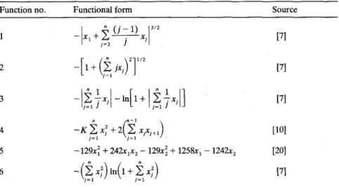
The test problems were constructed as follows. Using data from Pegden and Petersen [17], we constructed eight nonempty, compact polyhedra of five different sizes. Each size is defined by the number of rows (m) and the number of columns (n) in the matrix B, where X = {x E R n I B x <= g, x >= 0}, and g ~ R m. Next, we obtained six different types of concave functions from the literature to use as objective functions. The forms and sources of these functions are given in Table I. In function number 4, K represents any positive integer. We also obtained some variations of these functions by appending linear terms, negative quadratic terms, or both. Last, we combined the compact polyhedra with the concave functions in various combinations to create five categories of 12 problems each, where a category of problems is defined by the common size (m, n) of the feasible regions of the problems in the category.
Table I. Some objective function forms
Function no. Functional form Source
- - X l n ( j _ 1) X 3/2 1 + j~----f--- j [7] 2 - [1 + (j~l jx/)2] 1/z [71 3 - , ~ 1 1 x , - I n [ l + , ~ i x , ] [71 n n - - 1
4
- K ~ x ~ +
2(~'~xjxj+l)
[101 j = l - i = 1 " ' 5 - 1 2 9 x 2 + 242xlx z - 129x~ + 1258x~ - 1242x 2 [20]( " : ) ( " )
6 - E x In l+Y~x~ [71 - j = l - - j = lBRANCH AND BOUND AND NEIGHBOR GENERATION 13
Table II. Computational results: averages Category
m n Iterations Nodes Pivots Pseudo-pivots CPU time
4 5 13.08 44.08 89.83 82.50 1.94
8 6 6.67 20.75 42.92 100.50 1.83
3 7 0.42 2.00 10.08 24.50 1.58
3 8 0.50 2.42 10.25 28.70 1.57
5 10 10.25 42.83 97.58 330.80 2.42
F o r simplicity, we solved only problems in which each extreme point of X that was e n c o u n t e r e d was nondegenerate. This shortened the code required to execute the neighbor generation process. This part of the code uses simplex-type pivots, which we call pseudo-pivots. A l t h o u g h the degenerate case can be handled by pseudo-pivots as well, the process in this case can become rather complicated [12, 13]. F o r this reason, in these initial computational experiments, we decided to eliminate the problems in which degenerate extreme points were encountered. F o r each solved problem, the c o m p u t e r code was executed until either an incumbent solution was found with an objective function value guaranteed to be within five percent of the optimal objective function value, or until the list L b e c a m e empty.
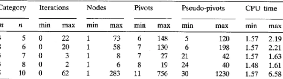
Statistics summarizing the results of our computations are given in Tables II and III. In each table, five measures are used to evaluate the results: N u m b e r of iterations of the algorithm, n u m b e r of nodes created in the branch and b o u n d search (which equals the n u m b e r of linear programs (P~) solved), total n u m b e r of simplex m e t h o d pivots required to solve the problems (Px), n u m b e r of simplex- type pseudo-pivots, and the C P U time in seconds. Table II gives the averages of these measures by category. In Table III, the minimum and the maximum for each measure in each category are reported.
F r o m Table II, we see that the computational effort required to solve these 60 p r o b l e m s does not necessarily monotonically increase as m or n increases. Also, f r o m Table III, we note that the variance in the computational effort needed to solve the problems within a category can be relatively small or relatively large. These two observations seem to suggest that structural factors other than problem size significantly contributed to the computational effort required to solve these 60
Table III. Computational results: extremes
Category Iterations Nodes P i v o t s Pseudo-pivots CPU time
m n min max min max min max min max min max
4 5 0 22 1 73 6 148 5 120 1.57 2.19
8 6 0 20 1 58 7 130 6 198 1.57 2.21
3 7 0 3 1 8 7 27 21 42 1.57 1.63
3 8 0 2 1 6 8 19 24 40 1.48 1.61
14 H. P. B E N S O N A N D S. S A Y I N
problems. This is consistent with preliminary results obtained for other types of global optimization problems (see, e.g., [2, 7]).
Although the code successfully solved each of the 60 test problems, we cannot as yet draw any conclusions concerning its practicality for larger problems. More computational testing will be required to investigate this issue.
References
1. Benson, H. P. (1985), A Finite Algorithm for Concave Minimization over a Polyhedron, Naval
Research Logistics Quarterly 32, 165-177.
2. Benson, H. P. and Erenguc, S. S. (1990), An Algorithm for Concave Integer Minimization over a
Polyhedron, Naval Research Logistics 37, 515-525.
3. Heising-Goodman, C. D. (1981), A Survey of Methodology for the Global Minimization of
Concave Functions Subject to Convex Constraints, Omega 9, 313-319.
4. Horst, R. (1976), An Algorithm for Nonconvex Programming Problems, Mathematical Program-
ming 10, 312-321.
5. Horst, R. (1984), On the Global Minimization of Concave Functions: Introduction and Survey,
Operations Research Spektrum 6, 195-205.
6. Horst R. (1990), Deterministic Methods in Constrained Global Optimization: Some Recent
Advances and New Fields of Application, Naval Research Logistics 37, 433-471.
7. Horst, R . , Thoai, N. V., and Benson, H. P. (1991), Concave Minimization via Conical Partitions
and Polyhedral Outer Approximation, Mathematical Programming 50, 259-274.
8. Horst, R. and Tuy, H. (1993), Global Optimization (Deterministic Approaches), 2nd Edition,
Springer, Berlin.
9. International Business Machines (1990), Optimization Subroutine Library Guide and Reference,
International Business Machines, Mechanicsburg, Pennsylvania.
10. Konno, H. (1976), Maximization of a Convex Quadratic Function Subject to Linear Constraints,
Mathematical Programming 11, 117-127.
11. McCormick, G. P. (1972), Attempts to Calculate Global Solutions of Problems that may have
Local Minima, in F. Lootsma (ed.), Numerical Methods for Nonlinear Optimization, Academic
Press, London, 209-221.
12. Murty, K. G. (1968), Solving the Fixed Charge Problem by Ranking the Extreme Points,
Operations Research 16, 268-279.
13. Murty, K. G. (1983), Linear Programming, Wiley, New York.
14. Parda!os, P. M. and Rosen, J. B. (1986), Methods for Global Concave Minimization: A
Bibliographic Survey, SIAM Review 28, 367-379.
15. Pardalos, P. M. and Rosen, J. B. (1987), Constrained Global Optimization: Algorithms and
Applications, Springer, Bedim
16. Pardalos, P. M. and Schnitger, G. (1987), Checking Local Optimality in Constrained Quadratic
Programming is NP-Hard, Operations Research Letters 7, 33-35.
17. Pegden, C. D. and Petersen, C. C. (1979), An Algorithm (GIPC2) for Solving Integer
Programming Problems with Separable Nonlinear Objective Functions, Naval Research Logistics
Quarterly 26, 595-609.
18. Rosen, J. B. (1983), Global Minimization of a Linearly Constrained Concave Function by
Partition of Feasible Domain, Mathematics of Operations Research 8, 215-230.
19. Soland, R. M. (1974), Optimal Facility Location with Concave Costs, Operations Research 22,
373-382.
20. Tuy, H., Thieu, T. V., and Thai, N. Q. (1985), A Conical Algorithm for Globally Minimizating a