Scaling of diffractive and refractive lenses
for optical computing and interconnections
Haldun M. Ozaktas, Hakan Urey, and Adolf W. Lohmann
We discuss both numerically and analytically how the space-bandwidth product and the information density of lenses scale as functions of their diameter and f-number over many orders of magnitude. This information may be useful for the design of optical computing and interconnection systems. For diffractive lenses, cost is defined as the number of resolution elements the lithographic production system must have; the relationship of this quantity to the space-bandwidth product and information density is also given.
1. Introduction
Lenses come in many different sizes. Lenses (or more often, mirrors) used in astronomical telescopes may be several meters in diameter. Lenses used in common optical instruments and systems are of the order of centimeters. Such lenses have been in use for a long time. In contrast, the use of very small lenses is relatively new. Such lenses, whose sizes are best measured in micrometers, are essential for opti-cal computing and interconnection systems. Thus it is of interest to examine how some of the properties of lenses scale over nearly six orders of magnitude.
What does it mean to scale a lens? In the context of usual refractive lenses, what naturally comes to mind is to scale all dimensions of the lens as well as those of the optical system by the same factor.' This may be called constant f-number scaling. In the context of diffractive lenses, such as a Fresnel zone plate, there are several ways in which one can scale the lens. For instance, one may photographically magnify the microscopic features of the lens in propor-tion with its diameter. But this does not result in a proportionate increase in focal length. If one keeps the microscopic features at the same scale while scaling up the diameter, this time the focal length remains constant. Constant f-number scaling
re-A. W. Lohmann is with Lehrstuhl Angewandte Optik, Physics Institute, University of Erlangen-Nfirnberg, Staudstrasse 7/B2, Erlangen W-8520, Germany. The other authors are with the Department of Electrical Engineering, Bilkent University, Bilkent, Ankara 06533, Turkey.
Received 30 August 1993; revised manuscript received 10 Novem-ber 1993.
0003-6935/94/173782-08$06.00/0. c 1994 Optical Society of America.
quires that the microscopic features be scaled sublin-early with lens diameter. Still another way of scal-ing a Fresnel zone plate would be to magnify its microscopic features so as to increase its focal length, but keep its diameter constant.
What is the proper way of scaling lenses then? Our answer is to employ the diameter of the lens, D, and its focal length,
f,
as two independent scaling parameters. This covers all of the different scaling strategies mentioned above. Of course, it is also possible to use other pairs of independent variables from which D and f can be uniquely recovered. In fact, we actually use D and f# = f/D as our indepen-dent parameters. Other obvious alternatives are numerical aperture, lens area, and Fresnel number. Which are the most intrinsic variables is a question we do not attempt to answer.The purpose of this paper is not to introduce new results regarding lens systems or their design but rather to present an unconventional way to thinking about and displaying well-known facts. This ap-proach is of greater relevance to designers of optical computing and switching systems than to classical optical system designers.
In Section 2 we describe the lenses to be analyzed. Then we present results describing how the space-bandwidth product and information density scale as functions of the lens diameter and f-number, and we also discuss how these quantities relate to the litho-graphic resolution needed to manufacture diffractive lenses. These results are first presented as numeri-cally computed contour plots, followed by an approxi-mate analytic discussion. The former is valid over the whole range of parameters, including transitory regions in which various effects interact, whereas the
latter provides simple power-law scaling relations in limiting regions.
2. Lenses to be Analyzed
We will analyze textbook lenses that have not been subjected to correction. It is assumed that the lens is illuminated from the left with a uniform monochro-matic plane wave of wavelength X, making an angle p
with the optical axis.
As the refractive lens, we assume a plano-convex lens made of glass with refractive index n whose convex side faces the incoming plane wave. The radius of the spherical surface is denoted by R > 0 and the diameter of the lens, defined by the intersec-tion of the spherical surface with the planar surface, by D. For simplicity we assume the lens to have sharp edges, so that the thickness of the lens is T _
R - (R2 - D2/4)1/2. Let us denote positions along the optical axis with z. If the lens is situated such that its planar surface is at z = 0, it can be shown that its (paraxial) second principal and focal planes are located at z = -T/n and z = R/(n - 1) - T/n, respectively, and that its focal length is R/(n - 1).
As the diffractive lens, we assume a thin binary phase gratingin the form of a Fresnel zone pattern.
With i =
,
the amplitude transmittance is
eirI/2when cos(irr2/Xf) > 0 and e-i7/2when cos('rr2/xf) < 0. Again f denotes the paraxial focal length, and we are usingx,y and r2 = x2+ y2to denote the transverse coordinates. The radius of the mth ring of the Fresnel zone pattern satisfies RM = mRi, where Ri = 2Xf. Letting M denote the index of the largest ring (i.e., RM = D/2), we can show that M = D2/8kf. Defining BRm Rm - Rmi1, we can also show that
Rm = R1/2/ii. It is worth noting that knowledge of
f and D determines all radii Rm, as well as M, so that once the macroscopic parameters f and D are given, the microscopic parameters of the lens are fully known.
We display and compare various figure of merits for the above lenses. No claim is made as to providing a fair comparison between refractive and diffractive lenses. We do not take into account all possibilities for improvement for both systems. The spot sizes can be improved by working at the plane of the circle of least confusion, rather than the paraxial focal plane. For refractive lenses, aspheric surfaces may help, but are difficult to manufacture. The diffrac-tive lens can be improved by choosing a more optimal zone pattern than the quadratic, which may not necessarily be more difficult to manufacture. Fur-ther improvements may be possible by use of continu-ous phase structures and the introduction of a non-unity amplitude transmittance. However, the extent to which such refinements can be realized may be technology dependent, and their consideration would obscure the basic method of analysis that is the main point of this paper. Those interested in how the results are altered for real systems can easily repeat our analysis for the lenses they are interested in.
3. Scaling Parameters and Figure of Merits
Scaling of lenses has been previously considered in Ref. 1. As mentioned in the introduction, we employ the diameter of the lens, D, and the f-number, f#
f/D as our two independent scaling variables. In
numerical plots we vary D from 10X to 107 , so that for X = 0.5 ,um, D varies between 5 ,um and 5 m. The f-number is varied between 1 and 103. One should, of course, remember that certain combinations of these parameters may correspond to lenses that cannot be manufactured in practice.
The area of a diffraction-limited resolution cell is equal to the inverse of the projection of the cone of permitted wave vectors at a radius of 1/A.3 If the mentioned cone is limited by a circular aperture of given f#, the area of a resolution cell is given by
4X2 [(f#)2 + 1/4],
from which we can see that reducing the f# below unity has little advantage in terms of reducing the diffraction-limited spot size. Of course, the aberra-tions get much worse; thus we (somewhat arbitrarily) restrict our attention to f# 2 1. Within this range a fairly good approximation for the (on-axis) spot size is
f#
.
Our first figure of merit is the space-bandwidth product N, the total number of resolvable spots in our system. This figure of merit is important in applica-tions in which it is desired to maximize the number of pixels the system can handle, but otherwise the cross-sectional area of the system is not of primary importance by itself. It would be an appropriate measure if we are trying to design a spatial filtering system or an optical interconnection system involving global interconnections.4 5
Our second figure of merit is the information density I, which is simply the number of resolvable spots per unit area. This figure of merit is particu-larly important for optical computing and interconnec-tion applicainterconnec-tions in which it is of paramount impor-tance to reduce the dimensions of the overall computing system; thus it is desirable to send as much information as possible through as small a
cross section as possible.
Another parameter that is closely related to the manufacturing difficulty of the diffractive lens is the number of resolution elements Nlitho that the
litho-graphic process must support in order to be able to manufacture a specified lens. Since the smallest detail of the Fresnel zone plate we are considering is approximately RM/2, this is given by Nlith =
[D/(8RM/2)]2. By manipulating the expressions for diffractive lenses given above, we can show that
Nlith. = (D/f#X)2.
4. Formulation and Numerical Results
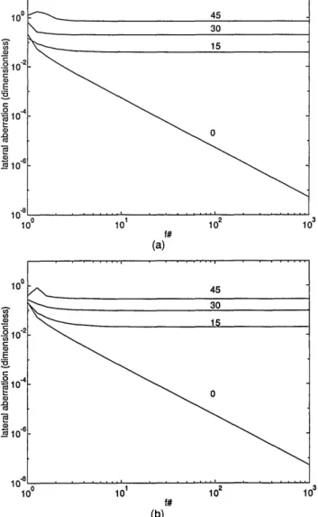
We begin by computing the geometrical spot sizes for the refractive and diffractive lenses described in Section 4. Figure 1 is calculated by ray tracing based
(a) (a)
(b)
Fig. 1. Geometrical spot size for a refractive lens with incidence angle 13 as a parameter: (a) tangential; (b) sagittal. The refrac-tive index has been taken as 1.5.
on Snell's law; Fig. 2 is calculated by ray tracing based on the first order of the grating equation. The spot size displayed in the figures is the root-mean-square (rms) lateral deviation (standard deviation) of the ray intercepts with the focal plane. The spot size is normalized with respect to D, the diameter of the lens, and thus is dimensionless. It is displayed as a function of f-number with incidence angle 13 as a parameter.
We conclude from the figures that the geometrical spot sizes for both types of lenses are similar within a factor of the order of unity. Since this is also true of the diffraction spot size to be discussed below, from now on we need not discuss both lenses separately. The normalized geometrical spot sizes in the tangen-tial and sagittal directions are denoted as &gl and &g2,
respectively.
The diffraction spot size in the tangential direction is given by6 Kf# Udl ldlX cos3 (2) 0 1 2 3 1 0 10 1 0 10 f# (b)
Fig. 2. Geometrical spot size for a diffractive lens with incidence angle p as a parameter: (a) tangential; (b) sagittal.
One of the cosine factors is related to the increased distance of propagation in the oblique direction, one to the reduced effective aperture, the other to the projection of the spot on the focal plane. Likewise, in the sagittal direction we have
Xf#
(d2-= d2X = Cos
(3)
Here the single cosine factor is related to the in-creased distance of propagation.
Then the total spot sizes (in meters) can be approxi-mated as
ul = &gl(f#,
)D
+ &dl(f#,P)x,
U2 = g2(f#, 13)D + &d2(f#,P)\-(4) (5) For a given wavelength K (which we take as 0.5 pum), the above expressions give a, and c2as functions of D,
f#, and P3.
In an information-processing or interconnection system for which it is desired to have a uniform and
isotropic resolution throughout the field, the syst spot size is given by the worst-case value
tem max{max[ia(0), A2()]>, (6) where the outer maximization is over . Since the spot size is an increasing function of
13,
it takes on its largest value at13
= 1ma. > 0, the field angle (Fig. 3). Thus the size of a resolution element of our system, u, is given by( = max[cri(Pm.), 2(13max)] (7)
Examining Figs. 1 and 2, and comparing identities (2) and (3), we can see that
ul
is always larger than a2SOthat a
= l(13ma).If we assume the wavelength to be
fixed, a is a function of the three variables D, f#, and Pmax.
Now, let us form our first figure of merit, the space-bandwidth product. This is defined as
N = (Xma)2
where Xma, is the linear field extent (Fig. 3). related to the field angle 1max by
2
=
f tan max =f#D tan
max.It is
As given, N is a function of D,
f#,
and 13max As max
is increased, the field extent Xmax also increases, but so does spot size a. For small max, the field is too small, whereas for large Pman, the aberrations become too large, so that there is an optimal value of 1
max
resulting in the largest N.
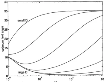
Maximizing over Pmac for each value of D andf#, we can eliminate the variable 13ma. The resulting depen-dence of N on D and f# is given in Fig. 4 as a contour plot. The optimal value of 13max as a function of f#
with D as a parameter is given in Fig. 5. Actually, N is very insensitive to the exact choice of Pmax; in most cases we can deviate 10°-20° from the optimal value
50 2c540 a a) 30 20 3 <4 2 0 5 10 15 1 log(f#) 20 25 30
Fig. 4. Contour plot of N as a function of D and f#. The contour levels give log N.
given in Fig. 5 and still obtain a value of N not much inferior to that given in Fig. 4.
Referring to Fig. 4, we observe that for small f#, increasing D has no effect on the space-bandwidth product. Likewise, for small D, increasingf# has no effect either. The space-bandwidth product can be increased by increasing both D and f# together. Accordingly the large value of N is observed in the upper-right region of the plot. As we move along belts of constant space-bandwidth product, we ob-serve a trade-off between D and f#; thus a suitable choice may be made depending on the relative diffi-culty of increasing these quantities in a particular implementation. Referring to Fig. 5, we observe that the optimum angle as a function of f# saturates to a particular value ( 35.2°) regardless of D, al-though the point of saturation depends on D. Roughly speaking, the optimal value of 13max increases
with f# (especially for smaller D) and assumes larger values for smaller values of D.
D 2 -D _ ', P ax f Xmax 2 - Xmax 2
Fig. 3. Definition of linear field extent Xni, and field angle PImax.
o 0o1 102 103
1 0 10 2
Fig. 5. Value of 03max maximizing N as a function f# with D as a parameter.
non. . . . . .. . .. au . ..
O _ _ _
Now, let us move on to our second figure of merit. The information density is defined as the space-bandwidth product divided by the cross-sectional area
of the system:
N
= max(X%., D2) (10)
The denominator is simply the minimum cross-sectional area of a tube in which our system can be enclosed. Geometrical factors of the order of unity are ignored. If bulk relaying of information is the only concern, the total capacity of the system can be increased by adding several parallel tubes. Note that when Xmax > D, I is simply given by l/U2. Once again, the expreession for I is a function of D, f#, and
13max-Maximizing over max, we obtain the information
density as a function of D and
f#
(Fig. 6). Notice that for a given value of D, there exists an optimum value off#
maximizing I, which we can read off the contour plot. On the other hand, for a given value off#,
decreasingD improves the information density up to a certain point, after which saturation occurs and further reduction of D does not result in any improve-ment. The largest value of I occurs at the lower-left corner of the graph, for small diameters and f-numbers.Figure 7 shows the optimal values of Clmax resulting
in maximum I. Once again, considerable latitude exists in the actual choice of Clmax- As
f#
increases,we see that the optimal value of maxc decreases, regardless of D. For the smaller values of D and f#, which we saw resulted in the largest information density, the optimal value of 13max is in the range
100-150.
Figure 8 displays the number of resolution cells Nlitho = (D/f#) 2 that the lithographic system pattern-ing the diffractive lenses must have in order to fabricate a lens with given diameter and f-number. In order that our formulation of Fresnel lenses be
Fig. 6. Contour plot of I as a function of D and f#. The contour
levels give log 1.
12 103
100 101 10 1
Fig. 7. Value of pm., maximizing I as a function f# with D as a parameter.
valid, D/f#k should not be too close to unity (say, > 10). Thus diffractive lenses corresponding to the lower-right region of f#-D space cannot be manufactured, a point that must be kept in mind when interpreting Figs. 4 and 6. (Strictly speaking, a Fresnel zone pattern with one or two rings can be manufactured, but it would not be of much use as a lens.)
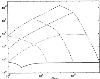
Figure 9 shows how N relates to Nlitho with f# and
D as parameters. The set of orthogonal grid lines
describes the region corresponding to the range of variation of D and
f#
used in our plots. The left-most region of this plot in which Nlitho is too close to 1 (say, Nlitho < 10) is, as mentioned, not admissible.For a given value of Nutho, we can find the largest possible value of N by drawing a line of constant Nlith. in Fig. 4. From this we would conclude that toward this end, it is desirable to increase both the diameter and the f-number as much as possible. Likewise, for
0)
0
0
5 1 0 1 5 20 25 30
1 olog(f#)
Fig. 8. Contour plot of Nitho as a function of D and
f#.
The contour levels give log Nitho. The region around and below the lowermost line is meaningless since here Njitho approaches or falls below unity.Fig. 10. Calculation of normalized by D.
G
T
iU~ei
f#
lateral aberration. All dimensions are
Fig. 9. N versus N1itho. The curves with positive inclination are curves of equal f-number (for the solid, dotted, dashed-dotted, and dashed curves, f# equals 1, 10, 100, and 1000, respectively). The curves with negative inclination are curves of equal diameter (for the same curve types, D/X equals 10, 103, 105, and 107, respec-tively).
a given value of N, the smallest possible value of Nlitho
can be found by drawing a curve of constant N in Fig. 8, from which we conclude that it is desirable to increase the f-number but to decrease the diameter. Both of these conclusions can also be read directly from Fig. 9 by drawing vertical or horizontal lines corresponding to constant Nllth. or N, respectively.
In a similar manner, one can draw a line of constant Nlith0 in Fig. 6 to determine what must be
done in order to increase I as much as possible for given Nlitho. In the upper-left region we observe that we should increase the diameter and the f-number, whereas in the lower-right region we observe that we should decrease both. Alternatively, a line of con-stant I superimposed in Fig. 8 tells us what to do in order to minimize N1itho for given I. In the upper-left
region we must decrease both the diameter and the f-number, whereas in the lower-right region we must decrease the diameter while keeping the f-number constant.
5. Analytical Discussion
Certain features of the results displayed in Figs. 4 and 6 can be explained analytically. Since the results for refractive and diffractive lenses are quite similar (see Figs. 1 and 2), we concentrate on diffractive lenses, which are simpler to analyze.
The deflection of rays from a diffraction grating (Fig. 10) is governed by the grating equation
sin o= sin
-=sinS-#X
(1
where Kf/x is the local periodicity of the Fresnel lens. Since we are interested only in the primary positive focal spot in which most of the energy is concen-trated, only the first order is considered. Here e = x/D and f# = f/D. The geometry of Fig. 10 leads to
= u(x = ED)
-)
D
f#(sin - t/f#)
[1 - (sin
13
- #/f#)2]1/
2 -f#
tan 13.This exact expression is the basis of Fig. 2(a). be expanded for small t/f# as
(e) (
2 os3"P1
Cos
PI)Jo (12) It can - 2( sin 13
)
B2f# cos3 B (13) - 3 1 CSince the range of
I I
is [0, 1/2], the requirement thatQlf#
be small is crudely satisfied for almost all values of f#. Then the variance of 6(e) can be calculated as=
f
[z(() - u]2d, (14) A2 2AB = )_4)-F _ + (3)(4) (4)(8) B2- 2AC (5)(16) + 2BC(6)(32)
C2 +(7)(64) (15) where the mean of az, which is close to zero, is ignored. When13
= 0, the above simplifies toA
8i_ 1fUrg =
8V7
16j_7(f#)2 (16)On the other hand, when
1
is sufficiently far from zero, 'g =Al
1 1 sin 2 2 1 1 -/ 2 2 cos 3 1cos (17)which we see is independent of f#. Equations (16) and (17) explain Fig. 2(a) for larger values of f#.
1 010 108 1 06 z 1 04 102 100 N litho 1 010 . . . I I . . ^ . . . . I. .," '' I, ... .... ... \ ... I'll ... \ . I 'I I ... .1.1 I .. .. I I ... .. 105 1 0o
Now let us use these analytical expressions to explain our numerical plots for the space-bandwidth product and information density. The expression for N becomes
N112 = 2f#D tan 1max
IA/hiD
+ f#X/cos3 .imaxX(18)
provided Oma is not too close to zero.Let us first examine the lower-right region of Fig. 4, in which f# is large enough that the second term in the denominator dominates. For this case we obtain
D
N1/2 (2
sin
woman COS213max) -* (19)Maximizing the respect to
max,we obtain sin
Pmax =xi/\;
thus 13max = 35.20 (the saturation value in Fig.5). Substituting this value of 3max in Eq. (19), we obtain
16 (D\2
N =
7 t A} * (20)This equation explains the dependence of N on D in the vertical direction on the right side of Fig. 4. For constant f#, N scales quadratically with D.
Now let us try to explain the upper-left region of Fig. 4. In this region the optimum value of Pmax does not exceed 100 or so (Fig. 5). For these relatively small angles we can simplify the trigonometric func-tions appearing in approximation (15) and show that the optimum value of Oman oc 1/f# and &g cC /(f#)2. (These results are consistent with Figs. 5 and 7.) In this region, geometrical effects are stronger than diffraction effects; thus
N = (Xmal/&gD)2 X (f#)4, (21) which explains the upper-left region of Fig. 4. We see that for larger diameters and smaller f-nuimbers, the space-bandwidth product increases with the fourth power of the f-number but is independent of the diameter.
Now, let us turn our attention to the information density. First, let us look at the lower-right region of Fig. 6. In this region it turns out that the largest value of I is attained when Xma,, = D. Recalling the expression for Xma. = 2f#D tan P3max, we see that this
implies that the optimal value of 13max is given by
1/2f# (consistent with Fig. 7). In this region, diffraction effects dominate so that
N1= 2 J12=max(Xm., D)
N'1/21
Xma =
which leads to I = (1/f#K)2, consistent with the lower-right region of Fig. 6. We observe that for larger f-numbers and smaller diameters the informa-tion density decreases with the square of the f-number but is independent of D.
Finally, turning our attention to the upper-left region of Fig. 6, in which it turns out that the optimum value of I is attained with Xma < D, we obtain
J1/2= N112 N'1 2 (f#)2
max(Xma., D) D c D
(23)
in which we used Eq. (21). This is consistent with the upper-left region of Fig. 6. For smaller f-numbers and larger diameters the information den-sity increases with the fourth power of the f-number and decreases with the square of the diameter.
In general, note that in the lower-right regions of our f#-D diagrams, in which the f# is much larger than D/X, diffraction effects dominate the spot size. On the other hand, in the upper-left regions of the same diagrams, geometrical effects dominate the spot size. The largest possible values of N and I occur when diffraction and geometrical effects are balanced, in the upper-right corner (for N) or in the lower-left corner (for I).
6. Conclusion
We have observed that to maximize the space-bandwidth product we need to work with large eters and large f-numbers. Obviously, large diam-eters increase the field size, improving the space-bandwidth product. Large f-numbers reduce the aberration spot, which also tends to increase the space-bandwidth product. Large f-numbers also in-crease the diffraction spot with respect to the size of a wavelength, but for large-diameter systems the aber-ration spot tends to dominate the diffraction spot so that the overall space-bandwidth product is in-creased by increasing the f-number as well.
Assume that we wish to send a certain amount of information through the smallest cross-sectional area possible or that we wish to send the largest possible amount of information through a given cross-sectional area. Should we use a single lens with diameter equal to the diameter of the informational channel or should we use many small diameter lenses in parallel? Since we saw that information density improves when we use systems with small lens diam-eters and small f-numbers, the latter will be more beneficial. Reducing the f-number reduces the dif-fraction spot as much as possible. Reducing the diameter reduces the aberration spot down to the size of the diffraction spot, resulting in the smallest possible overall spot size. The field size is small also, but this is compensated by the fact that the small diameter of the lens enables many such systems to be used in parallel. Thus the overall information den-sity is maximized with many small tubes rather than by a single lens.
We found that for diffraction-limited systems (large f-numbers and small diameters) the space-bandwidth product increases quadratically with the diameter and that the information density decreases quadrati-cally with the f-number. For geometrical
aberration-limited systems (large diameters and small f-num-bers) the space-bandwidth product increases with the fourth power of the f-number, and the information density increases with the fourth power of the f-number and decreases with the square of the diam-eter.
We have also derived relations between the space-bandwidth product, the information density, and the number of resolution cells that the lithographic sys-tem must have in order to produce the desired diffractive lens. The former are measures of perfor-mance, whereas the latter may be considered to be a measure of cost. From these relations it is possible to determine maximum performance for a given cost, or the minimum cost for given performance, as well as the choice of diameter and f-number necessary to attain these.
H. M. Ozakl as acknowledges support of the
Alex-ander von Humboldt Foundation during the initial phase of this research.
References
1. A. W. Lohmann, "Scaling laws for lens systems," Appl. Opt. 28, 4996-4998 (1989).
2. H. Nishihara and T. Suhara, "Micro Fresnel lenses," Prog. Opt. 24, 1-37 (1987).
3. J. T. Winthrop, "Propagation of structural information in optical wave fields," J. Opt. Soc. Am. 61, 15-30 (1971). 4. H. M. Ozaktas and D. Mendlovic, "Multistage optical
intercon-nection architectures with least possible growth of system size," Opt. Lett. 18, 296-298 (1993).
5. D. Mendlovic and H. M. Ozaktas, "Optical coordinate transfor-mation methods and optical interconnection architectures," Appl. Opt. 32, 5119-5124 (1993).
6. R. K. Kostuk, J. W. Goodman, and L. Hesselink, "Design considerations for holographic optical interconnects," Appl. Opt. 26, 3947-3953 (1987).