Perturbed orthogonal matching pursuit

Perturbed Orthogonal Matching Pursuit

Oguzhan Teke, Student Member, IEEE, Ali Cafer Gurbuz, Member, IEEE, and Orhan Arikan, Member, IEEE

Abstract—Compressive Sensing theory details how a sparsely

represented signal in a known basis can be reconstructed with an underdetermined linear measurement model. However, in re-ality there is a mismatch between the assumed and the actual bases due to factors such as discretization of the parameter space defining basis components, sampling jitter in A/D con-version, and model errors. Due to this mismatch, a signal may not be sparse in the assumed basis, which causes significant per-formance degradation in sparse reconstruction algorithms. To eliminate the mismatch problem, this paper presents a novel perturbed orthogonal matching pursuit (POMP) algorithm that performs controlled perturbation of selected support vectors to decrease the orthogonal residual at each iteration. Based on de-tailed mathematical analysis, conditions for successful reconstruc-tion are derived. Simulareconstruc-tions show that robust results with much smaller reconstruction errors in the case of perturbed bases can be obtained as compared to standard sparse reconstruction tech-niques.

Index Terms—Compressive sensing, basis perturbation, basis

mismatch, perturbed OMP.

I. INTRODUCTION

S

PARSE signal representations and the compressive sensing (CS) theory [1], [2] has received considerable attention in recent years in many research communities. In particular, CS changed the way data is acquired by significantly reducing the data acquisition number or cost, which has been applied to a wide range of important applications, such as computational photography [3], medical imaging [4], radar [5], [6] and sensor networks [7].

Compressive sensing states that a sparse signal in some known basis can be efficiently acquired using a small set of nonadaptive and linear measurements. Suppose dimensional signal has a -sparse representation in a transform domain

, as and . Given linear measurements in

the form , by using compressive sensing techniques, the sparse signal , hence , can be recovered exactly with very Manuscript received November 08, 2012; revised March 21, 2013, May 28, 2013, August 27, 2013; accepted September 10, 2013. Date of publication September 27, 2013; date of current version November 13, 2013. The associate editor coordinating the review of this manuscript and approving it for pub-lication was Dr. Ruixin Niu. This work was supported by TUBITAK within Career program grant Compressive remote sensing and imaging with project number 109E280 and within FP7 Marie Curie IRG grant Compressive Data Acquisition and Processing Techniques for Sensing Applications with project number PIRG04-GA-2008-239506.

O. Teke and O. Arikan are with the Department of Electrical and Electronics Engineering, Bilkent University, Ankara, 06800 Turkey.

A. C. Gurbuz is with the Department of Electrical and Electronics Engineering, TOBB University of Economics and Technology, Ankara, 06560 Turkey (e-mail: teke@ee.bilkent.edu.tr; oarikan@ee.bilkent.edu.tr; acgurbuz@etu.edu.tr).

Color versions of one or more of the figures in this paper are available online at http://ieeexplore.ieee.org.

Digital Object Identifier 10.1109/TSP.2013.2283840

high probability from measurements by solving a convex optimization problem of the following form:

(1) which can be solved efficiently using linear programming. Stable reconstruction methods for noisy measurements or compressible signals based on minimization have been de-veloped [8]–[10] for the known basis case. Suboptimal greedy algorithms have also been used in many applications. Matching pursuit (MP) [11], orthogonal matching pursuit (OMP) [12], compressive sampling matching pursuit (CoSaMP) [13], iter-ative hard/soft thresholding (IHT) [14] are among the most commonly used greedy algorithms. Apart from greedy algo-rithms, approximate message passing (AMP) uses the idea of belief propagation to achieve high reconstruction performance with low complexity [15]. If the sparse signal has a structure, such as a wavelet tree, techniques proposed in [16] can exploit those models for better reconstruction. The study in [17] as-sumes a Markov-tree structure in the sparse coefficients and adapts the AMP algorithm in a Bayesian framework.

Commonly used sparse reconstruction techniques assume that the basis is exactly known and the signal is sparse in that basis. However, in some applications there is a mismatch between the assumed basis and the actual but unknown one. For example in applications like target localization [18], radar [19], [20], time delay and doppler estimation, beamforming [21], [22] or shape detection [23], the sparsity of the signal is in a continuous parameter space and the sparsity basis is constructed through discritization or gridding of these param-eter spaces. In general, a signal will not be sparse in such a dictionary created through discritization, since no matter how fine the grid dimensions are, the signal parameters may not, and generally do not, lie in the center of the grid cells. As a simple example; consider a general signal which is sparse in the continuous frequency domain. This signal may not be sparse in the DFT basis defined by the frequency grid. A continuous frequency parameter lying between two successive DFT grid cells will affect not the only the closest two cells, but the whole grid with amplitude decaying with , where T is the sampling time interval. This off-grid phenomena violates the sparsity assumption, resulting in a decrease in reconstruction performance. In addition to these structured perturbations, random time jitter in A/D conversion, modeling errors in construction of the dictionary create perturbations on the dictionary columns. Hence, in general, the signal will

be sparse in an unknown basis where is the

adopted basis and is the unknown perturbation matrix. In the literature, the effect of this basis mismatch has been observed and analyzed in some applications such as radar [19], [24] and beamforming [25]. In problems due to parameter space discritization, a simplistic approach is to use multi-resolution re-finement and decrease the grid size. Decreasing the grid size is 1053-587X © 2013 IEEE

not a direct solution to the basis mismatch problem, because it increases the coherence between dictionary columns, violating the restricted isometry property (RIP) [26] and increasing the computational complexity of the reconstruction. In [27]–[29] the effect of the basis mismatch problem on the reconstruction performance of CS has been analyzed and the resultant perfor-mance degradation levels and analytical norm error bounds due to the basis mismatch have been investigated. However, these works do not offer a systematic approach for sparse recon-struction under random perturbation models. In [30], the dictio-nary is extended to several dictionaries and solution is pursued not in a single orthogonal basis, but in a set of bases using a tree structure, assuming that the given signal is sparse in at least one of the basis. However, this strategy does not provide solutions if the signal is not-sparse in the extended dictionary. In the Con-tinuous Basis Pursuit approach [31], perturbations are assumed to be continuously shifted features of the functions on which the sparse solution is searched for, and based minimization is proposed. Also in this method, perturbations are assumed to have structure, and are modeled with a first order Taylor approx-imation or polar interpolators. In [32], minimization based algorithms are proposed for linear structured perturbations on the sensing matrix. In [33] a total least square (TLS) solution is proposed for the problem, in which an optimization over all signals , perturbation matrix and error vector spaces should be solved. To reduce complexity, suboptimal optimization tech-niques have been pursued in [33].

In this paper, a novel perturbed orthogonal matching pursuit (POMP) algorithm is presented. In the standard OMP algorithm [12] the column vector that has the largest correlation with the current residual is selected and the new residual is calculated by projecting the measurements onto the subspace defined by the span of all selected columns. This procedure is repeated until the termination criteria is met. In the proposed POMP al-gorithm, controlled perturbation mechanism is applied on the selected columns. The selected column vectors are perturbed in directions that decrease the orthogonal residual at each itera-tion. Proven limits on perturbations are obtained. The proposed method is fast, simple to implement and successful in recovering sparse signals under random basis perturbations. A preliminary form of this approach has been presented in [34].

The organization of the paper is as follows. Section II out-lines the formulation of the problem and details the development of the proposed POMP algorithm with a pseudo code and sup-porting theorems. Results covering performance comparisons of the proposed method and applications on a set of examples are given in Section III. In Section IV, concluding remarks are pre-sented and detailed proof of a theorem is given in the Appendix.

II. PERTURBEDORTHOGONALMATCHINGPURSUIT In compressive sensing, a sparse signal is reconstructed from its given underdetermined linear measurements:

(2)

where with and is

addi-tive noise, typically assumed to be independent and identically distributed (i.i.d.) Gaussian noise with known variance . The

matrix may be known, as in the case of row decimated ver-sions of Fourier or wavelet transformation matrices, or it might be a randomly selected one. The ideal reconstruction problem can be formulated as an minimization problem,

(3) where is the cardinality of , and the fit error constraint has a bound that is related to the measurement noise statistics. However, solution of the minimization problem requires a combinatorial search, thus it is not feasible for practical applications.

Another challenge is reconstruction in the presence of errors in . When is not known precisely, may not be sparse in the assumed . However, sparsity of the signal can be revealed under a certain perturbation, , on the given . In this case, the problem can be recast as,

(4) where is some bounded perturbation space. This problem can be viewed as a generalized version of the problem given in [31], in which is considered as a Taylor series or polar approxi-mation of and is the sufficient limits, also relaxing with . The solution to this general problem is also combinatoric in nature, and infeasible in practice.

To reduce the complexity of the problem of (4), sub-op-timal greedy techniques can be developed as well. In these greedy approaches, the support set of the reconstruction is iter-atively increased until the constraints are satisfied. Assuming that at iteration , the support set contains columns of ,

which we will call as for simplicity. At

the th iteration, new vector is obtained from the solution of the following optimization problem:

(5) where matrix is the projection operator to the column space

of perturbed and is the set of all

basis vectors that are not contained in . For each , this perturbation problem can be solved by using the technique given in [35]. However, due to its associated gradient descent based iterations, the complexity of solution is still a practical limitation for large . In this work, we propose a simpler non-iterative perturbation for each , to maximize the projection under bounded perturbations. At any iteration , the measurement can be decomposed as:

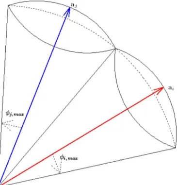
(6) where is the projection of onto the span of vectors in and is the orthogonal residual. Since vectors in are lin-early independent, this projection can be uniquely expressed as: (7) where is the weight of the corresponding th column vector. In the proposed approach, as shown in Fig. 1, the ’s will be

Fig. 1. One dimensional example for perturbed and unperturbed column vec-tors. As the basis vector rotates, residual decreases.

perturbed by rotating them towards to by an angle , where is the normalized residual:

(8) Since both and have unit norms and they are orthog-onal to each other, , which is the perturbed version of , has also unit norm. If the angle of rotation, or equivalently, the al-lowed amount of perturbation on is large enough, then can be aligned with and there will be no residual left in the perturbed basis. If the ’s are rotated more than adequate, ’s can overlap with each other. When more than one vector span the overlapping region, uniqueness of the projection is lost. In order to avoid such overlaps, rotation of should be limited to the half of the minimum angle between and other for . More precisely, the maximum perturbation angle, , for a vector should satisfy:

(9)

where is the mutual coherence of and

. This case is illustrated in Fig. 2, where the maximum allowed perturbation of a vector is such that the cones around the columns of do not overlap with each other. Perturbations beyond this limit generate switch-over between the chosen set of vectors and cause non-unique projection. Therefore, at each step of the proposed approach, only pertur-bations satisfying this limit will be considered.

The approach of perturbations embedded in the iterations of Orthogonal Matching Pursuit(OMP) provides a practical tech-nique for sparse reconstruction when basis mismatch is present. In the following discussion, we will provide a detailed theoret-ical investigation of this approach that will be referred to as Per-turbed-OMP, or POMP in short.

Theorem 1: For the largest perturbation angle satisfying

and , the perturbed

sup-port vectors defined in (8), has an orthogonal residual whose norm is upper bounded as:

Proof: From (8), can be written as:

(10)

Fig. 2. Each unit column of has a maximum perturbation angle so that the perturbed vectors do not overlap with each other.

Replacing this decomposition of in terms of and in (7), measurements can be written as:

(11) which can be regrouped to obtain:

(12) In this decomposition of , the second term is in the span of the perturbed vectors . Therefore, the orthogonal decompo-sition of in the perturbed basis is:

(13) where is the projection of onto the span of the perturbed basis vectors, and is the corresponding residual. Thus,

(14) Since, the norm of the projection operation is less than one, we have:

From the hypothesis, , thus we obtain the desired upper bound:

(16)

The proof of Theorem 1 also reveals the following fact: Corollary 1: The upper bound derived in Theorem 1 is mono-tonically decreasing as a function of as long as the condition

is satisfied. Proof: In Theorem 1, it is shown that:

As long as , the right hand side is a

valid non-negative upper bound for , and is a continuous

function of all , with partial derivatives:

(17) which are all strictly negative for . Thus, the upper bound decreases monotonically as a function of , q.e.d.

The first implication of Corollary 1 is that once a candidate

support set is available and , rather

than searching for a perturbation that minimizes , one can minimize its upper bound simply by perturbing each vector in the support up to its allowed limit.

The second implication of Corollary 1 is that if the perturba-tion angles are increased, i.e., more freedom for the adjustment of the basis exists, the derived upper bound decreases. There-fore, for a certain amount of perturbation, this raises the possi-bility of driving the upper bound to zero.

Corollary 2: Let . Then if

, perturbation of the support vectors up to , results in , yielding a -sparse reconstruction with no residual error.

Proof: Simply replace

in the upper bound given in the (16) to get:

(18)

It is important to note that Theorem 1 and Corollaries 1 and 2 are valid for any set of linearly independent vectors from the columns of . Even though chosen subset does not include any component from the correct support, this theorem guaran-tees that by using perturbation, the residual can be decreased. If is the correct support, or some subset of the correct support,

then becomes a good approximation of . In this

case, becomes smaller and hence , the angle of per-turbation at which the upper bound becomes zero, is a smaller angle.

Proposition 1: A perturbed set of support vectors

will have if and only

if the upper bound in (16) is zero.

Proof: Using perturbations up to , the residual will be zero; hence we can expand as:

(19) Assume there is another angle resulting also a zero residual. Hence, we can expand as:

(20) If we subtract (19) from (20) term by term, we get the fol-lowing:

(21) Since and are orthogonal to each other,

and . If we divide both

equa-tions term by term, we get . Since we only

consider acute angles, , which contradicts the assump-tion. Hence, the perturbation angle which results upper bound in (16) to be zero is unique, q.e.d.

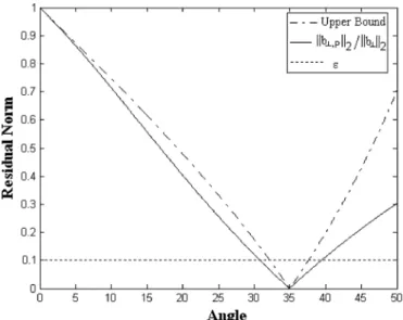
Although in the proposed perturbation approach norm of the residual can be made zero for large enough perturbation angles, a relaxed constrained optimization problem, where

, is more appropriate when there is noise in . Under this re-laxation, more sparse reconstructions can also be obtained. In Fig. 3 as an illustrative case, the error residual is shown as a function of perturbation angle. It is seen that the constraint line intersects with the error norm curve at , which is the first intersecting angle smaller than . The following the-orem provides an estimate for by using the intersection of

with the upper bound in (16).

Theorem 2: If the perturbation angles of support vectors in

are all chosen as , where

Fig. 3. Upper bound and as a function of .

Proof: If in (16) is replaced with , then the upper bound becomes:

(22) Note that for small enough , the residual error of projec-tion onto the perturbed support vectors, i.e., , the above bound will also be tight and will be close to . Therefore, for the th iteration of the proposed POMP approach, there are three limits on the perturbation angles: first, , which is the limit predefined by the coherence of as defined in (9); second , beyond which the residual error norm is lower than ; and third , the user-defined limit. A user may want a solution with larger or smaller perturbations and, therefore may want . Hence, the allowable perturbation angle for the th support vector should be

(23) In general, is a larger angle compared to other two. In the early phases of POMP, where the number of chosen support vectors are lower than actual sparsity level, is expected to be larger than the allowed perturbation, . Therefore, in the early phases of the iterations, the residual error norm of the perturbed support vectors is typically larger than the termination criterion . Yet, it is expected that as new columns are added to the cur-rent support during the iterations, will decrease and will be

less than eventually. Once ,

iterations will stop, since after the perturbation the residual will have a norm less than . The following theorem, whose proof is provided in the Appendix, states this expectation formally.

Theorem 3: Let be the support estimation in the th it-eration and be the required perturbation angle as derived in Corollary 2 and let be the basis vector chosen in the

TABLE I

PERTURBED-OMP (POMP) ALGORITHM

th iteration. If , then, ,

where .

Since is full rank, iterations stop when reaches without any perturbation in the worst case. Therefore, is zero. According to Theorem 3, when the required condition is satisfied, produces a monotonically decreasing sequence throughout the iterations. Since we know that , there

exists a such that due to monotonicity of the

angles. Therefore, Theorem 3 indirectly guarantees the termi-nation of iterations.

It is important to note that Tropp’s Exact Recovery Condi-tion for OMP [36], which simply states that if for all un-selected basis vectors, OMP will select one of the cor-rect support vectors in the next iteration, is a stricter version of Theorem 3. Hence, we can safely guarantee that maximum required angle, , will always decrease throughout the itera-tions as long as OMP is guaranteed to provide exact reconstruc-tion. This point will be revisited with numerical simulations in Section III.

The steps of the proposed Perturbed Orthogonal Matching Pursuit (POMP) algorithm is detailed in Table I. Starting with a set of unit norm vectors, in the th iteration, POMP searches over the dictionary to find the vector providing the largest ab-solute inner product with the residual. After the selection of the new vector, POMP computes the projection of the measurement, , onto the new larger support and finds the residual. OMP con-tinues with the next iteration here. However, POMP proceeds with the perturbation. Given and is computed according to (23). It is assumed that user provides an angle, , less than

the mutual coherence of the basis, ,

oth-erwise perturbations are limited by the basis itself. After that POMP starts to perturb each vector in the current support as given in (8). Then, the measurement vector, , is projected onto the perturbed support and the new residual is found. If the norm

of the residual is less than , iterations are terminated, otherwise POMP continues with the next iteration.

One important characteristic of POMP is the promise of the sparser solutions. This property can be revealed as follows. As-sume that POMP has produced a -sparse solution. Iterations can be terminated due to two reasons. If the observation is al-ready sparse in , then at the th iteration we get . Since OMP and POMP have the same selection criteria, OMP also chooses the very same and obtains the same sparse solution. However, if is not sparse in , POMP obtains the

sparse solution using the perturbation. Since

but , OMP iterates at least one more time resulting a denser solution. Therefore, for any observation , OMP pro-duces denser, or equally sparse at best, solutions than POMP.

OMP is preferred in many applications due to its computa-tional efficiency. In the perturbation stage of the proposed algo-rithm, the inverse tangent operation can be well approximated by using tables and low order power series expansion, therefore the computational order is determined by the least-squares solu-tion on the perturbed basis, which has a complexity of

in the th iteration, which is the same as the standard OMP algo-rithm. If the algorithm terminates in the th iteration, overall

complexity becomes for both POMP and OMP. In

the worst case, algorithm will terminate eventually in the th iteration, which results in complexity of .

III. SIMULATIONRESULTS

In this section, performance of POMP algorithm will be investigated and compared with alternative techniques under random basis mismatch. For this purpose, sparse reconstruction of sinusoids from their time samples will be considered. In this example, following dictionary vectors are used:

(24) where is the frequency of the th dictionary vector and is the vector of time samples at which the signal is sampled. However, in practice, due to time jitter in the sampling, the observed signal is not sampled at the nominal sampling times, resulting in a dictionary mismatch:

(25) where can be modeled as a vector of independent and uniformly distributed random variables in the range of where represents the level of jitter. The overall effect of time-jitter can be considered as a random

perturbation on the dictionary . In this more

realistic scenario, is typically non-sparse in the assumed dictionary .

In the first simulation, the dictionary is constructed by using

frequencies Hz for and frequency

separation of Hz. The sampling time vector is created over the second interval with randomly chosen

time samples. A 25-sparse signal is randomly generated with non-zero coefficients selected uniformly random from the range . Observations, , are generated with time jitter of sec. The same termination criteria of

is used for all compared techniques.

To select a proper maximum perturbation angle for POMP, the expected value of the perturbation angles are calculated. Based on the following, the normalized inner products of

and :

Since the sampling jitter is modeled as an i.i.d.

se-quence, and

for large . Therefore, the expected value of the cosine of the perturbation angles can be approximated as:

(26) Using the small angle approximation of cosines, (26) can be further simplified as:

where is the jitter variance. Since jitter is assumed to be

uniform in the interval . Finally,

using a small angle approximation for , we obtain,

(27) Therefore, in the implementation of POMP, the allowed pertur-bation angles are selected according to (27) for each column, respectively. For the th column of that corresponds to

Hz, the maximum perturbation angle is .

Fig. 4 shows actual and reconstructed signal coefficients for OMP and POMP techniques for a random realization of jitter. In this specific case, while POMP correctly reconstructs the sparse signal coefficients, OMP generates a highly non-sparse signal. For this realization, Fig. 5 shows , the Tropp’s Exact Recovery Condition (ERC) [36] and the proposed bound of The-orem 3. Even though ERC is not satisfied for , the pro-posed conditions of Theorem 3 are satisfied for this case. There-fore, this example shows that, the guarantees given by Theorem 3 provide a larger regime in which POMP is successful.

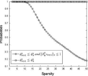
In this section of the simulations, we will investigate perfor-mance of POMP when the condition of the Theorem 3 is not sat-isfied. For this purpose, we conduct a large set of Monte-Carlo simulations in excess of trials in which the sparsity level and number of measurement are swept from 2 to 85 and to 200, respectively. For each pair, 100 cases are simulated. In each of these simulations, cases where the pertur-bation angle decrease, i.e., , are identified as event , and the sufficiency condition of Theorem 3 is satisfied, i.e., , are identified as . Out of all the runs at each sparsity level, the cases where only is valid and both

Fig. 4. A realization of the reconstruction problem under time-jitter where OMP drastically fails and produces 167-sparse solution.

Fig. 5. and its bound as a function of iterations. Even though ERC is not satisfied for , condition in Theorem 3 is satisfied due to large value of , ensuring the decrease of maximum perturbation angle during the iterations.

and are valid are counted separately. In Fig. 6, the statis-tics of the cases are shown for all the experiments conducted.

It can be observed that for , the case is satisfied with empirical probability of 1, and as sparsity level increases, the probability of the case being satisfied decreases. The max-imum perturbation angle decreases consistently when the case is satisfied. Note that, Theorem 3 is only a sufficiency condi-tion and in the simulated scenario for its requirements are not guaranteed to met. Nevertheless, in all the simulations conducted, it is observed that the perturbation angle decreases. To compare the overall performance in the above described set of simulations, the following metrics are used: the

nor-malized signal reconstruction error, ; the

level of sparsity, ; the distance between signal

sup-ports, ; and the normalized residual norm,

, where is the correct signal and its support, and is the obtained solution and its corre-sponding support [37].

Fig. 6. Empirical probabilities of is valid and is jointly valid.

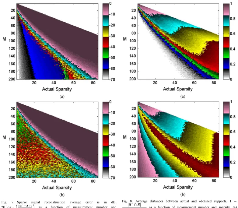
In Figs. 7 and 8, the average performance results obtained for OMP and POMP are shown. Fig. 7 shows the normalized re-construction error for both OMP and POMP in dB, while the corresponding support distances can be seen in Fig. 8. For the same number of measurements and range of sparsity levels, it can be observed from Fig. 7 that both OMP and POMP have similar phase transition curves; however POMP produces sig-nificantly lower reconstruction errors. In Fig. 8, it can be seen that POMP provides more reliable supports as well.

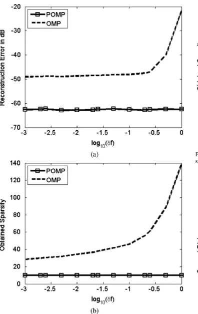
Instead of using perturbation procedure, one can try to use OMP in a finely discretized frequency domain. This way, the required perturbations on the dictionary vectors can be reduced. However, increasing the density of the basis also increases the coherence of the dictionary which adversely affects per-formance of the CS techniques. In the simulated scenario, the effect of increasing frequency density in the dictionary is shown in Fig. 9. In this case number of measurements is kept constant at , however the size of the dictionary is increased

as . The frequency range of Hz

is considered in the simulations. Random time samples are

chosen in time interval with a jitter of sec

time jitter. Compared to , when is

used, this corresponds to approximately 1000 times denser sampled frequency dictionary with . Sparsity of the signal is kept constant at , and the SNR of the observed signal is kept at 60 dB to better observe the effect of using a denser dictionary in the reconstructions. As seen in the Fig. 9(a), using a denser basis can decrease the reconstruction error up to approximately dB for OMP. However, beyond this point, OMP reaches an error floor. Also, as seen from Fig. 9(b), obtained sparsity is reduced significantly. On the other hand, reconstruction performance of POMP is almost independent from the density of the dictionary. For all tested cases of , POMP has a reconstruction error below dB and yields a 10 sparse solution, that matches the actual sparsity. Note that using a denser basis significantly increases the mutual correlation of the dictionary vectors as well as the required number of inner-products. Therefore, rather than using OMP

Fig. 7. Sparse signal reconstruction average error is in dB, as a function of measurement number and sparsity. (a) POMP. (b) OMP.

over a larger and denser dictionary, it is advisable to use POMP over a moderate size dictionary. Note that if the frequencies of the signal components were known precisely, the linearization based techniques proposed in [32], [33], [38] could have been used for the estimation of the jitter in the sampling times.

In this part of the simulations, we compare POMP with OMP, CoSaMP, Basis Pursuit, and Sparse Total Least Squares (S-TLS) [33] algorithms. Since POMP is based on OMP iterations, they have similar phase transition characteristics as given in Fig. 7. Hence, in the following simulations, we will stay in the regime in which OMP works successfully.

Unlike OMP and POMP, CoSaMP requires the correct spar-sity level of the signal. Since, such information is not avail-able in general, CoSaMP reconstructions obtained at all sparsity levels starting from until the residual error is below the specified level.

Basis Pursuit (BP) which is also known as reconstruction is implemented using the convex optimization toolbox CVX. To

Fig. 8. Average distances between actual and obtained supports, as a function of measurement number and sparsity. (a) POMP. (b) OMP.

induce sparsity, hard thresholding is applied to BP reconstruc-tion results. Let be the BP reconstruction sorted in the absolute sense and be the vector containing largest coefficients. Then, in the reported results here, the threshold, ,

is selected as such that .

In [33], two algorithms have been proposed for S-TLS; one finds the global optimum with highly demanding computational cost, and the other one is computationally more efficient but only guaranteed to converge to a local minima. Here, this more efficient technique which is called as coordinate descend (CD) based S-TLS is used for comparison. Since S-TLS has an it-erative structure, the stopping criteria is important. To obtain a consistent comparison of algorithms, S-TLS is terminated when the residual error is below the specified at the end of an iter-ation. Rather than an all-zero vector, iterations are started with the solution of the obtained BP reconstruction to achieve faster convergence for S-TLS. In the following results, STLS-1

Fig. 9. Reconstruction performance with respect to density of the complex ex-ponentials. (a) Sparse signal reconstruction error in dB, (b) Obtained sparsity level for POMP and OMP algorithms.

where is the sparsity-tuning parameter of the CD based S-TLS algorithm.

For all the techniques compared, Figs. 10 and 11 shows the obtained sparsity levels and support distances as a function of sparsity, respectively. POMP and S-TLS, being perturbation based techniques, can achieve the correct sparsity level for smaller . As the actual sparsity increases, S-TLS fails to ob-tain the correct sparsity, whereas POMP successfully finds the support up to . Techniques that do not employ dictio-nary perturbation provided results that are significantly inferior than POMP and S-TLS at all sparsity levels. The performance of these techniques saturates and produce solutions at about the same sparsity, irrespective of the actual sparsity level. Since the observed signal is not sparse in the assumed dictionary with , OMP goes up to two-third of the rank whereas CoSaMP uses approximately 90% of the rank. On the other hand, POMP obtains the correct sparsity level and the support as shown in Fig. 11. S-TLS gradually produces higher support distances due to denser solutions obtained in less sparse

Fig. 10. Obtained sparsity of the reconstructed signal as a function of actual sparsity.

Fig. 11. Distances between actual and obtained supports as a function of actual sparsity.

signals. Since techniques that do not employ perturbation has

a saturated sparsity estimate, , and

increases gradually as increases. Therefore, their distance metric produces smaller values. However, this situa-tion should not be considered as performance improvement for less sparse signals. It is because they simply fail to recover the correct support at all tested sparsity levels.

Fig. 12 shows the average normalized reconstruction error in dB as a function of true sparsity for each of the compared re-construction techniques. As expected, BP performs better than OMP. However, even though S-TLS employs perturbation, it has very similar performance to BP. POMP, on the other hand, has a significantly lower, dB, signal reconstruction error as compared to S-TLS and BP. CoSaMP has the worst perfor-mance among all the compared techniques with significantly higher reconstruction errors.

In the above simulations, termination criteria of all algorithms are determined by the residual norm level . We assume that

Fig. 12. Signal reconstruction error in dB as a function of actual sparsity.

observation has the form of . If we write

the residual as,

(28)

hence if noise variance is small.

Therefore, can be chosen. More specifically, if the

noise has a variance , then . Since the

sig-nals are error free in previous simulations, is chosen. However, if the signal comes from a perturbed dictionary, then

, hence,

(29) where noise and perturbations are assumed to be independent. It is appropriate to define

(30) as the Signal-to-Perturbation Ratio (SPR). Therefore according

to (29), . In our

frame-work, , since .

Using simple geometry, the perturbation amount can

be written as . Hence, the

perturbation amount is ,

where . Therefore,

. If the perturbations are small, it can be approximated as:

(31) In the following simulations, we aim to analyze the SNR and SPR regions in which POMP and compared techniques can suc-cessfully work. For this purpose sparsity is fixed at and average reconstruction performance is found for varying SNR and SPR levels.

In Fig. 13, the perturbation level is kept constant at

dB, which corresponds to sec according to (31), and the SNR is varied from 20 dB to 60 dB. In Fig. 14, we keep

the noise level constant at dB and the is

varied from 30 dB to 70 dB. In both figures, the reconstruction

Fig. 13. Signal reconstruction error in dB for fixed dB and varying SNR from 20 dB to 60 dB.

Fig. 14. Signal reconstruction error in dB for fixed dB and varying SPR from 30 dB to 70 dB.

performances are shown as a function of the

Noise-to-Perturba-tion Ratio (NPR) defined as . It

is clear that two distinct performance regions are determined by

the sign of .

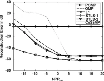
As shown in Fig. 13, although POMP has the lowest re-construction error, all compared techniques have acceptable performances for positive . In that regime, noise power dominates the perturbation on the dictionary. Since the perturba-tions are relatively insignificant, OMP and CoSaMP can achieve similar results to POMP. However, when is negative, the perturbation on the dictionary is more dominant than the noise level. OMP, BP and CoSaMP have no mechanism to handle these perturbations, hence they treat the perturbations as additional noise. However, in this case it is highly improbable to decrease the residual error to the actual noise level. Thus, they saturate and produce reconstructions with larger errors. On the other hand, even if perturbations dominate the noise, POMP can handle perturbations and produces reconstruction with significantly lower errors. Fig. 14 displays similar results, where SNR is fixed

and SPR is varied. For high NPR regime, all algorithms result in similar errors, whereas for low NPR, only POMP produces acceptable reconstructions. Higher perturbation causes larger reconstruction errors in POMP. However, it is much more robust to dictionary mismatch than the compared techniques.

IV. CONCLUSION

Compressive sensing reconstruction techniques suffer from significant performance degradation when there is a mismatch between the actual and the chosen signal dictionaries. Such mis-match generally occurs in practice due to modeling errors, pa-rameter space discritization or simply by sampling jitter. In gen-eral, this mismatch problem cannot be solved using denser basis. Also, density of the basis adversely affects the algorithms due to high correlation. In this paper, a novel perturbed greedy recon-struction technique is proposed for the case of signal reconstruc-tion in the presence of perturbareconstruc-tions in the signal dicreconstruc-tionary. The proposed Perturbed OMP (POMP) technique performs con-trolled perturbations of selected support vectors. Limits on the required perturbation for exact fit to observation signal at any sparsity is found. Also, for a given acceptable residual level, limits on the required perturbation are also provided. A suf-ficiency condition that assures monotonic decrease on the re-quired perturbations as a function of sparsity is given. The per-formance of the proposed algorithm is investigated on a time jitter example that causes a random dictionary mismatch. As an extension to SNR, Signal-to-Perturbation (SPR) and Noise-to-Perturbation (NPR) are used for better characterization of the performance limits of POMP. Results show that, in comparison with well known CS reconstruction techniques, POMP provides efficient reconstructions with significantly lower reconstruction error in a wide range of sparsity levels.

APPENDIX PROOF OFTHEOREM3

Let be the matrix whose columns

cor-respond to the current estimate for the support of . Since is

full rank, we can define and .

The following equations provide recursive relations for

and :

(32) (33)

where and . Since

the norm of a partitioned vector is the sum of the norms of each partition:

(34)

which can be written as:

(35)

where and .

To have , we need the following inequality to hold true:

(36) Using the triangle inequality on (35), the following bound can be obtained,

(37)

Since , (37)

be-comes:

(38)

By adding to both sides of (38), we obtain:

(39) The desired condition on angle decrease requires

, which is always achieved if:

(40) or equivalently:

(41) Therefore, by using (36), (41) and definition of , the non-negative constant in the statement of Theorem 3 can be ob-tained as:

(42)

REFERENCES

[1] D. Donoho, “Compressed sensing,” IEEE Trans. Inf. Theory, vol. 52, no. 4, pp. 1289–1306, 2006.

[2] E. Candes, J. Romberg, and T. Tao, “Robust uncertainty principles: Exact signal reconstruction from highly incomplete frequency infor-mation,” IEEE Trans. Inf. Theory, vol. 52, pp. 489–509, 2006. [3] M. D. ad, M. Davenport, D. Takhar, J. Laska, T. Sun, K. Kelly, and

R. Baraniuk, “Single-pixel imaging via compressive sampling,” IEEE

Signal Process. Mag., vol. 25, no. 2, pp. 83–91, 2008.

[4] M. Lustig, D. Donoho, and J. Pauly, “Sparse MRI: The application of compressed sensing for rapid MR imaging,” Magn. Reson. Med., vol. 58, no. 6, pp. 1182–1195, Dec. 2007.

[5] R. Baraniuk and P. Steeghs, “Compressive radar imaging,” in Proc.

IEEE Radar Conf., 2007, pp. 128–133.

[6] V. Patel, G. Easley, D. H. Jr., and R. Chellappa, “Compressed synthetic aperture radar,” IEEE J. Sel. Topics Signal Process., vol. 4, no. 2, pp. 244–254, 2010.

[7] W. Bajwa, J. Haupt, A. Sayeed, and R. Nowak, “Compressive wire-less sensing,” in Proc. Int. Conf. Inf. Process. Sens. Netw. (IPSN), Apr. 2006, pp. 134–142.

[8] E. Candès, J. Romberg, and T. Tao, “Stable signal recovery from in-complete and inaccurate measurements,” Commun. Pure Appl. Math., vol. 59, no. 8, pp. 1207–1223, 2006.

[9] J. Haupt and R. Nowak, “Signal reconstruction from noisy random pro-jections,” IEEE Trans. Inf. Theory, vol. 52, no. 9, pp. 4036–4048, 2006. [10] D. Donoho, M. Elad, and V. Temlyakov, “Stable recovery of sparse overcomplete representations in the presence of noise,” IEEE Trans.

Inf. Theory, vol. 52, no. 1, pp. 6–18, 2006.

[11] S. Mallat and Z. Zhang, “Matching pursuits with time-frequency dic-tionaries,” IEEE Trans. Signal Process., vol. 41, 1993.

[12] J. Tropp and A. Gilbert, “Signal recovery from random measurements via orthogonal matching pursuit,” IEEE Trans. Inf. Theory, vol. 53, no. 12, pp. 4655–4666, Dec. 2007.

[13] D. Needell and J. Tropp, “Cosamp: Iterative signal recovery from in-complete and inaccurate samples,” Appl. Computat. Harmon. Anal., vol. 26, no. 3, pp. 301–321, 2009.

[14] T. Blumensath, M. Yaghoobi, and M. Davies, “Iterative hard thresh-olding and regularisation,” in Proc. ICASSP, 2007, vol. 3, pp. 877–880.

[15] D. L. Donoho, A. Maleki, and A. Montanari, “Message passing algo-rithms for compressed sensing,” Proc. Nat. Acad. Sci., vol. 106, no. 45, pp. 18 914–18 919, Nov. 2009.

[16] R. G. Baraniuk, V. Cevher, M. F. Duarte, and C. Hedge, “Model-based compressive sensing,” IEEE Trans. Inf. Theory, vol. 56, no. 4, pp. 1982–2001, Apr. 2010.

[17] S. Som and P. Schniter, “Compressive imaging using approximate message passing and a Markov-tree prior,” IEEE Trans. Signal

Process., vol. 60, no. 7, pp. 3439–3448, Jul. 2010.

[18] V. Cevher, M. Duarte, and R. Baraniuk, “Distributed target localization via spatial sparsity,” in Proc. Eur. Signal Process. Conf. (EUSIPCO), Aug. 2008, pp. 134–142.

[19] J. H. Ender, “On compressive sensing applied to radar,” Signal

Process., vol. 90, no. 5, pp. 1402–1414, 2010.

[20] A. C. Gurbuz, J. H. McClellan, and W. R. Scott Jr., “A compressive sensing data acquisition and imaging method for stepped frequency GPRS,” IEEE Trans. Signal Process., vol. 57, no. 7, pp. 2640–2650, 2009.

[21] A. C. Gurbuz, V. Cevher, and J. H. McClellan, “A compressive beam-former,” in Proc. ICASSP 2008, Las Vegas, NV, Mar. 30–Apr. 4 2008. [22] Y. Yu, A. P. Petropulu, and H. V. Poor, “MIMO radar using compres-sive sampling,” IEEE J. Sel. Topics Signal Process., vol. 4, no. 1, pp. 146–163, 2010.

[23] N. Aggarwal and W. C. Karl, “Line detection in images through reg-ularized Hough transform,” IEEE Trans. Image Process., vol. 15, pp. 582–590, 2006.

[24] M. A. Tuncer and A. C. Gurbuz, “Analysis of unknown velocity and target off the grid problems in compressive sensing based subsur-face imaging,” in Proc. ICASSP 2011, Prague, Czech Republic, pp. 2880–2883.

[25] Y. Chi, L. Scharf, A. Pezeshki, and R. Calderbank, “The sensitivity to basis mismatch of compressed sensing in spectrum analysis and beam-forming,” in Proc. 6th Workshop on Defense Appl. Signal Process.

(DASP), Lihue, HI, Oct. 2009.

[26] R. Baraniuk, M. Davenport, R. Devore, and M. Wakin, “A simple proof of the restricted isometry property for random matrices,” Constr.

Ap-prox., vol. 2008, 2007.

[27] M. Herman and T. Strohmer, “General deviants: An analysis of pertur-bations in compressed sensing,” IEEE J. Sel. Topics Signal Process., vol. 4, no. 2, pp. 342–349, 2010.

[28] Y. Chi, L. Scharf, A. Pezeshki, and R. Calderbank, “Sensitivity of basis mismatch to compressed sensing,” IEEE Trans. Signal Process., vol. 59, pp. 2182–2195, 2011.

[29] D. H. Chae, P. Sadeghi, and R. A. Kennedy, “Effects of basis-mis-match in compressive sampling of continuous sinusoidal signals,” in

Int. Conf. Future Comput. Commun. (ICFCC), 2010, pp. 739–743.

[30] G. Peyre, “Best basis compressed sensing,” IEEE Trans. Signal

Process., vol. 58, no. 5, pp. 2613–2622, May 2010.

[31] C. Ekanadham, D. Tranchina, and E. Simoncelli, “Recovery of sparse translation-invariant signals with continuous basis pursuit,” IEEE

Trans. Signal Process., vol. 59, no. 10, pp. 4735–4744, Oct. 2011.

[32] Z. Yang, C. Zhang, and L. Xie, “Robustly stable signal recovery in compressed sensing with structured matrix perturbation,” IEEE Trans.

Signal Process., vol. 60, no. 9, pp. 4658–4671, Sep. 2012.

[33] H. Zhu, G. Leus, and G. Giannakis, “Sparsity-cognizant total least-squares for perturbed compressive sampling,” IEEE Trans.

Signal Process., vol. 59, no. 5, pp. 2002–2016, 2011.

[34] O. Teke, A. C. Gurbuz, and O. Arikan, “A new omp technique for sparse recovery,” in Proc. 20th Signal Process. Commun. Appl. Conf.

(SIU), Apr. 2012, pp. 1–4.

[35] M. Pilanci, O. Arikan, and M. Pinar, “Structured least squares problems and robust estimators,” IEEE Trans. Signal Process., vol. 58, no. 5, pp. 2453–2465, May 2010.

[36] J. Tropp, “Greed is good: Algorithmic results for sparse approxima-tion,” IEEE Trans. Inf. Theory, vol. 50, no. 10, pp. 2231–2242, Oct. 2004.

[37] M. Elad, Sparse and Redundant Representations. New York, NY, USA: Springer, 2010.

[38] Z. Yang, L. Xie, and C. Zhang, “Off-grid direction of arrival estimation using sparse Bayesian inference,” IEEE Trans. Signal Process., vol. 61, no. 1, pp. 38–43, 2013.

Oguzhan Teke (S’12) was born in 1990 in Tokat,

Turkey. In 2012, he received the B.Sc. degree in elec-trical and electronics engineering from Bilkent Uni-versity, Ankara, Turkey.

He is currently working toward the M.S. degree under the supervision of Prof. Orhan Arikan in the Department of Electrical and Electronics Engi-neering, Bilkent University. His research interests are in applied linear algebra and numerical analysis, inverse problems, and compressed sensing.

Ali Cafer Gurbuz (M’08) received the B.Sc. degree

from Bilkent University, Ankara, Turkey, in 2003 in electrical and electronics engineering, and the M.S. and Ph.D. degrees from the Georgia Institute of Tech-nology (Georgia Tech), Atlanta, in 2005 and 2008, both in electrical and computer engineering.

From 2003 to 2008, he participated in multimodal landmine detection system research as a Graduate Research Assistant and from 2008 to 2009, as Postdoctoral Fellow, all with Georgia Tech. He is currently an Associate Professor with TOBB University of Economics and Technology, Ankara, with the Department of Electrical and Electronics Engineering. His research interests include compres-sive sensing applications, ground penetrating radar, array signal processing, remote sensing, and imaging.

Orhan Arikan (M’91) was born in 1964 in Manisa,

Turkey. In 1986, he received the B.Sc. degree in elec-trical and electronics engineering from the Middle East Technical University, Ankara, Turkey. He re-ceived the M.S. and Ph.D. degrees in electrical and computer engineering from the University of Illinois, Urbana-Champaign, in 1988 and 1990, respectively. Following his graduate studies, he was a Research Scientist with Schlumberger-Doll Research Center, Ridgefield, CT. In 1993, he joined the Electrical and Electronics Engineering Department, Bilkent University, Ankara, and since 2011, has been Department chairman. His current research interests include statistical signal processing, time frequency analysis and remote sensing.

Dr. Arikan has served as Chairman of IEEE Signal Processing Society Turkey Chapter and President of IEEE Turkey Section.