Kybernetika
VOLUME 45 (2009), NUMBER 1The Journal of the Czech Society for Cybernetics and Information Sciences Published by:
Institute of Information Theory and Automation of the AS CR Editorial Office:
Pod Vod´arenskou vˇeˇz´ı 4, 182 08 Praha 8
Editor-in-Chief: Milan Mareˇs Managing Editors: Lucie Fajfrov´a Karel Sladk´y Editorial Board:
Jiˇr´ı Andˇel, Sergej Celikovsk´ˇ y, Marie Demlov´a, Jan Flusser, Petr H´ajek, Vladim´ır Havlena, Didier Henrion, Yiguang Hong, Zdenˇek Hur´ak, Martin Janˇzura, Jan Jeˇzek, George Klir, Ivan Kramosil, Tom´aˇs Kroupa, Petr Lachout, Friedrich Liese, Jean-Jacques Loiseau, Frantiˇsek Mat´uˇs, Radko Mesiar, Karol Mikula, Jiˇr´ı Outrata, Jan Seidler, Karel Sladk´y Jan ˇStecha, Olga ˇStˇep´ankov´a, Frantiˇsek Turnovec, Igor Vajda, Jiˇrina, Vej-narov´a, Milan Vlach, Miloslav Voˇsvrda, Pavel Z´ıtek
Kybernetika is a bi-monthly international journal dedicated for rapid publication of high-quality, peer-reviewed research articles in fields covered by its title.
Kybernetika traditionally publishes research results in the fields of Control Sciences, Information Sciences, System Sciences, Statistical Decision Making, Applied Probability Theory, Random Processes, Fuzziness and Uncertainty Theories, Operations Research and Theoretical Computer Science, as well as in the topics closely related to the above fields.
The Journal has been monitored in the Science Citation Index since 1977 and it is abstracted/indexed in databases of Mathematical Reviews, Zentralblatt f¨ur Mathematik, Current Mathematical Publications, Current Contents ISI Engineering and Computing Technology.
K y b e r n e t i k a . Volume 45 (2009) ISSN 0023-5954, MK ˇCR E 4902. Published bimonthly by the Institute of Information Theory and Automation of the Academy of Sciences of the Czech Republic, Pod Vod´arenskou vˇeˇz´ı 4, 182 08 Praha 8. — Address of the Editor: P. O. Box 18, 182 08 Prague 8, e-mail: [email protected]. — Printed by PV Press, Pod vrstevnic´ı 5, 140 00 Prague 4. — Orders and subscriptions should be placed with: MYRIS TRADE Ltd., P. O. Box 2, V ˇSt´ıhl´ach 1311, 142 01 Prague 4, Czech Republic, e-mail: [email protected]. — Sole agent for all “western” countries: Kubon & Sagner, P. O. Box 34 01 08, D-8 000 M¨unchen 34, F.R.G.
Published in February 2009. c
DECENTRALIZED CONTROL AND SYNCHRONIZATION
OF TIME–VARYING COMPLEX DYNAMICAL NETWORK
Wei-Song Zhong, Jovan D. Stefanovski, Georgi M. Dimirovski and Jun Zhao
A new class of controlled time-varying complex dynamical networks with similarity is investigated and a decentralized holographic-structure controller is designed to stabilize the network asymptotically at its equilibrium states. The control design is based on the similarity assumption for isolated node dynamics and the topological structure of the overall network. Network synchronization problems, both locally and globally, are considered on the ground of decentralized control approach. Each sub-controller makes use of the information on the corresponding node’s dynamics and the resulting overall controller is composed of those sub-controllers. The overall controller can be obtained by means of a combination of typical control designs and appropriate parametric tuning for each isolated node. Several numerical simulation examples are given to illustrate the feasibility and the efficiency of the proposed control design.
Keywords: decentralized control, complex dynamical network, similarity, stabilization, syn-chronization
AMS Subject Classification: 34D20, 65L99, 70G60, 70K99
1. INTRODUCTION
There are many inherent complexity issues that lead to tremendous difficulties in understanding various aspects of complex networks including structural complexity, network evolution dynamics, connection diversity, node diversity, meta-complication, etc. One of the crucial findings is that the network topology affects essentially their functioning. In order to investigate further and to understand better dynamical behaviors of various complex networks, both the dynamics of each individual node and the topological connectivity of a network should be considered.
Traditionally, a network of complex topology is described by a completely random graph, the so-called E-R model, due to famous discoveries of Paul Erd¨os and Alfred R´enyi [5]. More recently, Watts and Strogatz introduced the concept of so-called small-world network [12], which demonstrates the transition from a regular network to a random network, since many real-world complex networks are neither completely regular nor completely random. Another significant discovery in the field of complex networks is the observation that a number of complex networks are scale-free [1].
Small-world phenomenon and scale-free feature have been shown to play critical roles in complexity. More recently, a general scale-free dynamical network model was discussed in [14] first bringing in the significant result: the synchronizability of a scale-free dynamical network is robust against random removal of nodes yet it is fragile to a specific removal of the most highly connected nodes. Synchronization and dynamical behaviors in complex networks were studied further on the grounds of this model [3, 4, 6, 7, 8, 10, 15, 16, 19]. In these investigations, an essential requirement is that the structure of the network and the coupling functions are known in advance. Yet the precise state equations and other exact prior knowledge, such as coupling structures and different weighting, are usually unavailable as a result of the inevitable uncertainties and limits to phenomena measurability.
The adaptive synchronization of uncertain complex dynamical networks were in-vestigated in [9]. Paper [20] designed several robust adaptive controllers for complex dynamical networks with unknown but bounded nonlinear couplings. Based on the stability analysis of impulsive systems for the proposed uncertain complex dynam-ical networks several adaptive-impulsive network synchronization criteria in local and global senses are established in [11]. The uniform and non-uniform pinning control strategies are used to stabilize scale-free networks [13, 18]. Stabilization of complex network with hybrid impulsive and switching control is discussed in [21]. Stability analysis and decentralized control problems are addressed for linear and sector-nonlinear complex dynamical networks in [22].
Motivated by these recent works, this paper proposes a new controlled uncertain time-varying complex dynamical network model and investigates its asymptotic sta-bilization and synchronization by designing decentralized state feedback and output feedback controllers with holographic-structure, first proposed in [17]. By exploring the combined application of Lyapunov stability theory and nonlinear robust de-centralized control method [2], the present paper shows some robust decentralized controllers can indeed be designed for the same tasks as described in [9,11,20] and [22]. Moreover, when the node number is rather large the proposed controllers ap-pear fairly easy to implement. For practically the controllers with the same structure may be designed first, and thereafter by tuning some transformation parameters a family of controllers can be created. This way an appropriate decentralized controller with holographic-structure in a given domain can be obtained.
This article is organized as follows. An uncertain time-varying complex dynami-cal network model is presented and some preliminaries are introduced in Section 2. In Section 3, the decentralized state feedback and output feedback controllers with holographic-structure are designed to stabilize the proposed complex network. At the same time, the locally and globally decentralized synchronization approaches of the network are studied and several network synchronization criteria are given. Section 4 presents application to several illustrative examples along with the respec-tive numerical and simulation results in order to verify the theoretical results and demonstrate the effectiveness of the proposed controls. Conclusions and references follow thereafter.
2. MODEL DESCRIPTION AND PRELIMINARIES 2.1. Model description
Consider an uncertain dynamical networks consisting of N coupled nodes, with each node being an n−dimensional dynamical system.
˙
xi(t) = fi(xi(t), t) + hi(x1(t), x2(t), . . . , xN(t), t) + Gi(xi(t), t)ui,
yi(t) = yi(xi(t)), i = 1, 2, . . . , N, (1)
where xi(t) = (xi1(t), xi2(t), . . . , xin(t))T ∈ Rn represents the state variable of the
ith node, nonlinear vector field fi : Ωi× R+ → Rn is continuously differentiable,
hi : Ω1× . . . × ΩN × R+ → Rn are unknown nonlinear smooth coupling functions,
Gi(xi(t), t) = (gi1(xi(t), t), gi2(xi(t), t), . . . , gin(xi(t), t)), gij : Ωi× R+ → Rn, 1 ≤
j≤ n are continuous vectors.
2.2. Mathematical preliminaries
Definition 2.1. The network (1) is said to possess similarity if its isolated nodes are similar. That is, there exist coordinates transformations Ti : xi→ zi and feed-back laws ui = αi(xi) + βi(xi) vi, such that the closed-loop isolated node dynamics in the new coordinates z = (zT
1, z2T, . . . , znT)Thave the following structure ˙
zi= s(zi, t) + Γ(zi, t) vi, 1≤ i ≤ N, (2) where αi, βi: Ωi → R+ are smooth vectors. Then (Ti, αi, βi) is called the transfor-mation parameter of the ith isolated node of the network (1).
Definition 2.2. The network (1) is said to be stabilized by decentralized output feedback holographic-structure controllers ui= u(yi, t, Ti(xi), α(xi), β(xi)), xi∈ Ωi if in the closed loop both the network and the isolated nodes are asymptotically stable in the domain ¯Ω = Ω1×. . .×ΩN. Especially, when yi(xi) = xi, the controllers
ui= u(xi, t, Ti(xi), α(xi), β(xi)), xi ∈ Ωiare said to be decentralized state feedback holographic-structure controllers.
Lemma 2.1. Suppose that the dynamical network (1) possesses a similarity struc-ture. Then the solution x = 0 of its isolated nodes can be asymptotically stabilized if and only if the solution z = 0 of the system (2) can be asymptotically stabilized. Suppose that fi(xi, t) = f (xi, t) and the coupling-control terms satisfy hi(s, s, . . . ,
s, t) + Gi(s, t)ui = 0,where s will be given as in Definition 2.3. Then we have the following rigorous definition of synchronization.
Definition 2.3. Let xi = (t; t0, X0) be a solution of the dynamical network (1),
Ω× R+→ Rn are continuously differentiable, Ω∈ Rn. If there is a nonempty subset Λ⊆ Ω, with x0
i ∈ Λ, such that xi= (t; t0, X0)∈ Ω for all t ≥ t0, 1≤ i ≤ N, and
lim
t→∞kxi(t; t0, X0)− s(t; t0, x0)k2= 0, (3) where s(t; t0, x0) is a solution of the system ˙x = f (x, t) with x0 ∈ Ω, then the
dynamical network (1) is said to realize synchronization and Λ× . . . × Λ is called the region of synchronicity for the dynamical network (1).
3. MAIN RESULTS
3.1. Decentralized state feedback
Consider a class of time-varying dynamical network model with similarity structure of system (1) consisting of N linearly and diffusively coupled non-identical nodes
˙ xi(t) = fi(xi(t), t) + Gi(xi(t), t)ui+ N X j=1 cij(t)A(t)xj(t), i = 1, 2, . . . , N, (4) where A(t)∈ RN×N is the inner-coupling matrix of the network at time t, C(t) = (cij(t))N×N is the coupling configuration matrix representing the coupling strength and the topological structure of the network at time t, cii(t) =−
PN
j=1,j6=icij(t) and
C(t) is irreducible.
Remark 3.1. In practice, the node dynamics of complex networks are usually sim-ilar and most of the proposed complex network models are special cases of simsim-ilarity complex dynamical networks.
Assumption 3.1. (A1) There exists some isolated dynamical node of network (4) that can be stabilized and the corresponding Lyapunov function is given by V (Ti(xi, t)) withk
∂V (Ti(xi,t))
∂Ti(xi) k ≤ k2kxik, where k2is a specific positive constant. Assumption 3.2. (A2) There exists a matrix function WT(t)+W (t) > 0 in Ω\{0} for all t > 0, where W (t) = wij(t)N×N is defined by
wij(t) = (
k1− k2|cij(t)|kA(t)k, i = j,
−k2|cij(t)|kA(t)k, i6= j, and k1is another positive constant.
Theorem 3.1. Suppose that A1 and A2 are satisfied. Then network (4) can be stabilized by decentralized state feedback controllers with holographic structure. P r o o f . According to Definition 2.1, the similarity structure of the network (4) implies that there exist coordinates transformation Ti : xi → zi and state feedback
laws ui = αi(xi) + βi(xi) vi such that in the new coordinates z = (zT1, z2T, . . . , zTn)T the closed-loop network have the following structure
˙ zi= s(zi, t) + Γ(zi, t) vi+ H(z, t), (5) where s(zi, t) = (∂T (x∂xi) i ) T xi=T−1(zi)(fi(T −1(zi, t)) + Gi(T−1(zi), t)αi(T−1(zi), t)) Γ(zi , t) = ( ∂T (xi) ∂xi ) T xi=T−1(zi)(Gi(T −1(z i), t)βi(T−1(zi), t)) H(z, t) = (∂T (xi) ∂xi ) T xi=T−1(zi)(fi(T −1(zi, t))PN j=1cij(t)A(t)(T−1(zj)).
According to A1, and without loss of generality, we suppose that the first isolated node can be locally asymptotically stabilized. By Lemma 2.1, there exists a state feedback v1= v(z1, t) such that the zero solution of the closed-loop system
˙
z1= s(z1, t) + Γ(z1, t) v1,
is asymptotically stable. Using similarity structure, the zero solutions of the closed-loop system constructed by substituting feedback vi = v(zi, t), i = 1, 2, . . . , N into the isolated node of network (5) are asymptotically stable. Namely, the solution z = 0 of the closed-loop system
˙
zi= s(zi, t) + Γ(zi, t) v, (6) is asymptotically stable. That is to say, there exist a positive function V (zi, t) defined in Ωi× R+ and a positive constant k1 such that
dV (zi, t) dt ¯¯ ¯ (6)≤ −k1kzik 2. (7)
Upon substituting the feedback controllers ui = αi(xi, t) + βi(xi, t) v(Ti(xi), t) into (4) the following closed-loop network is obtained
˙ xi= fi(xi, t) + Gi(xi, t)αi(xi, t) + Gi(xi, t)βi(xi, t) v(Ti(xi, t)) + N X j=1 cij(t)A(t)xj(t), (8) In the next step, select the following Lyapunov function candidate
¯ V (x, t) = N X i=1 V (Ti(xi), t), (9)
and then the time derivative of ¯V (x, t) along the solution of the closed-loop network (8) is found as follows: d ¯V dt ¯¯ ¯ (8)= N X i=1 µ ∂V ∂t + ∂V (Ti(xi, t)) ∂zi ¶T (fi(zi, t) + G(zi, t) v(zi, t))) + N X i=1 µ ∂V (Ti(xi, t)) ∂zi ¶TXN j=1 cij(t)A(t)xj
≤ N X i=1 k1kxik2− N X i=1 N X j=1 k2|cij(t)|kA(t)kkxikkxjk =−1 2(kx1k, kx2k, . . . , kxNk)(W T(t) + W (t))(kx 1k, kx2k, . . . , kxNk)T. From the positive definitiveness of function matrix WT(t) + W (t), it follows that
d ¯V
dt¯¯(8) < 0 in Ω\ {0}. In turn, the asymptotic stability of the network (4) follows
as well. And this completes the proof. ¤
Now we will discuss the locally and globally decentralized state feedback synchro-nization of the network (1) consisting of N identical nodes with diffusively coupling, which is described by
˙
xi(t) = f (xi(t), t) + gi(x1(t), x2(t), . . . , xN(t), t) + ui, 1≤ i ≤ N, (10) where gi ∈ Rn are unknown nonlinear smooth diffusive coupling functions, ui ∈ Rn are the control inputs, and the coupling-control terms satisfy gi(s(t), s(t), . . . , s(t), t) +ui = 0 for all t ≥ 0 with s(t) being a synchronous solution of the isolated node system ˙x(t) = f (x(t), t). Here, s(t) can be an equilibrium point, a peri-odic or a non-periperi-odic orbit, or a chaotic orbit in the phase space. Then S(t) = (sT(t), sT(t), . . . , sT(t))T is a synchronous solution of the uncertain dynamical net-work (10).
The objective is to synchronize the uncertain complex network (10) by designing controllers ui. That is, the trajectories of the closed-loop systems should satisfy:
lim
t→∞kxi(t)− s(t)k2= 0, 1≤ i ≤ N. (11) For this purpose define first the error vector by ei(t) = xi(t)− s(t). Then the error dynamical system can be given as follows:
˙ei(t) = ¯f (xi(t), s(t), t) + ¯gi(x1(t), x2(t), . . . , xN(t), s(t), t) + ui, 1≤ i ≤ N, (12) where ¯f (xi(t), s(t), t) = f (xi(t), t)− f(s(t), t), ¯gi(x1(t), x2(t), . . . , xN(t), s(t), t) =
gi(x1(t), x2(t), . . . , xN(t), t)− g(s(t), s(t), . . . , s(t), t).
Linearization of the error system (12) around the zero state gives
˙ei(t) = A(t) ei(t) + ¯gi(x1(t), x2(t), . . . , xN(t), s(t), t) + ui, 1≤ i ≤ N, (13) where A(t) = Df (s(t), t) is the Jacobian of f evaluated at s(t).
Obviously, it follows from there that if the pair (A(t), I) is controllable, then there exist matrices K(t), P (t) > 0, Q(t) > 0 such that
˙
Assumption 3.3. (A3) There exist known first-order continuously differentiable positive definite functions ϕi(·) with ϕi(0) = 0 and nonnegative functions rij(t) such that k¯gi(x1(t), x2(t), . . . , xN(t), s(t), t))k ≤ N X j=1 rij(t)ϕi(kej(t)k), 1 ≤ i ≤ N, (15) for x(t)∈ Ω, t ∈ R+.
Assumption 3.4. (A4) There exists a neighborhood about the origin of ¯Ω⊆ Ω such that the matrix function WT(e(t)) + W (e(t)) > 0 in ¯Ω\{0}, where W (e(t)) = (wij(e(t)))N×N is defined by
wij(e(t)) = (
λm(Q(t))− 2λM(P (t)) rij(t)φi(kej(t)k), i = j,
−2λM(P (t)) rij(t)φi(kej(t)k), i6= j,
and where λm(·) and λM(·) stand for the smallest and largest eigenvalues respec-tively, φi(r) = R1 0 ∂ϕi(rζ) ∂ζ dζ with r∈ R +.
Theorem 3.2. Suppose that A3 and A4 are satisfied. Then the synchronization solution S(t) of the uncertain dynamical network (10) is locally asymptotically stable under the decentralized controllers
ui= K(t) ei(t), 1≤ i ≤ N. (16)
P r o o f . Substituting (16) into (13) gives the following closed-loop error system ˙ei(t) = (A(t) + K(t)) ei(t) + ¯gi(x1(t), x2(t), . . . , xN(t), s(t), t), 1≤ i ≤ N. (17) Thus select the following Lyapunov function candidate
V (e(t)) = N X i=1 eTi(t)P (t) ei(t), (18) where e(t) = (eT
1(t), eT2(t), . . . , eTN(t))T and P (t) is defined by (14). Then the time derivative of V (e(t)) along the solution of the closed-loop error system (17) is
˙ V (e(t)) = N X i=1 ˙eTi (t)P (t) ei(t) + eTi(t) ˙P (t) ei(t) + eTi(t)P (t) ˙ei(t) = N X i=1 eTi (t)((A(t) + K(t))TP (t) + P (t)(A(t) + K(t)) + ˙P (t)) ei(t) + 2 N X i=1 eTi (t)P (t)¯gi(x1(t), x2(t), . . . , xN (t), s(t), t). (19)
By virtue of A3 and A4, we obtain N X i=1 eTi (t)((A(t) + K(t))TP (t) + P (t)(A(t) + K(t)) + ˙P (t)) ei(t) ≤ − N X i=1 eTi (t)Q(t) ei(t). (20) 2 N X i=1 eTi (t)P (t)¯gi(x1(t), x2(t), . . . , xN (t), s(t), t) ≤ 2 N X i=1 N X j=1 λM(P (t)) rij(t)φi(kej(t)k)kei(t)kkej(t)k. (21)
Now, substitution of (20) and (21) into (19) yields ˙ V (e(t))≤ − N X i=1 (λm(Q(t))kei(t)k2− 2 N X j=1 λM(P (t)) rij(t)φi(kej(t)k)kei(t)kkej(t)k) =−1 2E(t)(W T(e(t)) + W (e(t)))ET(t),
where E(t) = (ke1(t)k, ke2(t)k, . . . , keN(t)k). From the positive definitiveness of function matrix WT(e(t)) + W (e(t)) in Ω\ {0}, it follows that ˙V (e(t)) is a negative definite function in domain Ω. Therefore, the error dynamic system (13) is locally asymptotically stabilized by the controllers (16), i. e., limt→∞kxi(t)− s(t)k2 = 0,
1 ≤ i ≤ N. Consequently, the synchronous solution S(t) of uncertain dynamical network (10) is locally asymptotically stable under the decentralized controllers (16).
The proof is thus completed. ¤
Remark 3.2. The above result generalizes the average linear coupling to nonlinear coupling, and yet the proposed controllers are fairly simple in form as well as the synchronizability of the network is being reinforced.
Assume that the coupling terms of network (10) are bounded by some linear functions, namely, the inequalities (15) satisfy k¯gi(x1(t), x2(t), . . . , xN(t), s(t), t)k ≤ PN
j=1rij(t)kej(t)k, 1 ≤ i ≤ N. Then one can obtain the following corollary.
Corollary 3.1. Suppose there exists a neighborhood about the origin of ¯Ω ⊆ Ω such that the matrix function WT(e(t)) + W (e(t)) > 0 in ¯Ω\ {0}. Then the synchronization solution S(t) of the network (10) with linear coupling is locally asymptotically stable under the decentralized set of controllers (16), where
wij(e(t)) = (
λm(Q(t))− 2λM(P (t)) rij(t)kej(t)k, i = j,
In the sequel, we investigate the global decentralized synchronization of the complex network (10) in a similar way to that in [9]. We rewrite node dynam-ics ˙xi(t) = f (xi(t), t) as ˙xi = A(t)xi(t) + h(xi(t), t), where A(t) ∈ Rn×n and
h : Ω× R+ → Rn is a smooth nonlinear function. Thus network (10) is repre-sented by the following model:
˙
xi(t) = A(t)xi(t) + h(xi(t), t) + gi(x1(t), x2(t), . . . , xN(t), t) + ui, 1≤ i ≤ N. (22) As before, one can obtain the system model for the error dynamics as
˙ei(t) = A(t) ei(t) + ¯f (xi(t), s(t), t) + ¯gi(x1(t), x2(t), . . . , xN(t), s(t), t) + ui, (23) where ¯f (xi(t), s(t), t) = h(xi(t), t)− h(s(t), t).
Assumption 3.5. (A5) There exist known first-order continuously differentiable positive functions γi(·) with γi(0) = 0 such thatk ¯f (xi(t), s(t), t)k ≤ γi(kei(t)k).
Assumption 3.6. (A6) There exists a neighborhood about origin of ¯Ω⊆ Ω such that the matrix function WT(e(t)) + W (e(t)) > 0 in ¯Ω\{0}, where W (e(t)) = (wij(e(t)))N×N is defined by wij(e(t)) = ( λm(Q(t))− 2λM(P (t))κi(kei(t)k) − λM(P (t)) rij(t)φi(kej(t)k), i = j, −λM(P (t)) rij(t)φi(kej(t)k), i6= j, for i, j = 1, 2, . . . , N , φi(r) = R1 0 ∂ϕi(rζ) ∂ζ dζ and κi(r) = R1 0 ∂γi(rζ) ∂ζ dζ with r∈ R +.
Theorem 3.3. Suppose that A1, A5 and A6 are satisfied. Then the synchroniza-tion solusynchroniza-tion S(t) of the uncertain dynamical network (10) is globally asymptotically stable under the decentralized controllers (16).
P r o o f . The proof is rather similar to that of Theorem 3.2 and thus omitted in
here. ¤
Assumption 3.7. (A7) Assume that ¯f (xi(t), s(t), t) = 0 for ei(t) ∈ Ξ with Ξ =
{(ei(t), t)|P (t) ei(t) = 0, t∈ R+} for 1 ≤ i ≤ N.
Corollary 3.2. Suppose that A4, A5 and A7 are satisfied. Then the synchroniza-tion solusynchroniza-tion S(t) of the uncertain dynamical network (10) is globally asymptotically stable under the decentralized controllers
ui= K(t) ei(t) + ρ(ei(t)), 1≤ i ≤ N, (24) where ρ(·) is given by ρ(ei(t) = ( − P (t) ei(t) kP (t) ei(t)k2λM(P (t))γi(kei(t)k)kei(t)k, P (t) ei(t)6= 0, 0, P (t) ei(t) = 0. (25)
P r o o f . This proof is also rather similar to that of the Theorem 3.2 and thus
omitted. ¤
3.2. Decentralized output feedback
For this purpose we assume that all nodes of network (4) are identical and that an output vector is available. Then this new complex dynamical network is described by means of the following model:
˙ xi(t) = f (xi(t), t) + G(xi(t), t)ui+ N X j=1 cij(t)A(t)xj(t), yi(t) = yi(xi(t)), i = 1, 2, . . . , N. (26)
Assumption 3.8. (A8) There exist a first-order continuously differentiable posi-tive definite function Vi(xi, t), a continuous control law ui = ψ(yi, t) and functions
ri1(·), ri2(·) of class κ, such that for all xi∈ Ω and t ∈ R+ (i) ri1(kxik) ≤ Vi(xi, t)≤ ri2(kxik), (ii) ∂Vi(xi, t) ∂t + µ ∂Vi(xi, t) ∂xi ¶T (f (xi, t) + G(xi, t)ψ(yi, t))≤ −kikxik2, (iii) °°°°∂Vi(xi, t) ∂t °° °° ≤ ¯kkxik.
Assumption 3.9. (A9) Assume the matrix function WT(t) + W (t) > 0 in Ω\ {0} for all t > 0, where W (t) = wij(t)N×N is defined by
wij(t) = (
ki− ¯k|cij(t)|kA(t)k, i = j,
−¯k|cij(t)|kA(t)k, i6= j, and ki are positive constants.
Theorem 3.4. Suppose A8 and A9 are satisfied. Then network (26) can be sta-bilized by decentralized output feedback controllers with holographic structure.
P r o o f . By substituting the output feedback controllers ui= ψ(yi, t) into network (26), we can get the representation model of network (26) in closed-loop as follows:
˙ xi = f (xi, t) + G(xi, t)ψ(yi, t) + N X j=1 cij(t)A(t)xj, yi = yi(xi). (27)
Next, we choose the same Lyapunov function candidate as defined in (9). Then the derivative ¯V (x, t) along the trajectories of (27) is given by
˙ V (xi, t)¯¯(27)= N X i=1 µ ∂Vi(xi, t) ∂t + ∂Vi(xi, t) ∂xi ¶T (f (xi, t) + G(xi, t)ψ(yi, t))) + N X i=1 µ ∂Vi(xi, t) ∂xi ¶TXN j=1 cij(t)A(t)xj ≤ − XN i=1 kikxik2− N X i=1 N X j=1 ¯ k|cij(t)|kA(t)kkxikkxjk =−1 2(kx1k, kx2k, . . . , kxNk)(W T(t) + W (t))(kx 1k, kx2k, . . . , kxNk)T. From the positive definitiveness of function matrix WT(t) + W (t), it follows that
d ¯V
dt
¯¯ ¯
(27)< 0 in Ω\ {0}. Thus the asymptotic stability of the network (26) follows in
turn. This completes the proof. ¤
4. EXAMPLES
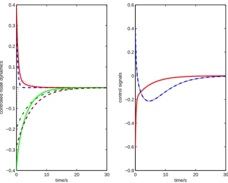
Example 1. Consider the following controlled time-varying complex dynamical network that is consisted of 2 non-identical, third-order nodes.
xx˙˙1112 ˙ x13 = x11+ x0 212 x11− x12 − 0.025 cos(t)A(t) xx1112 x13 + 0.025 cos(t)A(t) xx2122 x23 + e x12 ex12 0 u1, xx˙˙2122 ˙ x23 = −3x5x21− x23 23+ 3x223+ x21 x21− x323 + 0.03 sin(t)A(t) xx1112 x13 − 0.03 sin(t)A(t) xx2122 x23 + x20 22+ 1 0 u2, where A(t) = 1 + e −t 0 0 0 1 + e−2t 0 0 0 1 + e−3t .
A straightforward calculation yields: α1 = −2x12(x11+ x212)/(1 + 2x12) ex12,
β1 = −((1 + 2x12) ex12)−1, T1 : z11 = x13, z12 = x11 − x12, z13 = −x11− x212
and α2 = (x323− x23− x22)/(x222+ 1), β2 = −(x222+ 1)−1, T2 : z21 = x21, z22 =
0 10 20 30 −0.4 −0.3 −0.2 −0.1 0 0.1 0.2 0.3 0.4 time/s
controlled node dynamics
0 10 20 30 −0.8 −0.6 −0.4 −0.2 0 0.2 0.4 0.6 time/s control signals
Fig. 1. Evolution of state variables and control signals.
The first dynamical node can be stabilized by a feedback v1=−z11−2z12−3z13,
and the corresponding Lyapunov function is V (z) = zTP z with
P = 2.32.1 2.14.6 0.51.3 0.5 1.3 0.6 , W (t) = µ 1− 0.62|sin(t)|(1 + e−t) 0.62|sin(t)|(1 + e−t) 0.37|cos(t)|(1 + e−t) 1− 0.37|cos(t)|(1 + e−t) 
is positive definite for any t > 0, k1 = 1, k2 = 12.3654. The conditions of the
Theorem 3.1 are satisfied. Therefore, the above network can be stabilized by the following decentralized state feedback controller with holographic structure
u1=−2x 11x12− 2x312+ x13− x11− 3x212 (1 + 2x12) ex12 , u2=−4x 4 23+ 6x23+ 4x22− 6x21 −(x2 22+ 1) .
We choose the initial state as x0= (0.35, 0.4,−0.2, −0.3, −0.1, −0.28) and obtain
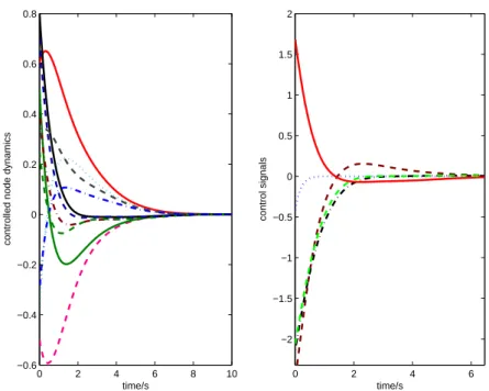
Example 2. Consider the following controlled time-varying complex dynamical network that is consisted of 5 identical second-order nodes.
µ ˙ xi1 ˙ xi2 ¶ = µ −xi2 − sin(−xi1+ 2xi2) ¶ + µ 0 1 ¶ u1 + 5 X j=1 cij(t) µ 2t+sin(t) t 0 0 1 ¶ µ xj1 xj2 ¶ , yi= xi1− 2xi2, i = 1, 2, . . . , 5, where we define C(t) = (cij(t))5×5, C(t) = 0.01×
−4 sin(t) sin(t) sin(t) sin(t) sin(t)
cos(t) −4 cos(t) cos(t) cos(t) cos(t) 3 sin(t) 3 sin(t) −12 sin(t) 3 sin(t) 3 sin(t) 3 cos(t) 3 cos(t) 3 cos(t) −12 cos(t) 3 cos(t) 4 sin(t) 4 sin(t) 4 sin(t) 4 sin(t) −16 sin(t)
Let ui = sin(−xi1+ 2xi2) + xi1− 2xi2= sin(yi)− yi, i = 1, 2, . . . , 5, V (z1, z2) =
3z12− 2z1z2+ z22. A direct computation gives: ri1(τ ) = ri2(τ ) = (2−
√ 2)τ2, i = 1, 2, . . . , 5, ki= 3, i = 1, 2, . . . , 5, ¯k = 7, W (t) = 3 0 0 0 0 0 3 0 0 0 0 0 3 0 0 0 0 0 3 0 0 0 0 0 3 +
−0.28|sin(t)| 0.07|sin(t)| 0.07|sin(t)| 0.07|sin(t)| 0.07|sin(t)| 0.07|cos(t)| −0.28|cos(t)| 0.07|cos(t)| 0.07|cos(t)| 0.07|cos(t)| 0.21|sin(t)| 0.21|sin(t)| −0.84|sin(t)| 0.21|sin(t)| 0.21|sin(t)| 0.21|cos(t)| 0.21|cos(t)| 0.21|cos(t)| −0.84|cos(t)| 0.21|cos(t)| 0.28|sin(t)| 0.28|sin(t)| 0.28|sin(t)| 0.28|sin(t)| −1.12|sin(t)|
is positive definite for any t > 0. The conditions of the Theorem 3.4 are satisfied. Therefore, the above network can be stabilized by the decentralized output feedback controller.
We choose the initial state as x0= (−0.5, 0.5, 0.6, −0.4, 0.4, 0.8, 0.3, −0.3, 0.25, 0.7)
and the simulation results are depicted in Figure 2.
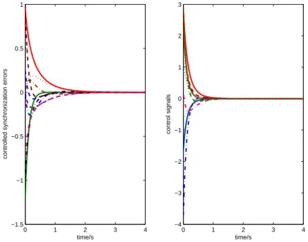
Example 3. Consider now a dynamical network that is consisted of 5 identical second-order nodes, which are described by
µ ˙ xi1 ˙ xi2 ¶ = µ 2 −3 3 5 ¶ µ xi1 xi2 ¶ + µ sin2(xi1)xi2 cos(xi2)xi1 ¶ + ui + 5 X j=1 cij(t) µ cos2(x i2) 0 0 1 ¶ µ xj1 xj2 ¶ , i = 1, 2, . . . , 5,
0 2 4 6 8 10 −0.6 −0.4 −0.2 0 0.2 0.4 0.6 0.8 time/s
controlled node dynamics
0 2 4 6 −2 −1.5 −1 −0.5 0 0.5 1 1.5 2 time/s control signals
Fig. 2. Evolution of state variables and control signals.
where we define C(t) = (cij(t))5×5, C(t) = 0.5×
5 sin(π/t) sin(t) e−t cos(t) e−2t sin(t) cos(t) cos(t) 5 sin(π/t) sin(t) e−t cos(t) e−2t sin(t) sin(t) cos(t) 5 sin(π/t) sin(t) e−t cos(t) e−2t cos(t) e−2t sin(t) cos(t) 5 sin(π/t) sin(t) e−t
sin(t) e−t cos(t) e−2t sin(t) cos(t) 5 sin(π/t) For the control design and computer simulation, the controller gain matrix and other parameter matrix are chosen as follows:
K(t) = µ −3 1 2 −4 ¶ , P (t) = µ 0.6406 0.2031 0.2031 0.5156 ¶ .
By direct calculation we have Q(t) µ 6 0 0 6 ¶ , W (t) =−0.4 ×
w11(t) |sin(t)|e−t |cos(t)|e−2t |sin(t)| |cos(t)|
|cos(t)| w22(t) |sin(t)|e−t |cos(t)|e−2t |sin(t)|
|sin(t)| |cos(t)| w33(t) |sin(t)|e−t |cos(t)|e−2t
|cos(t)|e−2t |sin(t)| |cos(t)| w44(t) |sin(t)|e−t
|sin(t)|e−t |cos(t)|e−2t |sin(t)| |cos(t)| w 55(t)
0 1 2 3 4 −1.5 −1 −0.5 0 0.5 1 time/s
controlled synchronization errors
0 1 2 3 4 −4 −3 −2 −1 0 1 2 3 time/s control signals
Fig. 3. Synchronization errors and control signals.
k¯h1(x, s, t)k2 ≤ 0.25|sin(π/t)|ke1k2 + 0.5|sin(t)|e−tke2k2 + 0.5|cos(t)|e−2tke3k2
+ 0.5|sin(t)|ke4k2+ 0.5|cos(t)|ke5k2,k¯h2(x, s, t)k2≤ 0.5|cos(t)|ke1k2+ 0.25|sin(π/t)|
ke2k2+ 0.5|sin(t)| e−tke3k2+ 0.5|cos(t)|e−2tke4k2+ 0.5|sin(t)|ke5k2,k¯h3(x, s, t)k2≤
0.5|sin(t)|ke1k2 + 0.5|cos(t)|ke2k2 + 0.25|sin(π/t)| ke3k2 + 0.5|sin(t)| e−tke4k2
+ 0.5|cos(t)|e−2tke5k2, k¯h4(x, s, t)k2 ≤ 0.5|cos(t)|e−2tke1k2+ 0.5|sin(t)|ke2k2+ 0.5
|cos(t)|ke3k2+ 0.25|sin(π/t)| ke4k2+ 0.5|sin(t)| e−tke5k2,k¯h5(x, s, t)k2≤ 0.5|sin(t)|
e−tke1k2 +0.5|cos(t)|e−2tke2k2+ 0.5|sin(t)|ke3k2+ 0.5|cos(t)|ke4k2+ 0.25|sin(π/t)|
ke5k2,k¯gi(xi, s, t)k2≤ keik2, λM(P (t)) = 0.7906, λm(Q(t)) = 6.
Thus W (t) is positive definite for all t > 0, where wii(t) = 11.05− 5|sin(π/t)|, i = 1, 2, . . . , 5.
It is readily seen above that the conditions of the Theorem 3.3 are satisfied. We choose the initial state as x0= (−0.5, 0.7, 0.45, −0.3, −0.45, 0.5, 0.45, 0.3, 0.2, −0.35)
and obtain the synchronization errors ei shown in Figure 3.
5. CONCLUSIONS
A representation model for a class of controlled time-varying complex dynamical net-works with similarity structure is proposed in this article. For this class of dynamical networks, the both decentralized state feedback and output feedback controllers with holographic-structure that asymptotically stabilize the network in closed loop are designed. Two stabilization criteria have been proved by using Lyapunov stability theory. Furthermore, the related synchronization problems were also investigated
hence several criteria for local and global network synchronization on the grounds of decentralized state feedback control were proposed too. In comparison with the relevant literature, the assumptions adopted to derive the presented main results are more general.
The proposed control designs are composed of a number of such sub-controllers, which not only possess decentralization but also the holographic property too. Each sub-controller possesses all the structural information of the others. More precisely, all sub-controllers share the same structure except for the different transformation parameters. Therefore once a sub-controller is designed, also all the others are obtained too. Practically, controllers with the same structure may be designed and thereafter adjusted by tuning some transformation parameters to create a family of controllers. An appropriate decentralized controller with holographic-structure in a given domain can be obtained this way. The control infrastructure is thus fairly easy to implement.
Three typical examples were explored and the respective computer simulations given. These demonstrate the effectiveness of the proposed control designs and the achievable performance. It should be noted, the effectiveness of the proposed method is even better exploited in cases with large node numbers.
ACKNOWLEDGEMENT
This work was partially supported by the NSF of P.R. of China, under the Grant No. 60574013, by Dogus University Fund for Science, and by Ministry of Education and Science of the Re-public of Macedonia. The authors would also like to acknowledge the anonymous reviewers whose critics helped considerably to improve the presentation quality.
(Received April 4, 2004.) R E F E R E N C E S
[1] A.-L. Barab´asi and R. Albert: Emergence of scaling in random networks. Science 286 (1999), 509–512.
[2] Changchun Hua, Xinping Guan, and Peng Shi: Decentralized robust model reference adaptive control for interconnected time-delay systems. J. Comput. Appl. Math. 193 (2006), 383–396.
[3] Chaohong Cai and Guanrong Chen: Synchronization of complex dynamical networks by the incremental ISS approach. Phys. A 371 (2006), 754–766.
[4] Chunguang Li and Guanrong Chen: Synchronization in general complex dynamical networks with coupling delays. Phys. A 343 (2004), 263–278.
[5] P. Erd¨os and A. R´enyi: On the evolution of random graphs. Publ. Math. Inst. Hautes ´
Etudes Sci. 5 (1959), 17–60.
[6] Guo-Ping Jiang, Wallace Kit-Sang Tang, and Guanrong Chen: A state-observer-based approach for synchronization in complex dynamical networks. IEEE Trans. Circuits and Systems. I Regul. Pap. 53 (2006), 2739–2745.
[7] Jianshe Wu and Licheng Jiao: Observer-based synchronization in complex dynamical networks with nonsymmetric coupling. Phys. A 386 (2007), 469–480.
[8] Jin Zhou and Tianping Chen: Synchronization in general complex delayed dynamical networks. IEEE Trans. Circuits and Systems. I Regul. Pap. 53 (2006), 733–744. [9] Jin Zhou, Junan Lu, and Jinhu L¨u: Adaptive synchronization of an uncertain complex
dynamical network. IEEE Trans. Automat. Control 51 (2006), 652–656.
[10] Jinhu L¨u and Guangrong Chen: A time-varying complex dynamical network model and its controlled synchronization criteria. IEEE Trans. Automat. Control 50 (2005), 841–846.
[11] K. Li and C. H. Lai: Adaptive-impulsive synchronization of uncertain complex dynam-ical networks. Phys. Lett. A 372 (2008), 1601–1606.
[12] D. J. Watts and S. H. Strogatz: Collective dynamics of small-world networks. Nature 393 (1998), 440–442.
[13] Xiao Fan Wang and Guanrong Chen: Pinning control of scale-free dynamical networks. Phys. A 324 (2004), 166–178.
[14] Xiao Fan Wang and Guangrong Chen: Synchronization in scale-free dynamical net-works: robustness and fragility. IEEE Trans. Circuits and Systems. I Regul. Pap. 49 (2002), 54–62.
[15] Xiaoqun Wu: Synchronization-based topology identification of weighted general com-plex dynamical networks with time-varying coupling delay. Phys. A 387 (2008), 997– 1008.
[16] Xiang Li and Guanrong Chen: Synchronization and desynchronization of complex dynamical networks: an engineering viewpoint. IEEE Trans. Circuits and Systems. I Regul. Pap. 50 (2003), 1381–1390.
[17] Xing-Gang Yan and Guan-Zhong Dai: Decentralized output feedback robust control for nonlinear Large-scale systems. Automatica 34 (1998), 1469–1472.
[18] Zhengping Fan and Guangrong Chen: Pinning control of scale-free complex networks. In: IEEE Internat. Symposium on Circuits and Systems, Madison 2005, pp. 284–287. [19] Zhi Li and Guanrong Chen: Global synchronization and asymptotic stability of com-plex dynamical networks. IEEE Trans. Circuits Syst. I Regul. Pap. 53 (2006), 28–33. [20] Zhi Li and Guanrong Chen: Robust adaptive synchronization of uncertain dynamical
networks. Phys. Lett. A 310 (2002), 521–531.
[21] ZhiHong Guan and Hao Zhang: Stabilization of complex network with hybrid impul-sive and switching control. Chaos Solitons Fractals 37 (2008), 1372–1382.
[22] Zhisheng Duan, Jinzhi Wang, Guanrong Chen, and Lin Huang: Stability analysis and decentralized control of a class of complex dynamical networks. Automatica 44 (2008), 1028–1035.
Wei-Song Zhong, Northeastern University, Shenyang, 110004. P.R. of China. e-mail: [email protected]
Jovan D. Stefanovski, HMS Strezhevo, MK-7000, Bitola. Republic of Macedonia. e-mail: [email protected]
Georgi M. Dimirovski, Dogus University, TR-34722 Istanbul, Republic of Turkey, and SS Cyril and Methodius University, MK-1000 Skopje. Republic of Macedonia.
e-mails: [email protected]
Jun Zhao, Northeastern University, Shenyang, 110004, P.R. of China, and Australian National University, Canberra ACT 0200. Australia.