ISSN 1450-288X Issue 19 (2011) © EuroJournals Publishing, Inc. 2011 http://www.eurojournals.com/JMIB.htm
Comparing Forecast Performances among Volatility Estimation
Methods in the Pricing of European Type Currency
Options of USD-TL and Euro-TL
Giray GozgorDepartment of International Trade and Business, Dogus University, Kadikoy, Istanbul, Turkey E-mail: [email protected]
Pinar Nokay
Economics, Istanbul University, Beyazit, Istanbul, Turkey
Abstract
By using the daily values of USD-TL and Euro-TL denominated European call and put option contracts, which are traded in the over-the-counter market, this study investigates whether there is a significant difference among the premiums of the contracts forecasted by historical volatility, EWMA(λ=0.94 andλ=0.97), GARCH(1,1) and E-GARCH(p, q) models. In order to test the significance of the difference among particular volatility series forecasted by these different methods, test techniques suggested by Diebold and Mariano (1995) and West (1996) are used.
Accordingly, the findings indicate that the differences in the pricing of the USD-TL and Euro-TL denominated call-put option contracts are statistically significant for some volatility forecasting methods.
Keywords: Option Pricing, European Type Vanilla Options, Historical Volatility,
Volatility Estimation Models, Forecast Comparison.
JEL Classcification Codes: G12, G17.
1. Introduction
The appearance of exchange rate risks dates back to 1973, when the Bretton Woods monetary system had been collapsed. It was after this date that it was needed to price the exchange rates in the market, and to measure and manage the exchange rate risk. Institutions and investors are easily protected from the appearance of exchange rate risk by derivative products such as forward agreements, futures contracts and options.
When we look at the variables of the used models in the pricing of the European type call or put option it can be seen that the variables, except the spot price volatility, constitute data. In this study, via the main historical volatility methods used in volatility calculations the option premiums have been calculated and it has been attempted to see whether or not there is significant difference among the option premiums calculated by different methods on a daily basis. At this point, the volatility estimation methods have not been taken as direct data however have been taken as part of the comparison by using European type options. In option contracts, the volatility is an important variable
in the estimation of the option premium and it has been observed that the methods of volatility for the option premiums have shown difference.
According to this, first of all, by taking into account the volatility estimation methods and the studies on volatility, the models used in the calculation of the option premiums written on the foreign exchange have been explained. Then, the theory behind these estimation methods have been specified and at the last section, is given the application.
2. Volatility Calculation Methods
In order to be able to calculate the price of the European Type option it is necessary to calculate the volatility according to a certain method. In general the volatility models which can be used in the pricing of options can be categorized in four main groups.
The concept of historical volatility includes volatility estimation methods such as moving average (MA) and exponentially weighted moving average (EWMA). However, historical volatility has a rather broad definition. E.g. Andersen et al. (2001) has handled the volatility observed in Multivariate VAR where there under the scope of historical volatility.
Another volatility estimation group is the GARCH models. ARCH (p), GARCH (p, q), E-GARCH (p, q) and other models which can be defined under these models. Each of these models has their own assumptions. Due to the difficulties to satisfy assumptions for option pricing models GARCH, E-GARCH and EWMA models are mainly used.
Stochastic Volatility (SV) is also another type of volatility estimation method. These models are models which introduce implied variances in place of the constancy estimation in the historical volatility. The most widespread SV models among these ones are the models developed by Hull and White (1987), Stein and Stein (1991) and Heston (1993).
One other volatility estimation group use in calculating option premium is the implied volatility method. Implied volatility differs from historical volatility as it aims to equalize the theoretical value calculated via past values of the basis asset on which the option is written with the option’s market value and it is a method in which the volatility calculation method aims further into the future.
2.1. Studies on Volatility Estimation
In general studies on volatility in the finance literature are based on the aforementioned four groups of volatility estimation methods and the comparisons made within themselves or with one other. In the literature, the studies which measure the estimation performance of the GARCH models have been done by Akgiray (1989), Pagan and Schwert (1990), Cumby et al. (1993), Duan (1995), Schmitt (1996), Figlewski (1997), Ritchken and Trevor (1999), and Duan and Wei (1999). These studies showed that GARCH, E-GARCH, EWMA, time series, stochastic volatility or implied volatility models can be effective for different assets in different interval time. Akgiray (1989), which is one of the studies on stocks and stock indexes has compared the EWMA, GARCH (1,1) and ARCH(2) models according to historical volatility and has reached the conclusion that the GARCH models showed effective performance. As for the studies on exchange rates, Andersen and Bollersev (1998) have compared the realized values of the one day later GARCH (1,1) estimations by taking the USD and the JPY-USD rates as a basis. Andersen et al. (1999), in their study where they used DM-USD Reuters quotations, have compared the volatility levels which have come into being according to certain time intervals with GARCH (1,1) volatility levels. These studies are those which conclude that GARCH (1,1) or similar models are accurate.
Dunis et al. (2000), in their expansive study on many of the exchange rates, have compared GARCH(1,1), implied volatility which they have calculated from forward rates, time series models, stochastic volatility models, and forward rates and they concluded that combinations which exist in EWMA are more accurate in volatility estimation. As for Lopez (2001), in the study performed on JPY-USD, DM-USD, GBP-USD, and the CAD-USD, has compared the performance of stochastic
volatility, EWMA, GARCH (p, q) and various time series models and has found that there is not a statistically significant difference between models. Pong et al. (2004), in their study on the GBP-USD, have compared estimations from various implied volatility values, time series models such as ARMA-ARFIMA and GARCH (1,1) and have inferred that significant conclusions had not been drawn from the all these models.
After these studies, in general, the combinations of the concerning four types of models have been subject to comparison. Studies by Andersen et al. (2006) and Becker and Clements (2008) have set example to studies which prove that the volatility models acquired via combinations are more accurate. As for Benavides and Capistran (2009), they have compared ARCH, GARCH (1,1), E-GARCH and various implied volatility combinations when working on the MXN-USD and have concluded that combinations which include ARCH models give more accurate results.
Some of the studies on volatility models in Turkey Markets have been done by Muradoglu and Kivilcim (1996), Yavan and Aybar (1998). Through these studies it has been inferred that different volatility models may be effective. Caglayan and Dayıoglu (2009) have recently determined GARCH models which may be most effective in OECD countries and have used the concerning values in the estimation of exchange rates. Thus, it has been concluded that the GARCH models are differently effective in every one of the countries. In addition it can be said that our study is the first study to use different volatility estimation models on exchange rate options pricing for comparison in Turkey Exchange Rate Markets.
2.2. Volatility Estimation Methods Used in the Study
In this study, GARCH (1,1), E-GARCH(p, q), EWMA(λ=0.94), and EWMA(λ=0.97) estimation models have been used.
2.2.1. GARCH (1, 1) Model
GARCH models have been introduced by Engle (1982) and have been expanded and generalized by Bollersev (1986). The GARCH (p, q) model has been defined by Bollersev (1986) as:
2 1 1 p q t i t i j t j i j h ω βh− α ε− = = = +
∑
+∑
(1)The ω>0 condition must exists in this model. Along with this in order for the ht value to be positive, it must be α≥ and β≥0 for GARCH (p, q). Also during the GARCH (p, q) process for the variance to be homoscedastic, the following assumption must exist:
1 1 1 p q i j i j β α = = + <
∑
∑
(2)In the GARCH (1,1) model the fact that the square of the expected errors of the yield of changes combined of estimations does not include the autocorrelation, and the assumption that it is random, are shown as below:
2 2
[
t]
t[
t]
tE
ε
=
h E z
=
h
(3)The main reason this model is used is that it responds quicker to the shocks than do the other models.
2.2.2. E-GARCH (p, q) Model
E-GARCH model, which is described as exponential GARCH, has been defined by Nelson (1991) as follows: 0 1 1 ln ln [ ( 2 / )] q p t j t j k t k k t k j k h α β h− θ ξ− γ ξ− π = = = +
∑
+∑
+ − (4)/
t th
tξ
=
ε
(5)The main difference between E-GARCH and GARCH is that in E-GARCH even if the conditional variance is negative the value of the parameter in question still can be evaluated logarithmically and due to this the variance will not always be positive. In these models ξ parameter t shows the asymmetric effects. Hence for the stationary of variance, the assumption below must be obtained: 1 1 q j j β = <
∑
(6)2.2.3. EWMA (Exponential Weighted Moving Average)
One other volatility model which takes place in this study is the EWMA model. Different from other moving average (MA) and the weighted moving average (WMA) and similar historical models reaches past data, although it is given less importance to in closer terms and this situation presents this model as a variance model dependent on exponential function:
2 t
σ
= 2 2 1 (1 ) 1 t Rt λσ− + −λ − (7) 2 tσ = Variance of the t day; 2 1
t
R− = Yield of the t-1 day; 2 1
t
σ− = Variance of t-1 day; λ = the
parameter of the chosen for weights (0 <λ< 1).
At this point λ is constant and generally is set as 0.94. Along with this JP Morgan has suggested an optimumλvalue to calculate volatility in certain countries with the EWMA method. For Turkey this value is 0.97.
In this study EWMA (λ=0.94), EWMA (λ=0.97), GARCH (1,1) and E-GARCH(p, q) volatility estimation models have been used. These models are the most frequently used ones for the trading exchange rates call and put options in the over-the-counter market. At this point it must be emphasized that the EWMA models are modeled by optimization and that the volatility estimation methods used by Balaban et al. (2006) are taken as basis.
3. Calculation of Option Premiums and Methodology
Whether the option contract is a call-put option or a European-American type option is an important effect on the option premium. Along with these facts there are also other variables which affect the option contract. These variables have modeled by Black and Scholes (1973) in order to price the European type option. Merton (1973) has also worked on a similar model in order to price the American type option in the same way.
Moving from the Black Scholes model other models for the pricing of options written on exchange rates have been developed. The most frequently used model among these ones is the Garman and Kohlhagen (1983) model. At the same time, the Grabbe (1983), Biger and Hull (1983) exchange rates option pricing model, which includes the forward rate and the bond interest variables, is also important. According to Chesney and Scott (1989), among these models, the Garman and Kohlhagen (1983) model is the most effective one, and thus in this study Garman and Kohlhagen (1983) model have been used.
There is an assumption that the spot price of the exchange rate on which the contract is written follows a stochastic process called the Wiener process, which is as follows:
dS= Sdt + Sdz
µ
σ
(8)Given that, in this equation S represents the concerning exchange rate’s spot price, µ represents the average, σ is the standard deviation, and dz is the random part which represents the Wiener process, Garman and Kohlhagen (1983) have showed the European type exchange call and put option premium as follows:
-r* -rt
C = Se tN(d1) - Ke N(d2) (9)
-rt -r*t
2 ln(S/K)+(r-r*+ / 2) 1 T d T σ σ = (11) d2 = d1 - σ T (12) In the formula;
C = Call option price; P = Put option price; S = Spot price; K = Strike price; r = Risk free domestic interest rate; r* = Risk free foreign interest rate; T = Day left until option’s maturity; σ = Volatility of the exchange rate’s spot price; N(d) = The probability of the area on the left of d given that the average is 0 and the standard deviation is 1 according to the normal distribution on the normal distribution table.
The domestic risk free interest rates used in the study are those of the shown internal benchmark Treasury bill in the concerning time interval for the options premium calculation time. As for the foreign risk free interest rates, they are the calculation of the daily average arithmetic mean of the benchmark Treasury bills within the given time interval according to the yield curve of 30, 60, 90 days introduced by the Nelson and Siegel (1987) method. The necessary data in order to do these calculations have been provided from Bloomberg. On the other hand, in the case that there has not been any trading on that day in the countries from where the data has been retrieved or in Turkey where there has not been any market trading on that day, the value of the day before would be issued as the value of that day. The same idea would go for the days on which there has not been any exchange rate trading in the Turkey Exchange Rate Markets.
The spot market price values used in the study are the free market values. Every one of the option premiums which have a daily value possess a one month maturity and their strike prices are accepted to be the forward rate value of every single day’s option contract. Since the aim of this study is the analysis of the effect of the difference among the volatility estimation models on the option premiums, and since there isn’t any organized stock market which can affect directly the premiums, the strike prices have been standardized. At this point, it must be emphasized that as the forward rate is the strike price both the call and put options will have the same value at different signs and in every one of the groups there will be the assumption that the spot price< the strike price.
Also, there isn’t an option market in Turkey where there can be done a comparison, and as there is a lack of premium value known as ‘realization’, the usage of methods, such as the mean error- ME, mean squared error- MSE, root mean squared error- RMSE, mean absolute error- MAE which give chance to calculate error estimation and to compute symmetric and asymmetric error statistics, can only be possible through taking the dynamic standard deviations as realized values. So, whether there is a statistically significant difference among the option premiums calculated via the these volatility models can only be computed by the help of tests which find differences between dynamic standard deviation values and option premiums.
4. Application
In this study, between the dates 01.01.2007 and 01.04.2009, by using daily values, the European type call and put option contract premium written on USD-TL and Euro-TL, has been calculated by using the Garman and Kohlhagen (1983) for different volatility estimation methods, all other variables held constant and standardized. Since 01.01.2007, a corporate tax is implemented on the income from future contracts and option markets trading, this is why this term is chosen as a beginning; as this situation may also increase the over- the-counter trading. Also, Hansen and Asger (2005), by using the GARCH(1,1) model, have limited the observation number, since the conditional variance values only give significant results up until 500 and if the observation number is greater than 500 other models which can observe the asymmetry due to more sensible measures must be used. Thus, there are 2016 options of which the premiums have been theoretically calculated consisting of 504 observations as USD (call and put) and Euro (call and put). The strike price is set as the forward rate, and due to this, the maturity difference among options has been made compatible.
4.1. The Estimation of the Volatility Values
Above, the GARCH (1,1), E-GARCH(p, q) and EWMA(λ=0.94) and EWMA(λ=0.97) models had been presented in a theoretical background, and these models have been used in the calculations of data within the given time interval. Meanwhile USD-TL and Euro-TL yields and the volatility values forecasted from mentioned models can be showed on graph.
Graph 1: USD-TL and Euro-TL yield values
Graph 2: USD-TL volatility values
0 0.050.1 0.150.2 0.250.3 0.350.4 0.450.5 0.550.6 04.01.07 04.05.07 04.09.07 04.01.08 04.05.08 04.09.08 EWMA (0.94)Year EWMA (0.97) Year
GARCH(1,1) Year EGARCH Year
Graph 3: Euro-TL volatility values
0 0.050.1 0.150.2 0.250.3 0.350.4 0.450.5 04.01.07 04.05.07 04.09.07 04.01.08 04.05.08 04.09.08 EWMA (0,94) Year EWMA (0,97) Year
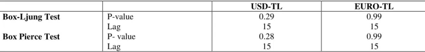
Firstly for testing the yields of exchange rates whether have on ARCH effect, optimum AR(p) and MA(q) process have been selected by Akaike Information Criteria (AIC) and Bayesian Information Criteria (BIC). It has been approved that selected AR (p) and MA (q) process have an ARCH effect. At this point it must be explained that in the GARCH (1,1) model the USD-TL and Euro-TL yield values have been analyzed for autocorrelation. The lag selection is taken as 15, the lag number suggested by Engle (2001). Hence, because the p value is greater than 0.05, there is no autocorrelation among the standardized error terms of sequential series. If, for the series where there is no autocorrelation GARCH (1,1) model is used, the conditional variance values resulted would be effective only up until 500 observations. Hansen and Asger (2005) suggested that any observation over 500 would need a more sensitive model which could measure the asymmetry. In this study 504 observations (worthy of two years) have been used, under the null hypothesis of there is no autocorrelation among series since there is no autocorrelation it has been concluded that the results will be consistent. According to this the autocorrelation results are as follows:
Table 1: GARCH (1,1) model autocorrelation test results
USD-TL EURO-TL
Box-Ljung Test P-value 0.29 0.99
Lag 15 15
Box Pierce Test P- value 0.28 0.99
Lag 15 15
In order to show that there is no autocorrelation within the series Q statistics can be used, to show that the specification of the variance equation is correct Q2 statistics can be used, and to show the ARCH effect on the selected lag in the variance equation ARCH-LM test statistics can be used. According to the ARCH-LM test which takes USD-TL and Euro-TL as a basis there is no remaining ARCH effect for both of the variables.
Table 2: GARCH (1,1) model Q and Q2 statistics
Euro-TL USD-TL
Lag AC PAC Q-Stat Prob. Lag AC PAC Q-Stat Prob.
0.016 0.1298 0.719 1 0.015 0.03 0.1538 0.497 2 0.01 0.01 0.18 0.914 2 -0.072 -0.059 0.18093 0.383 3 -0.078 -0.078 0.32518 0.354 3 0.032 0.034 0.18636 0.415 4 0.015 0.017 0.33604 0.499 4 0.108 0.13 0.24826 0.166 5 -0.028 -0.027 0.37702 0.583 5 -0.002 -0.025 0.24829 0.208 6 -0.085 -0.091 0.74977 0.277 6 -0.019 -0.012 0.25012 0.247 7 0.032 0.038 0.80181 0.331 7 0.019 0.032 0.2521 0.287 8 -0.02 -0.024 0.82209 0.412 8 0.017 -0.008 0.25359 0.332 9 0.044 0.032 0.92344 0.416 9 -0.045 -0.044 0.26444 0.331 10 0.007 0.015 0.92624 0.507 10 0.08 0.1 0.29836 0.231 11 0.077 0.067 0.12329 0.339 11 -0.035 -0.056 0.30496 0.248 12 0.013 0.012 0.12418 0.413 12 -0.035 -0.051 0.31167 0.264 13 0.07 0.076 0.14981 0.309 13 -0.025 0.001 0.31508 0.295 14 0.023 0.03 0.1526 0.361 14 0.009 -0.016 0.31556 0.34 15 -0.001 0.006 0.1526 0.433 15 -0.061 -0.085 0.33581 0.298
Lag AC PAC Q-Stat Prob. Lag AC PAC Q-Stat Prob.
1 0.056 0.056 0.15688 0.21 1 0.035 0.035 0.6166 0.432 2 -0.034 -0.038 0.21668 0.338 2 -0.051 -0.052 0.19182 0.383 3 -0.016 -0.012 0.22988 0.513 3 0.011 0.015 0.19831 0.576 4 -0.011 -0.011 0.23618 0.67 4 -0.004 -0.008 0.19909 0.737 5 -0.03 -0.03 0.28209 0.728 5 -0.015 -0.013 0.21088 0.834 6 -0.017 -0.015 0.29737 0.812 6 0.002 0.002 0.21103 0.909 7 -0.02 -0.021 0.31837 0.868 7 -0.048 -0.05 0.32972 0.856 8 0.014 0.014 0.32867 0.915 8 -0.029 -0.025 0.37435 0.879
Table 2: GARCH (1,1) model Q and Q2 statistics - (Continued). 9 0.002 -0.002 0.32889 0.952 9 0.067 0.064 0.60625 0.734 10 -0.013 -0.014 0.33771 0.971 10 -0.013 -0.019 0.61436 0.803 11 0.053 0.054 0.48182 0.94 11 -0.05 -0.043 0.74523 0.761 12 -0.001 -0.009 0.48183 0.964 12 0.002 0.001 0.74542 0.826 13 -0.053 -0.049 0.62876 0.935 13 0.06 0.057 0.93396 0.747 14 -0.016 -0.009 0.64161 0.955 14 -0.018 -0.022 0.95136 0.797 15 0.058 0.057 0.81431 0.918 15 0.042 0.046 0.10444 0.791
Table 3: ARCH-LM test results for USD-TL and Euro-TL
USD-TL (prob.) Euro-TL (prob.)
ARCH(1) 0.73 0.62
ARCH(2) 0.81 0.69
ARCH(12) 0.56 0.52
According to the results which have been achieved above, the estimated GARCH model coefficients are as follows:
Table 4: GARCH (p, q) model parameters estimation results
Variance Equation (USD-TL) Coefficient Std. Error z-Statistic Prob.
ω 0.000005 0.000001 3.412 0.0006
α 0.180893 0.031461 5.749 0
β 0.779609 0.035746 2.180 0
Variance Equation (Euro-TL) Coefficient Std. Error z-Statistic Prob.
ω 0.000004 0.000001 3.174 0.0015
α 0.149767 0.031321 4.781 0
β 0.817787 0.033626 2.432 0
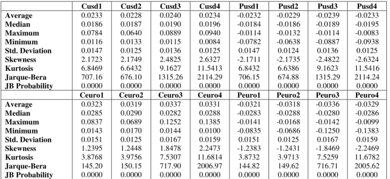
After the necessary conditions for models have been provided the option premiums for every one of the volatility models have been calculated. According to this, in Table 5 can be found the features of the series compounding of the call and put option values calculated via different volatility estimation methods, and the option premiums calculated via group one EWMA (λ=0.94), group two EWMA (λ=0.97), group three GARCH(1,1) and group four E- GARCH(p, q) are represented. The statistical features of these option premiums are shown as follows:
Table 5: Statistical Features of Daily Option Premiums
Cusd1 Cusd2 Cusd3 Cusd4 Pusd1 Pusd2 Pusd3 Pusd4 Average 0.0233 0.0228 0.0240 0.0234 -0.0232 -0.0229 -0.0239 -0.0233 Median 0.0186 0.0187 0.0190 0.0196 -0.0184 -0.0186 -0.0189 -0.0195 Maximum 0.0784 0.0640 0.0889 0.0940 -0.0114 -0.0132 -0.0114 -0.0083 Minimum 0.0116 0.0133 0.0115 0.0084 -0.0782 -0.0638 -0.0887 -0.0938 Std. Deviation 0.0147 0.0125 0.0136 0.0125 0.0147 0.0124 0.0136 0.0125 Skewness 2.1723 2.1749 2.4825 2.6327 -2.1711 -2.1735 -2.4822 -2.6324 Kurtosis 6.8469 6.6432 9.1627 11.5413 6.8432 6.6386 9.1623 11.5416 Jarque-Bera 707.16 676.10 1315.26 2114.29 706.15 674.88 1315.29 2114.24 JB Probability 0.0000 0.0000 0.0000 0.0000 0.0000 0.0000 0.0000 0.0000
Ceuro1 Ceuro2 Ceuro3 Ceuro4 Peuro1 Peuro2 Peuro3 Peuro4 Average 0.0323 0.0319 0.0337 0.0331 -0.0321 -0.0318 -0.0336 -0.0329 Median 0.0285 0.0290 0.0282 0.0288 -0.0283 -0.0288 -0.0280 -0.0286 Maximum 0.0837 0.0689 0.1252 0.1385 -0.0141 -0.0168 -0.0142 -0.0099 Minimum 0.0143 0.0170 0.0144 0.0100 -0.0835 -0.0686 -0.1250 -0.1383 Std. Deviation 0.0151 0.0125 0.0167 0.0159 0.0151 0.0125 0.0167 0.0159 Skewness 1.2395 1.2448 1.8478 2.2473 -1.2383 -1.2431 -1.8469 -2.2469 Kurtosis 3.8768 3.9756 7.5307 11.6814 3.8732 3.9713 7.5259 11.6782 Jarque-Bera 145.20 150.15 717.90 2006.97 144.82 149.62 716.71 2005.62 JB Probability 0.0000 0.0000 0.0000 0.0000 0.0000 0.0000 0.0000 0.0000
The outliers of the obtained option premiums have been left as are and no transaction has been made regarding the outliers. As it can also be seen in the yield graphs the USD-TL and the Euro-TL series are stationary. Stationary tests have also been done for the related series and it has been proved that the series are stationary. However, since only the volatility levels for the concerning days are needed for the comparison, there has been no need to show the obtained results. At this point it can be said that the average and standard deviation values found for both the call and put options remain the same. In order to reach this conclusion there has not been any need for the usage of techniques to test the difference among the averages, and from this point on, due to these obtained results, the call and put options will be observed together during the forecasting performance evaluation. Pong et al. (2004) showed that there could be significant impact on adding AR(p) and MA(q) terms into GARCH(p, q) equation so, this suggestion could not be applied because of assumptions did not satisfy the conditions for Turkey Options Exchange Markets. So ARMA-GARCH mixture could not add to this study. It is possible to draw from volatility graphics, starting 2008:09 data financial turmoil could have caused significant changes in volatility, we followed a structural breaks methods on GARCH (p, q) models suggested by Herwartz and Reimers (2002). Furthermore, unit root test allowing structural break test suggested by Zivot and Andwers (1992) was applied to data sets. It can be said that contrary to expectations, financial turmoil as a structural break has not a significant effect on all options premium.
4.2. Forecasting Performance Evaluation
Error statistics defined for forecasting are used in order to compare the models’ estimated values and the realized values by disregarding the sign of the differences and the magnitude of the estimated values and the realized rate values. The most frequently used forecast error statistics are the root mean square error (RMSE), mean square error (MSPE), and the mean absolute error (MAE) methods. During the comparison of the estimation models the values of RMSE, MAE, and MSPE must be smaller than the error statistics of an accurate model. Thus, error forecast statistics have been defined as follows:
RMSE= 2 2 1 1 1 1 ˆ ( ) N N t t t t t N = ε N = σ σ = −
∑
∑
(13) MSPE= 2 2 1 1 1 1 ˆ ( ) N N t t t t t N = ε N = σ σ = −∑
∑
(14) MAE= 1 1 1 1 ˆ N N t t t t t N = ε N = σ σ = −∑
∑
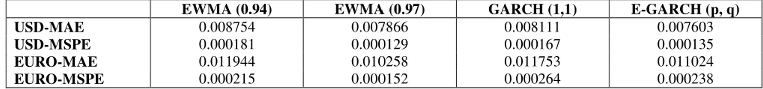
(15)According to the points mentioned above, the estimated performance values, calculated via the USD-TL and Euro-TL volatility values based on the concerning methods, have been found as follows:
Table 6: Volatility estimation performance evaluation results in the USD-TL and Euro-TL option premiums EWMA (0.94) EWMA (0.97) GARCH (1,1) E-GARCH (p, q)
USD-MAE 0.008754 0.007866 0.008111 0.007603
USD-MSPE 0.000181 0.000129 0.000167 0.000135
EURO-MAE 0.011944 0.010258 0.011753 0.011024
EURO-MSPE 0.000215 0.000152 0.000264 0.000238
Whether or not there is a significant difference among the obtained values can be measured via tests introduced by Diebold and Mariano (1995), West (1996), Clark and West (2007), which measure significant differences among values such as MSPE, RMSE, or MAE. Based on this in the study with the methods introduced by Diebold and Mariano (1995) and West (1996), it has been tested whether or not there is a significant difference among the option premiums’ MSPE values. In the study the Theil’s inequality coefficient has not been taken as criteria during the comparison. It must also be said that, in the study, for the comparison of the obtained volatility values, a dynamic forecasting (rolling window) has been made.
4.3. The Testing of the Difference among the Option Premiums
The test statistics of Diebold, Mariano and West (DMW) is as follows: H0: σ12−σ22 =0 H1: σ12−σ22 ≠0( 2 2 1 2 0 σ −σ > or 2 2 1 2 0 σ −σ < )
Based on this test statistics, firstly, one model is held fixed. In this study the model which is held fixed is the GARCH (1,1) model. According to this the MSPE value of the model held fixed is found as:
2 1 2 1 P (yt i)
σ −
+
=
∑
: Along with this MSPE value of the other model which will be compared with the fixed model is found as:2 1 2
2 P (yt i yˆt i)
σ −
+ +
=
∑
− : Precisely now it must be said that the value of yt i+ is deviated from thefixed model’s actual value and the yt i+ −yˆt i+ value shows the deviation from the other model’s actual value, to which will be compared. P is the observation number.
While the null hypothesis value shows that the performances of both the methods are equal, the alternative hypothesis shows that the other model explains more errors than does the fixed model, hence, it possesses worse forecast.
Based on the points above, the DMW test statistics have been defined as:
1 f DMW P V− = (16)
ˆ
(
)
t i t i t if
=
y
+−
y
+−
y
+ (17) 1 f =P−∑ and f V=P−1∑
( )f 2 (18)If the information provided above is implemented, the DMW test results of the calculated option premiums for the concerning volatility estimation methods are found as:
Table 7: The option premiums’ DMW test results according to the USD-TL and Euro-TL volatility methods GARCH (1, 1) EWMA (0.94) EWMA (0.97) E-GARCH (p, q)
Parity k MSPE MSPE DMW MSPE DMW MSPE DMW
TR-USD 504 0.000167 0.000181 -1.512 0.000129 0.588 0.000135 2.514**
TR-EURO 504 0.000264 0.000215 -0.352 0.000152 2.758*** 0.000238 3.502*** *Represents the 10%, ** 5%, ***1% significant level respectively
Based on this test’s statistical results on the option premiums and the call and put option premium contracts written on the USD-TL, which have been calculated via different estimation methods, there is no significant difference among EWMA(0.94)-GARCH(1,1), EWMA(0.97)-GARCH(1,1), EWMA(0.94)-EWMA(0.97), and the E-GARCH(p, q) method shows better performance in 5% significant level compared to the other methods. As for the option contracts written on the Euro-TL and the call and pull option contracts, the EWMA (0.94)-GARCH(1,1) methods do not present a significant difference, and the EWMA(0.97) and E-GARCH(p, q) shows better performance for a 1% significant level.
5. Conclusion
In the study, by using the daily values between the dates January 2007- January 2009, the European type call and put option contracts’ premiums written on the USD-TL and Euro-TL have been calculated based on the pricing model introduced by Garman and Kohlhagen (1983) and on different volatility estimation models; all other variables held constant. The possibility of a comparison among methods, which are used to calculate the volatility estimation models’ deviation and estimation values, has been calculated and performed. Differences among methods have been calculated via the test statistics introduced by Diebold, and Mariano (1995) and West (1996).
The selected models show similarities with the models suggested by Balaban et al. (2006). According to the results obtained, it can be said that there isn’t a significant difference between the EWMA (0.94) and the GARCH (1,1) models based on the Euro-TL and USD-TL contracts in the given term. As for the EWMA (0.97) model, it can be seen that this model, based on Euro contracts, shows significant difference when compared to the other models. As aforementioned, if the λ value presents a greater value, it means that the past values are given greater importance. When the past values become more important in the modeling, it has been observed that the EWMA model can show significant differences. During the term where these results were obtained, it is expected that the positive and negative volatility fluctuations which have been observed in the parity value of the USD-Euro, have been effective. Hence, the following conclusion can be drawn; the usage of EWMA (0.94) and GARCH (1,1) models according to the USD-TL and Euro-TL in the pricing of options in the Turkish Exchange Market and in the pricing of the European type options written on the USD-TL and Euro-TL by taking into consideration the given time interval, does not represent any significant difference. E-GARCH model is a best fitting model for pricing options Also that means USD-TL and Euro-TL exchange rates volatility shows the asymmetric effects.
On the other hand, since there is not yet an option market where the option contracts’ trading takes place in Turkey, it is not possible to make any comparisons by using the estimation models which would ordinarily be used via the options. The assumptions brought upon in this study must also be considered. The fact that the exchange options’ trading takes place in the over-the-counter market may cause the traders to move from historical volatility towards implied volatility. It is inevitable in the existing market conditions of today that the trader which defines the option premium (usually the seller of the option) will take into consideration their own internal situation as well as the market conditions in which are included the implied volatility, and will take into consideration the profit-loss one can make from the options, and will use these conditions for one’s own interest. Because, options which possess various strike prices and different premium values according to date do not exist. It has been observed that, within the changing market conditions the symmetric and asymmetric volatility models in the given time interval can present significant differences among results obtained during the usage of the pricing of exchange rates. Thus, based on the conception that these methods can substitute one other (at least until an organized market develops) it can be inferred that none of them should be used on a regular basis.
Acknowledgement
Giray Gozgor would like to thank Prof. Dr. Ertan Oktay for useful comments and suggestions.
References
[1] Akgiray, V., 1989. “Conditional Heteroskedasticity in Time Series of Stock Returns: Evidence and Forecasts”, Journal of Business, 62, p. 55–80.
[2] Andersen, T.G. and Bollerslev, T., 1998. “Answering the Skeptics: Yes. Standard Volatility Models Do Provide Accurate Forecasts”, International Economic Review, 39(4), p. 885–905. [3] Andersen, T.G., Bollerslev, T., and Lange, S., 1999. “Forecasting Financial Market Volatility:
Sample Frequency vis-à-vis Forecast Horizon”, Journal of Empirical Finance 6(5), p. 457–477. [4] Andersen, T.G., Bollerslev, T., Diebold, F.X. and Labys, P., 2001. “The Distribution of Realized Exchange Rate Volatility”, Journal of American Statistical Association, 96(453), p. 42–57.
[5] Andersen, T.G., Bollerslev, T., Christoffersen, P.F. and Diebold, F.X., 2006. Volatility and Correlation Forecasting Handbook of Economic Forecasting, Amsterdam, Elsevier.
[6] Balaban, E., Bayar, A. and Faff, R., 2006. “Forecasting Stock Market Volatility further International Evidence”. The European Journal of Finance, 122, p. 171-188.
[7] Becker, R. and Clemens, A.E., 2008. “Are Combination Forecasts of S&P 500 Volatility Statistically Superior?” International Journal of Forecasting, 24, p. 122-133.
[8] Benavides, G. and Capistran, C., 2009. “Forecasting Exchange Rate Volatility: The Superior Performance of Conditional Combinations of Time Series and Option Implied Forecasts”, Banco de Mexico Working Papers, 01-09.
[9] Biger, N. and Hull, J.C., 1983. “The Valuation of Currency Options”, Financial Management, 12, p. 24-28.
[10] Black, F. and Scholes, M., 1973. “The Pricing of Options and Corporate Liabilities” The Journal of Political Economy, 81(3), p. 637-659.
[11] Bollerslev, T., 1986. “Generalized Autoregressive Conditional Heteroskedasticity”, Journal of Econometrics, 31, p. 307–328.
[12] Caglayan, E. and Dayıoglu, T., 2009. “Forecasting Exchange Rate Returns Volatility with ARCH Models”, (In Turkish), Istanbul University Econometrics and Statistics E-Journal, 9(1), p. 1-16.
[13] Chesney, M. and Scott, L., 1989. “Pricing European Currency Options: A Comparison of the Modified Black-Scholes Model and A Random Variance Model”, The Journal of Financial and Quantitative Analysis, 24(3), p. 267-284.
[14] Clark, T.E. and West, K.D., 2007. “Approximately Normal Tests for Equal Predictive Accuracy in Nested Models”, Journal of Econometrics, 138(1), p. 291-311.
[15] Cumby, R., Figlewski, S. and Hasbrouck, J., 1993. “Forecasting Volatilities and Correlations with E-GARCH Models”, Journal of Derivatives, 1, p. 51–63.
[16] Diebold, F.X. and Mariano, R.S., 1995. “Comparing Predictive Accuracy”, Journal of Business and Economic Statistics, 13(3), p. 253-263.
[17] Duan, J.C., 1995. “The GARCH Option Pricing Model”, Mathematical Finance, 5(1), p. 13-32. [18] Duan, J.C.and Wei, J., 1999. ”Pricing Foreign Currency and Cross Currency Options under
GARCH”, Journal of Derivatives, 7(1), p. 51-63.
[19] Dunis, C.L., Laws, J. and Chauvin, S., 2000. “The Use of Market Data and Model Combination to Improve Forecast Accuracy”, Liverpool Business School Working Paper.
[20] Engle. R.F., 1982. “Autoregressive Conditional Heteroskedasticity with Estimates of the Variance of United Kingdom Inflation”, Econometrica, 50(4), p. 987–1007.
[21] Engle. R.F., 2001. “The Use of ARCH/GARCH Models in Applied Econometrics”, Journal of Economic Perspective, 15(4), p. 157-168.
[22] Figlewski, S., 1997. “Forecasting Volatility”, Financial Markets. Institutions and Instruments New York University Salomon Center Working Paper, 6(1), p. 1-88.
[23] Garman, M. and Kohlhagen S., 1983. “Foreign Currency Option Values”, Journal of International Money and Finance, 2, p. 231-237.
[24] Grabbe, O.J. 1983. “The Pricing of Call and Put Options on Foreign Exchange”, Journal of International Money and Finance, 2, p. 239-254.
[25] Hansen, P. and Asger, R.L., 2005. “A Forecast Comparison of Volatility Models: Does Anything Beat A GARCH (1,1)?”, Journal of Applied Econometrics, 20, p. 873-889.
[26] Herwartz. H. and Reimers, H.E., 2002. “Empirical Modeling of the DEM/USD and DEM/JPY Foreign Exchange Rate: Structural Shifts in GARCH-models and Their Implications”, Applied Stochastic Models in Business and Industry, 18, p. 3-22.
[27] Heston, S.L., 1993, “A Closed Solution for Options with Stochastic Volatility with Application to Bond and Currency Options”, Review of Financial Studies 6(2), p. 327–343.
[28] Hull, J.C. and White A., 1987. “The Pricing of Options on Assets with Stochastic Volatilities”, Journal of Finance, 2, p. 281-300.
[29] Lopez, J.A., 2001. “Evaluating the Predictive Accuracy of Volatility Models”, Journal of Forecasting, 20(2), p. 87–109.
[30] Merton, R.C., 1973. “Theory of Rational Option Pricing”, Bell Journal of Economics and Management Science, 4(1), p. 141-183.
[31] Muradoglu, Y.G. and Kivilcim, M., 1996. “Efficiency of the Turkish Stock Market with Respect to Monetary Variables: A Cointegration Analysis”, European Journal of Operational Research, 90, p. 566-576.
[32] Nelson, C.R. and Siegel, A.F., 1987. “Parsimonious Modeling Yield Curves”. Journal of Business, 60(4), p. 473-489.
[33] Nelson, D.B., 1991. Conditional Heteroskedasticity in Asset Returns: A New Approach, Econometrica, 59(2), p. 347–370.
[34] Pagan, A.R. and Schwert, G.W., 1990. “Alternative Models for Conditional Models for Conditional Stock Volatility”, Journal of Econometrics, 45(1), p. 267–290.
[35] Pong, S., Shackleton, M.B., Taylor, S.J. and Xu, X., 2004. “Forecasting Sterling/dollar Volatility: A Comparison of Implied Volatilities and AR(FI)MA Models”, Journal of Banking and Finance, 28, p. 2541–2563.
[36] Ritchken, P. and Trevor, R., 1999. “Pricing Options under Generalized ARCH and Stochastic Volatility Processes”, Journal of Finance, 54(1), p. 377-402.
[37] Schmitt, C., 1996. “Option Pricing Using E-GARCH Models”, ZEW-Centre for European Economic Research Discussion Paper, 96(20).
[38] Stein, E.M. and Stein, C.J., 1991. “Stock Priced Distributions with Stochastic Volatility. An Analytical Approach”, Review of Financial Studies, 4(4), p. 727–752.
[39] West. K.D., 1996. “Asymptotic Inference about Predictive Ability”, Econometrica, 64(5), p. 1067-1084.
[40] Yavan, Z.A. and Aybar, C.B., 1998. “Volatility on ISE”, (In Turkish), ISE Review, 2(6), p. 35-47.
[41] Zivot, E.D. and Andwers, W.K., 1992. “Further Evidence on the Great Crash the Oil Price Shock and Unit Root Hypothesis”, Journal of Business and Economic Statistics, 10(3), p. 251-270.