available online at www.ssbfnet.com/ojs
CO2 Emissions in India: Are the States Converging?
Ramesh Chandra Das, PhD
a,
a
Department of Economics, Katwa College, West Bengal, India
Abstract
The rapid industrialization process that had originated from England to foster a huge world population has almost reached its target and at the same time it has imputed a cost upon the world lives in terms of its by-product. The most alarming factor which is one of the components of the Green House Gases is the Carbon Di Oxide (CO2) the emission of which has grown over time in parallel way of industrial growth irrespective of the categories of the countries. The present study has tried to raise the issue in a micro level for the states of India that has experienced a shift in its economic policy paradigm in the name of economic liberalization in the period 1991-92. The aim of the present study is twofold-one is to examine whether the states are converging in CO2 emissions and the other is to study whether the states are getting unequal over time in this respect. The study observes that the states are insignificantly β converging and significantly σ converging for the period 1980-2000. Segregating the data for pre reform (1980-91) and post reform (1992-2000) periods the study further observes that the states are undoubtedly converging in the former period but diverging in the later period at least by the σ convergence. The study also found that there is growing concentration in CO2 emissions over post reform era which is a notion of interstate inequality.
Key Words: Industrialization, Economic reforms, CO2 emissions, β and σ Convergence, Herfindahl-Hirschman Index
© 2013 Beykent University
1. Introduction
The theme of the World Development Report of the year 1992 was “Environment and Development” and since the publication of this report the environmental concerns have started dominating the agenda for public policies of the developed as well as developing economies in the world. India is no longer an exception. The environmental problems are related to non judicious resource extraction on the one hand and the land degradation, water contamination and air
a
Corresponding author. The author is designated as Associate Professor in Economics of Katwa College. All the future
pollution on the other the result of which is the climate change that affects the civil society in terms of different natural calamities and health hazards. As a special interest to the present study the most important sources of air pollution are located in the life styles of the growing urban population whose motivating forces are the technological progress and industrialization that originated from the nineteenth century England. In fact, the population dynamics of the humans (anthropogenesis) is guided by the carrying capacity of the earth that in its turn depends on the level of knowledge to transform the Nature on the basis of Law of Thermodynamics. Pollution is a real threat to the nature if it crosses the limit of the carrying capacity or degradability capacity of the earth (Pearce and Turner, 1990). The magnitude of pollution today is the instance of crossing the human power over the nature’s healing power. Estimates show that by the year 2030 the urban population will be twice the size of rural population in the world. Developing country as a whole will grow by 160 per cent over this period whereas the rural population will grow by 10 per cent only. At the same time a significant proportion of population is depending on the agricultural sector which can cater only a given size of population. Therefore, rise in population puts pressure upon the rural economy that puts down the wage rate and as a result the rural urban wage gap rises that ultimately induced the rural labourer to move to the urban zone which magnified the extent of urbanization (Harris and Todaro, 1970).
Growth of urbanization leads to the formation of formal and informal sectors where the industrial activities are mostly carried out. Parallel to the growth of industrial activities there are some related changes in the life styles of the concerned people that produce economic goods in the one hand and economic bads as the byproduct on the other. The economic bads which are unavoidable with the consumption of goods are the components of Green House Gases that are mainly CO2 besides others. The existing literatures show that there is a direct relation between growth of output and carbon emission in the initial stages of production (Holtz-Eakin, and Selden, 1995, Essien, 2011, Ghosal and Bhattacharya, 2008, Halicioglu, 2009, Grossman and Krueger, 1991, Azomahou, et. al, 2006). This is the essence of inverted U shaped Environmental Kuznets Curve (EKC) (Andreoni and Levinson, 2001, Aldy, 2004, Dasgupta, et al, 2002, Dinda, 2004 & 2005).
The case of India is not an exception with respect to the effect of pollution upon growth of its gross domestic products. The present study has taken the attempt to search for interstate CO2 emissions over time and keeping the fact of economic liberalization that had been activated in the period 1991-92. It has been established by many researchers that the states were closer before such a major policy shift but after that they have experienced rising growth paths with a growing interstate disparity. Some states were growing much and some were lacking in different aspects of growth. The existing literatures showed different factors for explaining such a diverging trends among the states. For instance, to Bhaduri (2008) there is an inverse relation between growth rate and inequality particularly for the emerging countries like India and China. To him, maximum contributor to the growth paradigm in India is rise in the factor productivity in the unorganized sectors where employment has been reduced at a considerable rate that leads to the rise in inter-class inequality. The work by Dasgupta, et al (2000) deals with growth and inter-state disparity in India. The study of Ghosh, et al (1998) is a notable work on economic growth and regional divergence in India from 1960 to 1995. They have found that the Indian states have been diverging from each other over this period. In another paper,
Marjit and Mitra (1996) have shown that state wise divergence in India may be due to the inequality persisting in the openness to trade of different regions of the country (captured by the Trade Openness Index). In another piece of research Thangamuthu and Sankaran (2004) analyzed the inter-regional convergence or divergence in the context of industrial sector reform. They have observed that the industrial performance with reference to the all India level appears to be better than even the industrially developed states like Maharashtra, Gujarat, Tamil Nadu and West Bengal. The study of Das and Ray (2009) has pointed out that the states are facing disparity in the credit-deposit ratio over time in the reform period for the study period 1972-2002. The present study, thus, tried to highlight the levels of CO2 emissions (which are one of the indicators of industrial as well as aggregate output growth) across the states under different perspectives.
3. Data and Methodology 3.1 Objective of the Study
The study aims at examining two objectives. The first is whether the states are converging in CO2 emissions and the second is whether the states are getting unequal over time in this respect
3.2 Application of the Model
Since the secondary data available for Indian states in the CO2 emissions is for the period 1980 to 2000 so our study covers this particular period out of which the pre liberalization/reform period is 1980-1991 and the post liberalization period runs from 1992 to 2000. We have used the data estimated by Ghosal and Bhattacharya (op cit) for the same period which they derived from different global institutes along with Centre for Monitoring the Indian Economy (CMIE).
Primarily we have used the graphical presentation to have an overall view of the status of the states in CO2 emissions. Basic statistical tools are used to quantify the estimates. The convergence analysis of the states in CO2 emissions has been done in line with Barro and Sala- i-Martin (1992) on Beta () and Sigma () convergence. By the term convergence it means that the states with lower initial CO2 emission at the year 1980/1992 will grow at a faster rate
than the states with higher initial CO2 emissions and ultimately the poor states will catch up with the rich ones. That ultimate state of the economy is called the steady state or long run equilibrium. This particular type of convergence is known as Absolute convergence. The underlying logic behind the arrival to such single long run equilibrium is
that the rich states with higher initial CO2 emission level faces diminishing marginal returns to the emission compared to the poor states with low initial CO2 emission. Another assumption behind Absolute convergence is that the states are similar in other parameters like population growth, savings rates, depreciation rates, level of government spending on creation of social infrastructures etc but they differ with regard to the initial CO2 emission. Choice of the base period is an important issue in this context. Choosing the slump phase in a business cycle as base period may produce an exaggeration of growth rates that may distort the conclusion of the theory. In his work on the convergence of the Indian states Subrahmanyam (1999) suggested that the average of three to five years’ values of the variable as base period’s value may enable us to avoid this kind of problem. But the story regarding convergence does not end here
because of the fact that the states with higher initial CO2 emission will grow at slower rate than the states with lower initial CO2 emission does not necessarily imply that the cross-state dispersion of CO2 emission will tend to fall over time. Therefore, they have developed another form of convergence namely Sigma () convergence which means that
the coefficient of variation of CO2 emission of states would gradually decline over time.
We can test the absolute convergence by estimating the following regression model-
log (kit) = + (1-) log(ki,t-1) + uit ………...(1)
It can be rewritten as
log (kit/ ki,t-1) = - log(ki,t-1) + uit ……….…(2)
where and are constants respectively for intercept and slope with 0<<1 and uit is a regular disturbance term. In
this equation a positive sign of means absolute convergence. That is, growth rate of CO2 emission [log (kit/ ki,t-1)] is
inversely related to the initial CO2 emission (ki,t-1). It is also to note that is nothing but the slope of the emission
growth function. In other words = -dlog (kt/kt-1)/dlog (kt-1). Here also works as the notion of speed of convergence.
If we plot the data of each state’s growth rate and initial CO2 emission in a scatter diagram and fit a linear trend through these points then a downward trend will imply convergence of the states. The model of Convergence states
that the coefficients of variation of a variable across different states should be declining over time. We can express the concept of Convergence by means of the following regression equation
log (CV) = a + bt + ut ……….……….(3)
where a is intercept constant, b is the slope constant or growth rate of CV over time and u is the random disturbance term. If the sign of b is found to be negative and significant then we can say that the trend of CV is downward and that there is convergence among the states by the criterion of Convergence.
The interstate concentration of CO2 emissions that is one of the indicators of measuring inequality has been analyzed in line with the Herfindahl-Hirschman Index (HHI) which is expressed as the sum of squares of shares of CO2 emissions. That is
where si = xi/X, i = 1, 2,…..16. xi is the quantity of emission by ith state and X is the total quantity of emission by the
club of the 16 major states. The value of HHI varies from unity and 1/n. If there is monopoly or one state has the total CO2 emission then HHI takes maximum value of unity. In that case the state concentration is maximum. In the opposite case, if there are n numbers of identical states holding 1/n share of the emission then the value of HHI is 1/n. This is the lowest possible value of HHI.
4. State Scenario of CO2 Emissions
Keeping aside the debate of whether the developed countries are largely responsible for today’s global warming (which is mostly caused by CO2 emission) compared to the emerging or developing countries we specify our analysis to the major states of India as representatives of all the states of the country which are taken to be 16 in number as the club of these states constitute about 87-97 per cent of all India level of CO2 emission. It is highly realistic to take up the issue for our study as India is the only emerging country which lies in top 10 CO2 emitting countries in the world with low per capita income (Ghosal and Bhattacharya, op cit). It is, thus, highly desirable to study the inter-state status of CO2 emissions in India. One possible explanation to the issue is that the rising growth and disparity in income, as evidential from the literature, appeared after the period of economic liberalization in the country can be explained by means of the disparity in CO2 emissions by the states.
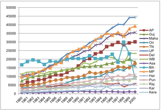
Figure 1: State wise CO2 Emissions (in metric tonnes)
Figure 1 highlights the total quantity of CO2 emissions by the states over time for the period 1980-2000. It is observed from the graphical presentation that almost all the states have followed rising trends in emission along with
0 5000 10000 15000 20000 25000 30000 35000 40000 45000 50000 AP Guj Maha Ori TN UP Del WB Asa Bih MP Har Pun Raj Kar Kera
their economic activities. There is a clear and persistent difference among the states that some of them have experienced steep rising in quantities of emission but the rest are in lower strata in this respect. The notable states which are following steep rise are Uttar Pradesh (UP), Madhya Pradesh (MP), Maharashtra, Andhra Pradesh (AP), Bihar and West Bengal (WB), although the state of Bihar has experienced downward trend after 1998 onwards. The states that lie in the lower panel in CO2 emission are Assam, Kerala, Haryana, Rajasthan and Delhi. Tamil Nadu (TN), Gujarat and Orissa are in the middle stage of the panel. It is commonly observed from the figure that the curves get steeper relatively after the major reform programmes starts in 1991-92 because of rise in economic activities in all fronts.
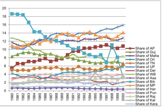
The difference tending to disparity among the states can be strongly observable when we look at the shares of CO2 emissions across the states. Figure 2 presents this situation. We observe that some states’ shares are rising but of some are falling. The top four states in quantities of emissions, viz. UP, MP, Maharashtra and AP are also maintaining rising shares along with Orissa, Rajasthan and Kerala. Bihar, WB, Gujarat, Delhi, Haryana and Assam are following the declining trends of emission. The steepest fall is observed for Bihar which is lacking in its position despite of having the BIMARU status that gave the special status by the central government to Bihar, MP, Rajasthan and UP regarding allocation of central development funds.
Figure 2: State wise shares of CO2 Emissions (in metric tonnes)
Hence, we find a perceptible difference among the states particularly after the inception of the reform process. But, prior to the reform process, the states are near closer to them. We, thus, need to examine whether the states are first converging or diverging and state concentration is falling or rising that will be answered in the following sections.
0 2 4 6 8 10 12 14 16 18 20 1 9 8 0 1 9 8 1 1 9 8 2 1 9 8 3 1 9 8 4 1 9 8 5 1 9 8 6 1 9 8 7 1 9 8 8 1 9 8 9 1 9 9 0 1 9 9 1 1 9 9 2 1 9 9 3 1 9 9 4 1 9 9 5 1 9 9 6 1 9 9 7 1 9 9 8 1 9 9 9 2 0 0 0 Share of AP Share of Guj Share of Maha Share of Ori Share of TN Share of UP Share of Del Share of WB Share of Asa Share of Bih Share of MP Share of Har Share of Pun Share of Raj Share of Kar Share of Kera
5. Convergence Test
As has been noted down in the methodology section that whether the states are converging or not can be examined in line with Barro and Sala- i-Martin (1992) Approach on Absolute Beta () and Sigma () convergence. Absolute convergence states that a state with low initial level of CO2 emission will grow in emission at a faster rate compared to the states that start with high levels of emission. The results of the said convergence will be found out in two ways-one is to plot all the sixteen combination of initial levels of emission and growth rates of emissions in a scattered diagram and compute the correlation coefficient of all the scattered points and test its significance. The test statistics is t = r √ (n-2)/√ (1-r2) ……….. (5)
for the Null Hypothesis: ρ = 0 against the Alternative Hypothesis: ρ ≠ 0, where ρ stands for population correlation and r stands for the sample correlation and (n-2 = 16-2 = 14) is the degrees of freedom. If the sign of correlation coefficient is negative and significant then it can be stated that the states are converging. Another way is to estimate Equation (1) or (2) and estimate the β coefficient and if it is found negative and significant then the states are said to be converging by means of absolute β convergence.
Another angle of convergence analysis can also be done by means of σ convergence where if it is found that the estimated regression coefficient of Equation (3) is negative and significant over time then we can say that the states are converging.
5.1 Absolute β convergence
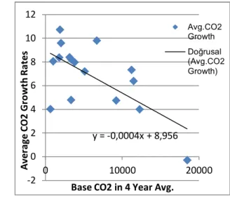
Figure 3 to 6 presents the scattered diagram of the coordinates of initial level of emission and annual average growth rates of emission over time with respect to different base levels and over different periods. For the entire period of study whether the base values of emission is of the year 1980 or the average values of first four year’s emission the sign of correlation coefficient is negative which are respectively -0.62 and -0.65 and significant. But the later base value gives stronger mode of convergence than the former (Table 1).
Figure 3: Absolute convergence (1980-2000) Figure 4: Absolute convergence (1980-2000)(4Yr)
y = -0,0004x + 8,8674 -2 0 2 4 6 8 10 12 0 10000 20000 Base CO2 in 1980 Avg.CO2 Growth y = -0,0004x + 8,956 -2 0 2 4 6 8 10 12 0 10000 20000 A ve ra ge C O 2 G ro w th R at e s
Base CO2 in 4 Year Avg.
Avg.CO2 Growth Doğrusal (Avg.CO2 Growth)
The difference in the results of single year base value and four year average base value shows the possibility of existence of divergence in any part of the total time length that is anticipated to lie in the post reform phase as the magnitude of correlation in the four year average value is greater.
Table 1: Correlation coefficients
Period/Base Emission 1980 as Base First 4 Yr. Avg. as Base
1980-2000 -0.62 -0.65
1980-91 -0.61 -
1992-2000 -0.18 -
Note: Bold figures stand for significance result at 5 % levels
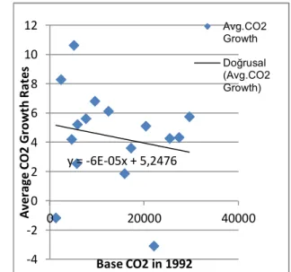
To assure this we have separated the absolute convergence analysis for the pre reform phase (1980-1991) from that of the post reform phase (1992-2000). The quantified results are given in Table 1. We observe from Figure 5 and 6 that the trend line across the scattered points in the former is steeper compared to the latter. The correlation coefficient for the pre liberalization period is high in magnitude and significant but that of the post liberalization period, although it is negative, but it is highly insignificant. It concludes that there is no question of divergence in CO2 emissions across the states in the pre liberalization period so far as the definition of absolute convergence is concerned. But there is no such convergence in the post reform phase by the same definition; instead there arises the possibility of divergence.
Figure 5: Absolute convergence (1980-91) Figure 6: Absolute convergence (1992-2000)
Let us estimate Equation (1) or (2) for finding the signs and magnitudes of in the entire periodical break ups. The results are presented in Equation (6) to (9).
Average Growth of CO2 (1980-2000) = 16.09 - 1.124 log base CO2 (1980) …….. (6) (t, p) = (2.86, 0.01) (-1.66, 0.11), R2 = 0.16 y = -0,0004x + 11,014 0 2 4 6 8 10 12 14 16 0 5000 10000 15000 20000 A ve ra ge C O 2 G ro w th R a te s Base CO2 in 1980 Avg.CO2 Growth Doğrusal (Avg.CO2 Growth) y = -6E-05x + 5,2476 -4 -2 0 2 4 6 8 10 12 0 20000 40000 A ve ra ge C O 2 G ro w th R at es Base CO2 in 1992 Avg.CO2 Growth Doğrusal (Avg.CO2 Growth)
Average Growth of CO2 (1980-2000) = 17.05 - 1.231 log base CO2 (4yr. Avg.) ……….. (7) (t, p) = (2.91, 0.01) (-1.75, 0.10), R2 = 0.18
Average CO2 Growth (Pre) = 19.76 - 1.33 log Base 1980 ………. (8) (t, p) = (3.3, 0.005) (-1.84, 0.08), R2 = 0.19
Average CO2 Growth (Post) = 6.79 - 0.26 log Base CO2 (1992) ……….. (9) (t, p) = (0.77, 0.45) (-0.27, 0.78), R2 = 0.0053
It is observed from the estimated equations that there is significant convergence in the pre liberalization period (the bold sign) and insignificant convergence in the post liberalization period (the parentheses represent the combination of t and probability values). The result for the entire period is insignificantly convergent with respect to 1980 as the base but significantly convergent when first four year’s emission is taken as base value. The poor values of R2 signify exclusion of other significant variables of explaining growth of CO2 emission.
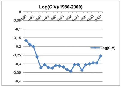
5.2 σ convergence
Let us now try to examine convergence among states by means of the definition of σ convergence. As we have noticed in the earlier sub section that the states are converging in the pre reform phase with no clear sign of convergence or divergence in the post reform phase. By σ convergence it is meant that the trend of logarithms of C.V should be falling and the regression estimate (Equation (3)) should be negative and significant. Doing the similar periodical break ups we observe from Figure 7 and Equation (10) to (12) that the states are unquestionably converging significantly during the pre reform phase as well as in the entire period but there is unambiguous and significant divergence result for the post reform phase.
Figure 7: σ convergence (1980-2000) log C. V (1980-2000) = -0.248 - 0.003 t ……….(10) (t, p) = (-12.31, 0.00) (-2.33, 0.03), R2 = 0.22 log C.V (1980-91) = -0.18 - 0.014t ………..(11) (t, p) = (-8.9, 0.00) (-4.95, 0.0005), R2 = 0.71 log C.V (1992-2000) = -0.429 + 0.007t ……….(12) (t, p) = (-11.47, 0.00) (3.40, 0.01), R2 = 0.62
Hence, we can conclude from the results of σ convergence that the states are converging during the pre liberalization and diverging in the post liberalization period in a significant manner that can match with other studies in the similar agenda.
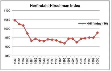
6. Measures of Concentration and Inequality
Let us now concentrate our analysis to the measurement of concentration of a few states in the distribution of CO2 emission by means of HHI index. The extract from the previous section is that the states are converging in the pre liberalization phase but diverging during the post liberalization phase so far at least the definition of σ convergence is concerned. By the help of Figure 2 and Equation (4) we have derived the HHI for the selected states of India which has been presented in Figure 8.
-0,4 -0,35 -0,3 -0,25 -0,2 -0,15 -0,1 -0,05 0 Log(C.V)(1980-2000) Log(C.V)
Figure 8: Measure of State Concentration of CO2 (1980-2000)
It is observed from the figure that up to the year 1991 the magnitudes of HHI are falling (which is the result of convergence) but after 1992 onwards the trend is upward sloping (because of divergence). Only a few states, notably, UP, MP, Maharashtra, Bihar, WB and AP are the leaders in emitting CO2 in India and thereby polluting the Indian as well as transboundary ambient environment. Hence, rise in CO2 emission leading to rise in industrial and other sectors’ production may be one of the factors behind rising growth and disparity in the Indian economy in the aftermath of the liberalization programme. It is, thus, prescribed to the pollution controlling authority in India to take measures against the highly polluting states to save the nation from the blame of the world nations and to relieve the low polluting states from the similar blame.
7. Conclusion
Based on the above analytical framework we are now in a position to conclude the entire study. We had started our journey under the view of examining two objectives of whether the states of India are converging and whether there is rising concentration of states over time, particularly after the reform when the measured variable is the quantity of CO2 emission. We have observed that the states are converging in a significant manner by both the definitions of β and σ convergence during the pre reform era but the states are unquestionably diverging with respect to the σ convergence only during the post reform era. It has been further observed that there is rising state concentration in CO2 emission after the year of reform. It is, thus, inferred from the study that the rising growth and disparity that were evidential from different studies in the reform period by means of different indicators can also be attributed to the levels of CO2 emissions as one of the leading growth determining factors.
References
Aldy, J. E. (2004). An Environmental Kuznets Curve Analysis of U.S. State - Level Carbon Dioxide Emissions, Department of Economics, Harvard University, Working Paper.
Andreoni, J. and Levinson, A. (2001). The Simple Analytics of the Environmental Kuznets Curve, Journal of Public
Economics, vol. 80(2), 269 - 286 850 900 950 1000 1050 1100 1 9 8 0 1 9 8 1 1 9 8 2 1 9 8 3 1 9 8 4 1 9 8 5 1 9 8 6 1 9 8 7 1 9 8 8 1 9 8 9 1 9 9 0 1 9 9 1 1 9 9 2 1 9 9 3 1 9 9 4 1 9 9 5 1 9 9 6 1 9 9 7 1 9 9 8 1 9 9 9 2 0 0 0 Herfindahl-Hirschman Index HHI (Indus)(16)
Azomahou T, Laisney F, Van Phu N. (2006). Economic development and CO2 emissions: a nonparametric panel approach. Journal of Public Economics 90, 1347–1363)
Barro, R.J and Sala-i-Martin (2004). Economic Growth, Second Edition, Prentice Hall of India Private Limited, New Delhi.
Bhaduri A. (2008). “Predatory Growth” a paper presented at the DRS sponsored two day conference on The Economics of Globalisation and Sustainable Development at the Department of Economics, Calcutta University, March 28-29
Das, R. C. and K. Ray (2009). Economic Reforms and Allocation of Bank Credit: A Sector-Wise Analysis of Selected States in Banking Sector Reforms – A Fresh Outlook, Mahamaya Publishing House, New Delhi
Dasgupta S, Laplante B. Wang H, Wheeler D. (2002). Confronting the environmental Kuznet’s curve. Journal of
Economic Perspective 16, 147–168
Dasgupta.D, P. Maiti, R. Mukherjee, S. Sarkar and S. Chakrabarty (2000). Growth and Inter-state Disparity in India,
Economic and Political Weekly, July 1-7
Dinda, S. (2004). Environmental Kuznets Curve: A Survey, Ecological Economics, vol.-49, 431-455
Dinda, S. (2005). A theoretical basis for the environmental Kuznets Curve, Ecological Economics, vol.-53, 403 – 413 Essien, A. V. (2011). The Relationship between Economic Growth and CO2 Emissions and the Effects of Energy Consumption on CO2 Emission Patterns in Nigerian Economy, Working Paper Series, Social Science Research Network, April, 13, http://papers.ssrn.com)
Ghosh, B, S. Marjit and C. Neogi (1998). Economic Growth and Regional Divergence in India: 1960 to 1995:
Economic and Political Weekly, June 27-July 3
Ghoshal, T and R. Bhattacharyya (2008). State Level Carbon Dioxide Emissions of India 1980 – 2000, Contemporary
Issues and Ideas in Social Sciences April 2008
Grossman, G. M., A. B. Krueger (1991). Environmental Impacts of a North American Free Trade Agreement. Working paper No. 3914, National Bureau of Economic Research
Halicioglu F. (2009). An econometric study of CO2 emissions, energy consumption, income and foreign trade in Turkey. Energy Policy 37(3), 1156–1164)
Harris, J. R and P. Todaro (1970). Migration, Unemployment and Development: A two sector analysis, American
Economic Review, 60
Holtz-Eakin, D. and T. M. Selden (1995). Stoking the Fire? CO2 emission and economic growth, Journal of Public
Economics, 57, pp 85 – 101)
Marjit, S. and S. Mitra (1996). Convergence in Regional Growth Rates: Indian Research Agenda: Economic and
Political Weekly, Aug 17-24
Pearce, D. W. and R. K. Turner (1990). Economics of Natural Resources and the Environment, Harvestor Wheatsheaf Subrahmanyam, S. (1999). Convergence of Incomes across States; a discussion paper, Economic and Political Weekly, Nov 20-26
Thangamuthu, C and A. Sankaran (2004). Industrial Sector Reforms: Tending Towards Inter-Regional Convergence or Divergence? Productivity, Vol. 45, No. 1