Artificial neural network based sparse channel estimation for OFDM systems

(1)

ARTIFICIAL NEURAL NETWORK BASED SPARSE CHANNEL

ESTIMATION FOR OFDM SYSTEMS

AbdurRehman Bin Tahir

2014.11.01.003

KADIR HAS UNIVERSITY

2017

(2)

AB DUR R E HM AN B IN T AH IR M .S . T he si s 20 1 7

(3)

ARTIFICIAL NEURAL NETWORK BASED SPARSE CHANNEL

ESTIMATION FOR OFDM SYSTEMS

ABDUR REHMAN BIN TAHIR

M.Sc., Electronics Engineering, Kadir Has University, 2017

Submitted to the Graduate School of Science and Engineering In partial fulfillment of the requirements for the degree of

Masters of Science in

Electronics Engineering

KADIR HAS UNIVERSITY 2017

(4)

(5)

ARTIFICIAL NEURAL NETWORK BASED SPARSE CHANNEL ESTIMATION

FOR OFDM SYSTEMS

Abstract

In order to increase the communication quality in frequency selective fading channel environment, orthogonal frequency division multiplexing (OFDM) systems are used to combat inter-symbol-interference (ISI). In this thesis, a channel estimation scheme for the OFDM system in the presence of sparse multipath channel is studied. The channel estimation is done by using the artificial neural networks (ANNs) with Resilient Backpropagation training algorithm. This technique uses the learning capability of artificial neural networks. By means of this feature we show how to obtain a channel estimate and how it allows the proposed technique to be less computationally complex; as there is no need for any matrix inversions. This proposed method is compared with the Matching Pursuit (MP) algorithm that is well known estimation technique for sparse channels. The results show that the ANN based channel estimate is computationally simpler and a small number of pilots are required to get a better estimate of the channel especially in low SNR levels. With this setting, the proposed algorithm leads to a better system throughput.

Keywords – Orthogonal Frequency Division Multiplexing (OFDM), Sparse Channel Estimation, Matching Pursuit Algorithm, Artificial Neural Network (ANN).

(6)

OFDM SİSTEMLER İÇİN YAPAY SİNİR AĞI TABANLI SEYREK KANAL

KESTİRİMİ

Özet

Frekans seçici sönümlemeli kanal ortamında, haberleşme kalitesini arttırmak için dik frekans bölmeli çoğullama (OFDM) sistemleri semboller arası girişimle baş edebilmek için kullanılmaktadır. Bu tezde, seyrek çok-yollu kanalın bulunması durumunda, OFDM sistemlerinde kanal kestirimi çalışılmıştır. Kanal kestirimi, Esnek Geri Yayılım eğitim algoritması kullanan yapay sinir ağları (YSA) ile gerçekleştirilmiştir. Bu teknik yapay sinir ağlarının öğrenme yetisini kullanmaktadır.Bu özellik sayesinde, kanal kestiriminin nasıl yapıldığı ve önerilen yöntemin herhangi bir matris tersine ihtiyaç duymadan daha az hesaplama karmaşıklığına nasıl sahip olabildiği gösterilmektedir. Önerilen bu yöntem, en uyguna yakın Eşleştirme Arama (MP) algoritması ile karşılaştırılmıştır. Sonuçlar, özellikle düşük SNR seviyelerinde daha iyi kanal kestirimi elde edebilmek için, YSA tabanlı kanal kestiriminin hesaplama kolaylığı sağladığını ve daha az sayıda pilot veriye ihtiyaç duyulduğunu göstermiştir. Böylece, önerilen yöntemin daha iyi bir sistem çıkışına olanak sağladığı gösterilmiştir.

Anahtar Kelimeler – Dik Frekans Bölmeli Çoğullama (OFDM), Seyrek Kanal Kestirimi, Eşleştirme Arama Algoritması, Yapay Sinir Ağları.

(7)

Acknowledgements

In the Name of Allah, the Most Beneficent, the Most Merciful. All the praises and thanks be to Allah, the Lord of the 'Alamin. To Allah everything belongs and to Him it shall return.

First, I would like to convey my earnest gratefulness to my advisor Dr. Habib Şenol and co-advisor Dr. Atilla Őzmen from Kadir Has University for their unremitting care during my M.S. study and research, for their endurance, inspiration, passion, and vast knowledge. They enlightened me through every step of the way and I could not have thought of having better advisors and mentors for my study. I am justly indebted to you sirs for all the help.

Further, I express my gratitude to my instructors for conveying the knowledge and insight throughout the Master’s program that made it possible today to finish and publish the work. Also, special thanks to my friends A. Ahad, A. Saad and M. Sohaib for their moral backing and for standing beside me through thick and thins of this long journey.

A final shout out to my brother and sisters, who associatively establish one of the strongest pillars on which this assembly stands today without a worry. This accomplishment would not have been possible without them. Thank you!

(8)

Dedication

To my parents...

(9)

List of Figures

Figure 1: (a) Multiple Carriers in FDM, (b) Multiple Orthogonal Carriers in OFDM ... 6

Figure 2: The basic block diagram of an OFDM system in AWGN channel ... 7

Figure 3: Wireless Multipath Channel ... 9

Figure 4: Sparse Multipath Channel ... 11

Figure 5: Time-Domain representation of the Sparse-multipath channel and its equivalent channel (𝜌𝜌 = 16) ... 13

Figure 6: Time-Domain representation of the Sparse-multipath channel and its DT equivalent channel (ρ=8) ... 14

Figure 7: Frequency-domain representation of sparse channel and its equivalent channel ... 14

Figure 8: Performance comparison for MP estimate, original and equalized channel (𝜌𝜌 = 𝛶𝛶 = 8) ... 19

Figure 9: Performance comparison for MP estimate, original and equalized channel (𝜌𝜌 = 20, 𝛶𝛶 = 8) ... 20

Figure 10: Performance comparison for MP estimate, original and equalized channel (𝜌𝜌 = 20, 𝛶𝛶 = 4) ... 21

Figure 11: Basic Structure of Biological Neuron ... 22

Figure 12: Structure of a simple Feed Forward ANN with R inputs, and S number of neurons in hidden layer ... 23

Figure 13: A Multi-Layer Feed Forward Network with 3 hidden layers ... 24

Figure 14: MLP-ANN model used with separate Real and Imaginary Inputs ... 29

Figure 15: Performance vector for multiple trainings ... 30

Figure 16: Neural Network model after training (nntraintool) ... 31

Figure 17: Performance comparison for ANN estimate, original and equalized channel (𝜌𝜌=8, 𝛶𝛶=8) ... 32

Figure 18: Performance comparison for ANN & MP estimate, original and equalized channel (𝜌𝜌=8, 𝛶𝛶=8) ... 34

Figure 19: Performance comparison for LMMSE-ANN & MP estimate, original and equalized channel (𝜌𝜌 = 𝛶𝛶 = 8) ... 35

Figure 20: Performance comparison for ANN & MP estimate, original and equalized channel (ρ=20, Υ=8) ... 36

Figure 21: Performance comparison for LMMSE-ANN & MP estimate, original and equalized channel (ρ=40, Υ=8) ... 37

Figure 22: Performance comparison for ANN & MP estimate, original and equalized channel (ρ=16, Υ=16) ... 38

Figure 23: MSE vs SNR comparison of MP and ANN based systems (𝜌𝜌 = 40, 𝛶𝛶 = 8) ... 39

Figure 24: MSE vs SNR comparison of MP and ANN based systems (𝜌𝜌 = 2, 𝛶𝛶 = 8) ... 39 vii

(12)

List of Tables

Table 1: ANN Parameters and Functions ... 31

Table 2: PC Resources and Capabilities ... 33

Table 3: Communication System's Parameters ... 33

Table 5: Complexity order of greedy (MP) algorithms for a given iteration ... 41

(13)

1. Introduction

In a general setup of wireless communication systems, a signal is transmitted which passes through a wireless medium and is received at the receiver. The wireless medium – generally called wireless channel – is modeled as a pseudo-differential operator. In data modulation sense, the basic communication systems modulate the data onto a single carrier frequency due to which the available bandwidth is completely occupied by the transmitted symbol. However, in modern communication systems, the available spectrum is divided into equal sub channels. This is the base of orthogonal frequency division multiplexing (OFDM), in which the sub channels are mutually orthogonal that helps in mitigating the inter-symbol interference (ISI) and hence, providing large data rates and radio channel impairments. The attraction of OFDM is due to the fact that it handles multipath effect at the receiver which causes ISI and frequency selective fading. In this communication setup, the wireless channel estimation refers to carefully calculating the operator and equalization refers to commuting the transmitted signal. In this thesis, we study the problem of channel estimation for OFDM in time-invariant sparse mobile communication channels. We use already established mathematical models to describe the signal and wireless communication channel. Our study largely focuses on the channel estimation part of the system; to devise an architecture that uses a more efficient and computationally les complex algorithm i.e. the artificial neural networks (ANNs) as channel estimators. Making use of the learning power of ANNs, a technique has been developed for channel estimation and the performance of this technique is studied. The performance – in terms of efficiency/correctness and computational complexity – of this suggested architecture is compared with the existing sub-optimal Matching Pursuit (MP) algorithm for the channel estimation under sparse setting.

(14)

Furthermore, not much work has been previously done on the implementation of the ANN as a channel estimator when the channel’s impulse response in the communication system is sparse. Another purpose that this study serves is the insight it provides to the channel estimation algorithms from the computational perspective. The Computational complexity theory is a separate field of study itself that is partly based on the theoretical computer science and mathematics; hence, studies have been done on the complexities of ANNs and MP algorithms. Making use of the proven theoretical models, we compare the time-complexities of both algorithms. Using the results from intense simulations in Matlab® environment, we show that given the right architectural parameters, ANN is superior than MP algorithm not just in terms of symbol error rate (SER) performance (information throughput) but is thought to be better in computational performance.

1.1. Literature Review

The wireless channels that occur just because of the multipath propagation of the transmitted signal and are static within one OFDM symbol are modeled with a convolutional operator i.e. the pseudo-differential operator reduces to a Fourier multiplier e.g. finite impulse response (FIR) filters. Such operators are perfectly diagonal in frequency domain and are known as frequency selective channels. Channel estimation of OFDM systems [1] in frequency selective channels with the help of pilot symbols are quite common [2] and is used in many applications. [3] discusses another approach of channel estimation by banded approximation of the channel matrix for OFDM systems. [4] and [5] discusses some optimal techniques for channel estimation and equalization and efficiency of the estimation algorithms. Some communication problems for OFDM contain channels with large delay spread and a smaller non-zero support [6]. These channels are known as sparse channels and are faced in a number of practical applications like high definition television (HDTV) where there are few echoes but the channel response spans hundreds of data symbols [7]. Some of the delay profiles like underwater acoustics or hilly terrain (HT) delay profile in broad-band wireless communication systems, comprise of a sparsely distributed multipath [8]. Different channel estimation techniques have been in use for such systems and proven to have

(15)

different performance under different settings; the properties of the Least Square’s estimators are investigates in [9]. An assemblage of sparse channel estimation algorithms has lately appeared and is known as compressed sensing [10]. Compressive sampling MP (CoSaMP) is used as sparse channel estimator in [11] based on the CoSaMP algorithm studied in [12]. The estimation of the channel taps one by one is done by using Matching Pursuit (MP) algorithm in [6] that is based on the work originally brought in light in [13].

However, all the mentioned multipath sparse channel estimation algorithms either suffer from an error floor or have high computational overhead. Artificial neural networks are computationally cheap and efficient algorithms that have caught much attention these days for channel estimation problems. In [14], authors have discussed an artificial neural network (ANN) based channel estimator that estimates the multipath channel in the frequency domain. The study uses multilayer perceptron NN (MLP-NN) with Levenberg-Marquardt as the learning algorithm.[15] evaluates the performance of pilot based OFDM system for multipath channel by using Generalized regression neural networks (GRNN) and adaptive network based fuzzy interference systems (ANFIS). A number of other studies use the same basic OFDM models and estimate the multipath channel either in frequency or time domain using ANN; with a slight change in the ANN architecture. [16] proposes a channel estimation using ANN for the LTE uplink system. Received pilot symbols are used in this study to first train the network and then estimate the whole channel. [17] – [19] also discuss the use of ANN as an estimator for OFDM systems under different assumptions. [20] – [21] are some further studies that make use of the recurrent neural networks (RNN) as channel estimator for different scenarios like multiple input multiple output OFDM (MIMO-OFDM) systems, STBC systems, OFDM interleave division multiple access (OFDM-IDMA) etc. A recent study [22] involves ANN based sparse channel estimation for MIMO-OFDM systems. [23] [24] [25] [26]

Computational complexity of the estimation algorithm is one of the major factors that define the quality of the estimator. Complexity theory being a separate field of study,

(16)

much effort has been made on the complexity analysis and comparison of diverse algorithms. A comparative complexity study on the several invariants of MP algorithm is done in [27] and [28]. The complexity of ANN, however, is still an open research question and a lot of effort has been made towards the satisfactory solution to this problem. The author in [29] argues that for neural networks, measuring the computing performance entails to new gears from information theory and computational complexity. The complexity of learning with regards to the Multi-Layer Perceptron ANN (MLP-ANN) is comprehensively discussed in [30] in which author ponders upon the expected computational complexity of the learning problem.

1.2. Research Methodology

The motivation behind this work was driven by the fact that with the advent of technology, the need to find better and easier ways to go from point A to point B has increased. This shows researchers a way of combining the classical algorithms with the advanced ones to find better and faster solutions. Under the umbrella of Digital Signal Processing in modern day’s wireless communications with high demand of bandwidth efficient algorithms, the channel estimation with better accuracy and efficiency becomes hard and computationally complex. This increase in complexity makes the machines’ ability to learn, an important factor that cannot be neglected. Various machine learning algorithms namely Artificial Neural Networks (ANNs), Support Vector Machines (SVMs) etc. have been previously used in some earlier studies for the purposes of channel estimation in different wireless communication settings. With this motivation, we formulate the research question of our thesis that which machine learning architectures can be used for channel estimation under sparse setting, and how? Further, to devise an architecture to find the algorithm that is more efficient and less computationally complex than the current sub-optimal algorithms.

This work answers the above questions and formulates a comprehensive solution to the given sparse problem. The author aims to extend this work to the case of Time-Varying Sparse Channels in which we observe a movement between the transmitter and

(17)

receiver; which in result introduces a phenomenon known as the Doppler’s effect. The channel estimation problem in this case becomes difficult, hence, more complex mathematical models and powerful channel estimation schemes are required in order to solve the said problem. Furthermore, the author believes that this work paves the way for the future work that can produce a better performing communication systems with lesser complexity. The use of ANNs impose some questions as the ANN optimization is still an open problem, so, with the advancements in the field of ANNs an optimized solution to such problems with lesser computational complexity and better communication system throughput can be obtained.

Firstly, this research aims to develop the system model in chapter 2, that includes the OFDM and channel properties and model derivations given in the successive sections. Thereafter, a matrix form of the channel model is also obtained towards the end of the chapter. Secondly, the fundamentals of channel estimation are discussed in chapter 3 that covers the classical estimation algorithms; the sub-optimal Matching Pursuit (MP) algorithm based sparse channel estimator that forms the benchmark for our study is discussed in the final subsections of the chapter. It continues into the chapter 4 with the introduction, working and architectural models for Artificial Neural Networks; where the ANN model for the proposed estimator’s architecture is discussed towards the end of the chapter. Finally, the results of this research obtained from simulations are presented and compared in Chapter 5 and conclusions are made in the final chapter 6.

(18)

2. System Model

2.1. Orthogonal Frequency Division Multiplexing (OFDM)

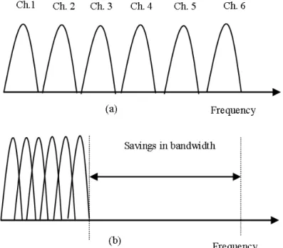
Before the advent of OFDM, FDM was used in order to transmit more than one signal through the telephone lines. As the name suggests, FDM divides the whole channel bandwidth into smaller sub-channels and multiple low rate signals are transmitted over the different sub-channels having different frequencies, fig. 1(a). However, this method is inefficient due to the fact that the sub-channels interfere with one another and have inadequacies even after being separated by a guard interval.

The urge to solve the bandwidth efficiency problem, gave birth to OFDM in which multiple, orthogonal, narrow-band sub-channels are transmitted in parallel hence, being more bandwidth efficient as pictured in fig. 1(b). Due to the demands of high data rates in wireless multimedia applications, OFDM has become more popular in recent times and becomes the modem of choice in modern wireless communication systems [31].

Figure 1: (a) Multiple Carriers in FDM, (b) Multiple Orthogonal Carriers in OFDM 6

(19)

Other than combatting with the multi-path fading and Inter-Symbol Interference (ISI), OFDM is also robust in high speed wireless communications. It is considered to be a remarkable method that is capable of decreasing the frequency-selective fading into flat fading by dividing the available bands into several subcarriers [32]. For this reason, OFDM symbol is quite longer than any other single-carrier system symbol, that makes it more robust against the delay dispersion of the channel and the fading caused by it [33].

2.1.1. OFDM Basics

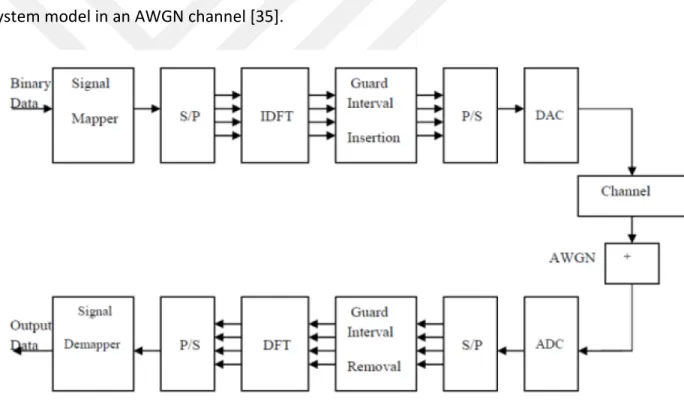
An OFDM signal is generated on the transmitter side digitally because of the difficulty in designing the signal and receiver in the analog domain [34]. Fig.2 shows a typical OFDM system model in an AWGN channel [35].

Figure 2: The basic block diagram of an OFDM system in AWGN channel

The incoming data stream is first modulated using any specific modulating schemes i.e. QPSK, QAM etc. and the symbol from these schemes are then serial to parallel converted. This parallel data is then fed to an N-point Inverse Discrete Fourier Transform (IDFT) and converted to the time domain sequence. IFFT is more cost efficient than IDFT, hence, is widely used as well.

(20)

The efficiency of OFDM lies in the fact that all the sub-carriers are closely spaced that is allowed because there exists orthogonality between them. This orthogonality can be checked by multiplying and then integrating any two subcarriers. Following section explain the signal model which hold the orthogonality principle for any given subcarriers. The carriers are linearly dependent if the carrier spacing is 1/𝑇𝑇𝑠𝑠𝑠𝑠𝑠𝑠, where 𝑇𝑇𝑠𝑠𝑠𝑠𝑠𝑠 is the

OFDM symbol duration; this can be held when the OFDM signal is defined by the FFT procedures. The OFDM symbol duration is defined as 𝑇𝑇𝑠𝑠𝑠𝑠𝑠𝑠 = 𝑁𝑁 × 𝑇𝑇𝑠𝑠, where 𝑁𝑁 is the

total number of subcarriers and 𝑇𝑇𝑠𝑠 is the sampling duration.

After the IFFT block, a cyclic prefix (𝐶𝐶𝐶𝐶) is added to the signal that helps to mitigate the ISI. 𝐶𝐶𝐶𝐶 is the copy of a fraction, typically 25%, of the last part of the individual OFDM symbol that is added to the start in order to allow the receiver to capture the starting point of the symbol with the probability of the length of 𝐶𝐶𝐶𝐶 [32].

2.1.2. Signal Model

We reflect an OFDM system with 𝑁𝑁 total subcarriers, the transmitted OFDM signal in discrete-time is then given as:

𝑠𝑠[𝑛𝑛] =_𝑁𝑁1�𝑁𝑁2−1 𝑑𝑑[𝑘𝑘]

𝑘𝑘=−𝑁𝑁₂ 𝑒𝑒𝑒𝑒𝑒𝑒(𝑗𝑗2𝜋𝜋𝑘𝑘 𝑛𝑛

𝑁𝑁) (1)

Where, N is the total number of sub-carriers, 𝑑𝑑[𝑘𝑘] is the frequency domain data symbol transmitted at discrete time 𝑛𝑛 and subcarrier 𝑘𝑘. By the Central Limit Theorem, 𝑠𝑠[𝑛𝑛] can be modeled as zero-mean complex Gaussian sequence, given that 𝑁𝑁 is sufficiently large [36]. A set of known data symbols with known locations – branded as pilot symbols – are also imbedded in the transmitted signal. These uniformly-spaced pilot symbols are used on the receiver side in channel estimation step and, hence, estimation is called Pilot-Aided channel estimation. Throughout this study, the symbol Υ will be used to represent the pilot spacing, hence, greater the value of Υ, smaller will be the total number of pilot symbols. The total number of pilot symbols are denoted by 𝑁𝑁𝑝𝑝.

(21)

After the CP insertion of length 𝐿𝐿𝑐𝑐, the multiple OFDM symbols are now ready to be

transmitted over consequent sub-carriers. These are then parallel to serial converted and transmitted over the Time-Invariant sparse multipath channel.

2.2. Wireless Channel

Ideally, the wireless channel should leave the transmitted signal unchanged so that the received signal equals the transmitted signal, i.e.𝑦𝑦(𝑡𝑡) = 𝑠𝑠(𝑡𝑡′), where 𝑡𝑡′_{= 𝑡𝑡 − 𝜏𝜏}

0 defines

the time shift equivalent to the time 𝜏𝜏0 it takes for the signal to reach the receiver from

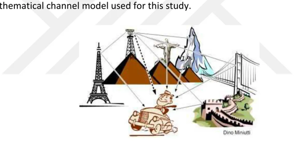
the transmitter. The ideal channel never happens in the practice obviously, hence, this subsection gives a brief review of some important properties of the wireless channel and its effect on the signal once it propagates through the channel. It also discusses the mathematical channel model used for this study.

Figure 3: Wireless Multipath Channel 2.2.1. Multipath Fading

The transmitted signal is affected by a number of factors while it propagates through the wireless medium. Firstly, electromagnetic waves deteriorate as it passes through the radio channel and the power of the received signal is decreased with the increased distance between the transmitter and receiver; known as path loss. Additionally, as the signals’ direct line of sight (LOS) path might be blocked by some physical objects, it might take other paths to the receiver; fig. 3 [37]. This multipath propagation occurs where the single transmitted signal arrives at the receiver through multiple different paths with different delays and attenuation factors because of the reflection, diffraction, scattering

(22)

etc. instigated by the physical objects (collectively assumed as Scatterers). This makes the received signal’s power fluctuate over time/frequency and is called fading. This multipath fading comes under the umbrella of small-scale fading and can be defined by the Rayleigh statistical model.

The communication problems concerning the estimation and equalization of the communication channels, that have a larger delay spread and small non-zero support, are being studied. These channels are known to have sparse channel impulse response. Sparse multipath channels (SMPC) can be seen in many real-world applications and the immobile channel impulse response in continuous time is written as:

𝑐𝑐(𝑡𝑡) = ∑𝐿𝐿−1𝑙𝑙=0𝛼𝛼𝑙𝑙𝛿𝛿(𝑡𝑡 − 𝜏𝜏𝑙𝑙) (2)

for 𝑙𝑙 = 0, … , 𝐿𝐿 − 1. where,

L is the total number of multi-paths 𝛼𝛼𝑙𝑙 is the attenuation factor for each path

𝜏𝜏𝑙𝑙 is the delay for the path 𝑙𝑙

The 𝛼𝛼𝑙𝑙 are a subset of complex natural distribution with zero-mean and variance of 𝜎𝜎𝑙𝑙2

i.e. ~ 𝒞𝒞𝒞𝒞(𝟎𝟎, 𝜎𝜎𝑙𝑙2 ) with normalized unit power.

As a sparse problem, it is not possible to directly show the discrete-time equivalent of (2), hence a discrete-time sparse representation is developed in the next section.

2.2.2. Sparsity in Wireless Channels

Given the fact that the transmitter, receiver and all the scatterers are static, the system can be modeled as linear time-invariant (LTI) system. Considering this, some communication environments involve channels with large delay spread and a small non-zero support; such problems occur quite often in practical implementations. The channel response of such channels spans many hundreds of data symbols in HDTV where there are a very few numbers of echoes due to multipath. The theory of LTI-SMPC suggests that 𝐿𝐿 << 𝑁𝑁𝐶𝐶𝐶𝐶, where 𝑁𝑁𝐶𝐶𝐶𝐶 is the length of the cyclic prefix (CP). An illustration of sparse

(23)

multipath channel i.e. 𝑐𝑐[𝑛𝑛] ≠ 0 for really limited values of 𝑛𝑛, is given in Fig. 4. The channel length in the figure is 40, however, the non-zero or dominant taps amount to 15.

Figure 4: Sparse Multipath Channel

Recently, Compressive Sensing (CS) technique has gained popularity because of its efficiency in signal acquisition frameworks where the signal considered as sparse or compressible in frequency or time-domain; meaning that for continuous signals, the information rate is much smaller than as depicted by the signal’s bandwidth. Also, a discrete-time signal relies on a certain degree of freedom that is fairly smaller than the signal’s finite span [38]. As a result, length of the training sequence can be shortened as compared to linear estimation techniques. CS explores the sparsity of the signals and it has shown to be possible because an exact depiction of such signals is possible in terms of a suitable basis.

Working on the discrete-time sparse signals is common as it is simpler than its continuous-time counterpart and also that it is more developed. Taking the Fourier transform (FFT) of CIR given in (2), we get:

(24)

𝐻𝐻(𝑓𝑓) = ∫𝑇𝑇𝑠𝑠𝑠𝑠𝑠𝑠𝑐𝑐(𝑡𝑡)𝑒𝑒−𝑗𝑗2𝜋𝜋𝜋𝜋𝜋𝜋_{. 𝑑𝑑𝑡𝑡}

0 (3)

Replacing (2) in (3) and simplifying the equation gives:

𝐻𝐻(𝑓𝑓) = ∑𝐿𝐿−1𝑙𝑙=0𝛼𝛼𝑙𝑙𝑒𝑒−𝑗𝑗2𝜋𝜋𝜋𝜋𝜏𝜏𝑙𝑙 (4)

where, 𝑓𝑓 = (−𝑁𝑁₂+ 𝑘𝑘)∆𝑓𝑓 for 𝑘𝑘 = 0,1, … , (𝑁𝑁 − 1) and ∆𝑓𝑓 = _𝑇𝑇1

𝑠𝑠𝑠𝑠𝑠𝑠; ∆𝑓𝑓 being the carrier

spacing and 𝑇𝑇𝑠𝑠𝑠𝑠𝑠𝑠 is the symbol duration. Also, the continuous-time path delays 𝜏𝜏𝑙𝑙 can

be represented in discrete-time, with a resolution factor 𝜌𝜌, as 𝜏𝜏𝑙𝑙 = 𝜂𝜂𝑙𝑙′(𝜌𝜌𝑇𝑇𝑠𝑠′); here, 𝜂𝜂𝑙𝑙′×

𝜌𝜌 = 𝜂𝜂𝑙𝑙 . Similarly, 𝑇𝑇𝑠𝑠𝑠𝑠𝑠𝑠 = 𝑁𝑁(𝜌𝜌𝑇𝑇𝑠𝑠′) and 𝑇𝑇𝑠𝑠 = 𝜌𝜌𝑇𝑇𝑠𝑠′. Then (4) can be written in simplified

form as:

𝐻𝐻(𝑘𝑘) = ∑𝐿𝐿−1𝑙𝑙=0𝛼𝛼𝑙𝑙𝑒𝑒−𝑗𝑗2𝜋𝜋(−

𝑁𝑁

2+𝑘𝑘)(𝜌𝜌𝑁𝑁𝜂𝜂𝑙𝑙) (5)

Eq. (5) represents the channel frequency response for the sparse channel impulse response given in (2). Now, in order to get the equivalent representation of discrete channel impulse response ℎ𝑒𝑒𝑒𝑒[𝑛𝑛], we take inverse Fourier Transform (IFFT) of (5) as:

ℎ𝑒𝑒𝑒𝑒[𝑛𝑛] = � 𝐻𝐻[𝑘𝑘] 𝐾𝐾 2−1 𝑘𝑘=− 𝑘𝑘₂ 𝑒𝑒 𝑗𝑗2𝜋𝜋𝜋𝜋𝑘𝑘 𝜌𝜌𝑁𝑁 (6)

After replacement and rearrangement of (6), we get the discrete time equivalent channel impulse response representation of the multipath channel. We can write it in matrix form as 𝒉𝒉𝒆𝒆𝒆𝒆= 𝑭𝑭𝜼𝜼† 𝑯𝑯, where, 𝑯𝑯 is given in (5) and 𝑭𝑭𝜼𝜼† ∈ ℂ𝜌𝜌𝑁𝑁𝐶𝐶𝐶𝐶×𝑁𝑁 is inverse of 𝐹𝐹𝜂𝜂 =

1 𝜌𝜌𝑁𝑁𝑒𝑒

−𝑗𝑗2𝜋𝜋_{𝜌𝜌𝑁𝑁}𝑘𝑘(𝑛𝑛−𝜂𝜂𝑙𝑙)_{and 𝑁𝑁}

𝐶𝐶𝐶𝐶 is the length of CP. The equivalent representation of channel’s

frequency response is then given as: 𝑯𝑯𝑒𝑒𝑒𝑒= 𝑭𝑭𝜼𝜼 𝒉𝒉𝒆𝒆𝒆𝒆 ∈ ℂ𝑁𝑁×1. 𝒉𝒉𝒆𝒆𝒆𝒆 will be used during the

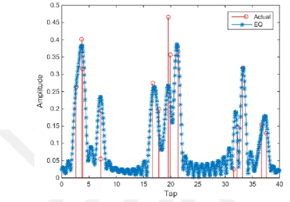
training part of neural networks as the target set. It is explained in detail in Chapter 4. The multipath sparse channel with 15 multipath was shown in fig. 4; its equivalent discrete time-domain representation 𝒉𝒉𝑒𝑒𝑒𝑒 with resolution 𝜌𝜌 = 16 is presented in fig. 5.

(25)

Figure 5: Time-Domain representation of the Sparse-multipath channel and its equivalent channel (𝜌𝜌 = 16)

The total number of multipath used for this study is 3 and fig. 6 presents the sparse multipath channel and its equivalent discrete time representation. The ripples that can be observed in the plots are due to the 𝑠𝑠𝑠𝑠𝑛𝑛𝑐𝑐 functions that arise because of the band-limited property of the channel. Also, as we can see that most of the values are either zero or near zero, such points are not required to be estimated and are mostly ignored at the channel estimation step by using a threshold factor. This is the reason why we require lesser pilots symbols for estimation and in return the throughput is increased.

(26)

Figure 6: Time-Domain representation of the Sparse-multipath channel and its DT equivalent channel (ρ=8)

Thus, the frequency domain representation 𝑯𝑯 and 𝑯𝑯𝑒𝑒𝑒𝑒 of 𝒉𝒉 and 𝒉𝒉𝑒𝑒𝑒𝑒, respectively, is

presented in the following Fig. 7.

Figure 7: Frequency-domain representation of sparse channel and its equivalent channel 14

(27)

We’ll see in the channel estimation sections that the resolution plays an important role in the efficiency of the estimation algorithm. Algorithms like MP that exploit the sparsity of the signal show difference in the performance on the basis of different values of 𝜌𝜌. The effect of 𝜌𝜌 can be observed by comparing figures 5 and 6.

2.3. Unaccountable Additive Noise

Other than the fading effects on the propagating signals, there are some other minor electromagnetic effects that are unaccountable for in the channel. The combination of these effects are catered for by adding a noise into the signal when it passes through the channel. The noise process is usually additive and is categorized by its intensity and distribution. The noise process is measured in Signal to Noise Ratio (SNR) which is a ratio, hence, have no units and is represented in term of decibels dB. In the frequency modulation techniques, SNR is usually measured as the ratio of the Energy per Bit to the Noise Spectral Density (Eb/N0). Being a process of noise, additive noise has zero as its first moment and the color of the noise is shown by its second moment. From the several statistical models, commonly used noise process is the Additive White Gaussian Noise (AWGN); with Gaussian being its distribution and White means that the white light is also a noise process, hence, affects the signal. In this thesis, we will use AWGN as the noise process with zero-mean and variance of N0 and will be represented in the following sections with w[-] in time domain and with W[-] in frequency domain.

2.4. Observation Equation

At the receiver, after removing the 𝐶𝐶𝐶𝐶 i.e. discarding the samples falling in the 𝐶𝐶𝐶𝐶 and symbol rate sampling, the received signal at the input of the Fast Fourier Transform (FFT) can be expressed as:

𝑦𝑦[𝑛𝑛] = �𝐿𝐿−1_𝑙𝑙=0𝑠𝑠[𝑛𝑛 − 𝑙𝑙]𝑐𝑐[𝑙𝑙] + 𝑤𝑤[𝑛𝑛] (5) Where, n=0, 1…, N-1. 𝑤𝑤[−] is the zero mean complex additive white Gaussian noise with variance 𝑁𝑁0.

(28)

The above input-output relationship is further evaluated and converted to a matrix form in order to apply a suitable channel estimation algorithm.

The input-output model of the signal can now be represented in a matrix form. The matrix form of the model makes it easier to represent the input-output relationship and use it for the further evaluation of the relationship in the channel estimation steps. As our problem belongs to the wider sparse representation problem, hence, according to the channel representation discussed in section 2.2, we can represent our observation model given in (5). Eq. (5) can be written in matrix form as:

� 𝑦𝑦(0)⋮ 𝑦𝑦(𝑁𝑁 − 1)� = � 𝑠𝑠(0) ⋯ 𝑠𝑠(−𝑀𝑀 + 1) ⋮ ⋱ ⋮ 𝑠𝑠(𝑁𝑁 − 1) ⋯ 𝑠𝑠(𝑁𝑁 − 𝑀𝑀) � � 𝑐𝑐(0) ⋮ 𝑐𝑐(𝑀𝑀 − 1)� + � 𝑤𝑤(0) ⋮ 𝑤𝑤(𝑁𝑁 − 1)� (6) Which can be condensed to:

𝒚𝒚 = 𝑨𝑨𝑨𝑨 + 𝒘𝒘 (7)

From eq. (7), it is known that the channel is sparse and the problem is to approximately calculate the received vector 𝒚𝒚 in terms of a linear combination of a small number of columns from the matrix 𝑨𝑨. In other words, we must find 𝑨𝑨 in (6) such that 𝒚𝒚 ≈ 𝑨𝑨𝑨𝑨 [6]. The matrix 𝑨𝑨 is called the dictionary matrix or in CS theory as the sensing matrix that satisfies some characteristic conditions.

(29)

3. Channel Estimation

3.1. Introduction

The problem of obtaining the transmitted symbols from the received demodulated symbols is known as equalization as explained in the previous sections. One of the widely used approach is to estimate the effect of the channel and revert them. This poses a challenging sub-problem of the channel estimation. The purpose of the channel estimation is to approximately compute the effect of the channel on the transmitted signal, other than the unaccountable environmental noise. The estimation of this effect on the transmitted signal is calculated in terms of the coefficients of the channel matrix as explained in the above sections or in terms of the related system functions. An accurate channel estimation is required at the receiver in order to properly equalize the received signal so that the transmitted data can be extracted.

The associations between these system functions that defines a sparse multipath channel [39] suggests that the estimation of any of these parameters are enough for finding the transmitted data at the receiver. The entries of a channel matrix don’t say much about the identity of the channel due to the limited bandwidth [40], hence, a model is defined that outlines the wireless channel and the estimation of model’s parameters is carried out at the receiver to equalize the channels effect. The use of pilot symbols – as discussed in the previous sections – for channel estimation purposes is known to be the pilot-aided channel estimation. Many classical algorithms are used under the above mentioned settings.

3.2. Classical Algorithms

There are a number of channel estimation techniques used in wireless communication systems. Most of these techniques make use of the pilot symbols that are transmitted with the transmitted data. With these pilot symbols, some of the channel coefficients

(30)

are calculated and then the rest are estimated using classical estimation algorithms like LS or MMSE. A number of different pilot arrangements are used that have shown to have different efficiencies for different systems.

3.2.1. Linear Minimum Mean Square Error Estimator (LMMSE)

LMMSE is a special case of the Bayesian estimator MMSE that works on the principle of minimizing the Mean Square Error (MSE) of the estimated values of the dependent variable. MSE is usually the measurement of an estimator’s quality in most of the estimators that operate by minimizing the MSE. MMSE is the type of estimator that uses the quadratic cost function, therefore, the posterior mean of the estimated parameter is required by MMSE that is burdensome to calculate. This makes LMMSE a better choice as they are very flexible and are the core of many popular estimators like Kalman Filters. [41]

Furthermore, channel estimation can be done in frequency domain or in time domain. At the receiver, after matched filtering and removing 𝐶𝐶𝐶𝐶 [36], either the channel estimation can be performed on that time-domain signal or the signal can be passed through the FFT block and then the estimation is performed on the frequency domain signal at the output of the FFT block. But, the use of LMMSE for the bigger sample space gets prohibited and hence cannot be used as a channel estimator. Yet, it can be used as a secondary algorithm that assists the major, less complex channel estimator e.g. to estimate the values of the received pilot symbols. The use of LMMSE is the same as mentioned and is explained in the subsequent sections.

3.3. Matching Pursuit (MP) Algorithm:

As the fact has been established in the previous sections that the problem under discussion can be viewed as the sparse representation problem so the MP algorithm has proven to be a suboptimal solution to this problem [6].

3.3.1. MP as Channel Estimator:

MP is a greedy algorithm that works by selecting the waveform from dictionary matrix 𝑨𝑨 = [𝑎𝑎1, 𝑎𝑎2, … , 𝑎𝑎𝑀𝑀], at each iteration, that best matches the approximate part 𝑏𝑏0 = 𝑏𝑏 of

(31)

the signal and is denoted as 𝑎𝑎𝑙𝑙1. The residual 𝑏𝑏1 is obtained by negating the projection

of 𝑏𝑏0 in this direction from 𝑏𝑏0. Again, the best aligned column 𝑎𝑎𝑙𝑙2 of 𝑨𝑨 with 𝑏𝑏1 is found

and so is its residual. The algorithm continues sequentially in the same manner until a stopping criteria is met. The stopping criteria used for this study is the when the residual gets really small i.e. �𝑏𝑏𝑝𝑝� < 𝜖𝜖 for some constant 𝜖𝜖 and iteration 𝑒𝑒. MP algorithm in its

most elementary arrangement [42] is applied to our problem of sparse channel estimation using the observation model given in (7).

Figure 8: Performance comparison for MP estimate, original and equalized channel (𝜌𝜌 = 𝛶𝛶 = 8) Figure 8 gives a comparison between the SER performance against multiple SNR values for MP estimate, original channel and its equivalent representation. It can be seen that MP performs quite well as a sparse channel estimator.

Effect of _𝜌𝜌

Keeping the same pilot spacing Υ and changing the resolution 𝜌𝜌, we observe that the signal is expanded in the time-domain and the number of columns of matrix 𝑨𝑨 are increased, for MP algorithm. This increase in the number of atoms, increases the

(32)

complexity of the algorithm. Figure 9 shows the symbol error rate (SER) comparison for the different values of SNR with 𝜌𝜌 = 20 and Υ = 8.

Figure 9: Performance comparison for MP estimate, original and equalized channel (𝜌𝜌 =

20, 𝛶𝛶 = 8)

Effect of 𝛶𝛶

Now if we keep the resolution constant and compare the efficiency of MP for different values of pilot spacing Υ, we will observe that with the increase in the spacing between pilots i.e. less number of pilots being used, the efficiency of MP is decreased. Efficiency increases with the increased number of pilots in the system and that is quite obvious for MP being used as an estimation algorithm. If the algorithm is already performing sub-optimally, then increase in the pilot symbols will not make much difference. Fig. 10 confirms it when compared with fig. 9.

(33)

Figure 10: Performance comparison for MP estimate, original and equalized channel (𝜌𝜌 =

20, 𝛶𝛶 = 4)

(34)

4. Artificial Neural Network (ANN) Based Channel Estimation

4.1. ANN Basics

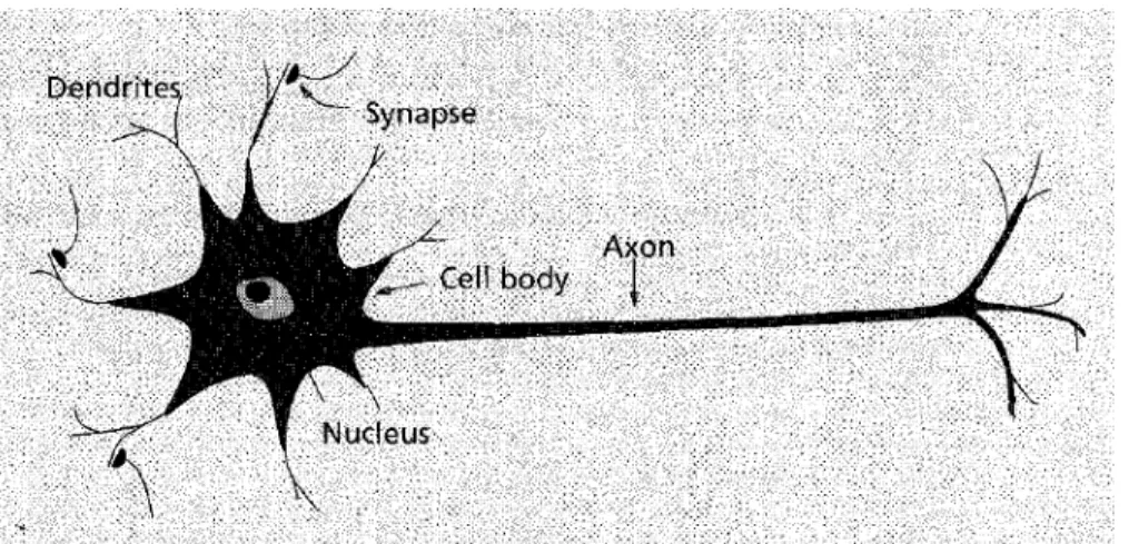
According to the basic definition, ANNs are comprised of a number of extremely linked, adaptive and simple groups of elements that are capable of exceptionally complex and parallel computations for data processing and artificial intelligence (AI) [43]. ANNs are inspired from the actual structures of the biological neurons and their functionality and construction can be seen in the modern computing like AI. The structure of biological neuron is quite simple, having a cell body containing a nucleus that acts as the command center, axons that connects the body part to the synapses and dendrites that act as the transmitters for the neuron. Human brain consists of a large number of such neurons building complexly interconnected nodes. An input is taken by these nodes from the other nodes or the external environment that is then independently processed in the same node causing an activation to produce output that triggers a response to the next layer of nodes or to an external output [44]. Fig. 11 shows the basic structure of the biological neuron [45].

Figure 11: Basic Structure of Biological Neuron

(35)

ANN structure includes three types of layer levels. First is the input layer through which the ANN takes the input, next is the hidden layer where the inputs are actually processed and ANN gives the output through the next in line output layer. The input layer isn’t considered to be a part of the layer structure because it doesn’t perform any computations and hence, have no neurons. Hidden layer level may or may not have multiple number of layers and each hidden layer with multiple neurons. The outputs are specified automatically according to the problem so, the only layer and its number of neurons that are required to be specified is the hidden layer. Fig. 12 specifies the structure of an ANN [46].

Figure 12: Structure of a simple Feed Forward ANN with R inputs, and S number of neurons in hidden layer

The number of layers and neurons in those layers specify the network topology and are important as the classification of ANNs are done on this basis which in turn defines the usage of the network. Due to the complex connections between the nodes and layers, ANN can learn and adapt to a set of sample data and can generalize a vast types of problems. The training of a network and its usage is a relatively easier task, however, selection of a network topology and its parameters is bigger chunk of the work.

4.1.1. Classification of ANNs

ANNs can be classified on the basis of two factors, its usage and the architecture as discussed in [43]. The network architecture consists of the input layer, hidden layer

(36)

including its neurons and output layer together with their transfer or activation functions. A bias is sometimes also added to the total weighed sum of the network layer.

• Architecture

Classification of a network on the basis of its layers’ structure, number of neurons, addition of bias and the connections between the layers comes under the umbrella of its architecture. For simple problems, a simple network with one layer might be enough, but as the problem gets complex, a relatively complex network might be required. A network comprising of more than one layer is known as a multi-layer network and is shown in fig. 13 [46].

Figure 13: A Multi-Layer Feed Forward Network with 3 hidden layers

Further difference in the network can be caused by the backward connections from one layer to the previous ones. A network is called recurrent network if it has a feedback connection from its output to the input of the previous layer and are potentially more powerful than the FFNN [46].

Every layer is connected to the other layer via a weight value and each layers has its own bias value as well. These weights and bias value are updated according to the learning rule that is used to train the network. The functions that define the relationship between the input and outputs of a layer are called transfer functions and any transfer functions from many given functions can be used according to the problem’s requirement. Most commonly used transfer functions are Linear, Hyperbolic Tangent Sigmoid and Log Sigmoid functions.

(37)

• Usability

The other classification factor is the usage of the network. ANNs are used for a vast types of problems including classification, pattern recognition, function fitting, time-series analysis, data reduction, prediction and control etc. Several types of ANN architectures have been proposed in order to solve these problems. Some of them are SOMs, Kohonen network, Hopfield network, back propagation multi-layer perceptron [47].

4.1.2. Network Learning

There are two types of learning, namely Supervised and Unsupervised learning. In unsupervised learning, the network is not presented by a training sequence, instead it is given a dataset and the network clusters the data into different classes. The method in which a learning algorithm is used to adjust network parameters according to the given training set, is called supervised learning. Supervised learning problems are further classified into two categories, regression and classification problems. In classification, the network is used to map the input vector to one of the discrete output values. As the name suggests, it learns to classify that which specific output class the input vector belongs to. However, in regression, the network maps the input vector to a continuous output, meaning it maps the input variables to some continuous function.

Before the network can be used to solve any given problems, it has first to be trained by giving a sample data on which the network adjusts its weights and biases. The training is done by giving the network a training set of the data and a target set. Network learns on the base of the training set and adjusts its parameters so that it can map the training sequence to the given target sequence. Target sequence is the required output we expect from our network after it is given a new set of data to generalize. During the training part, network learning is carried out i.e. network adjusts its parameters according to specific set of rule. These set of rules are defined by different specified Training Algorithms. Different training algorithms are used for different set of problems and for different network architectures. The problem of channel estimation comes under the umbrella of regression, and Resilient Backpropagation (Rprop) algorithm is used as the training function.

(38)

4.2. Multilayer Perceptron (MLP)

In supervised learning standard, network is provided by a required output d for each input pattern. During the learning process, the output y generated by the network may not be equal to the required output d. The difference between these network output and the desired output gives the error i.e. 𝑒𝑒 = 𝑑𝑑 − 𝑦𝑦. The concept of perceptron is to use this error to readjust the layer weights and biases so that this error can be minimized [45]. A network with this error correction rule and having more than one layer, is known as a Multilayer Perceptron (MLP). An MLP is a FFNN with having multiple layers and an error back-propagation rule. The network learning is performed only when the network makes an error [45]. Due to its simplicity and better error correction performance, MLP combines with Rprop algorithm, is our first choice to use as the network architecture for the channel estimation.

4.2.1. MLP Training with Resilient Backpropagation (Rprop)

The resilient backpropagation learning algorithm is a gradient-based batch update setup that works on the basis of Manhattan Update rule. The need of Rprop arises from the fact that the ANNs use sigmoid functions in the layers that work on the basis of slope approaching zero when input gets large. This causes problem when we try to train the ANNs with Steepest Descent algorithm. Rprop solves these issues with the magnitude of the direction and, hence, only takes in account the sign of the derivative.

After the cascade-correlation algorithm and Levenberg-Marquardt (LM) algorithm, Rprop is the fastest weights update algorithm. LM being fast takes more memory and this prohibits to use LM in our case of large network. As we’ll see in the next chapters that the size of the network is directly proportional to the resolution 𝜌𝜌 and the number of subcarriers 𝑁𝑁 used for our communication system model because of sparsity, so the use of Rprop is the best choice as the training algorithm for our network.

4.3. Proposed ANN for Channel Estimation

As discussed in the previous section that the type of network used in this study is the multilayer perceptron with Rprop algorithm as the training function. Further details about the complete ANN models will be discussed in the subsequent sections. The

(39)

simulations, data generation and all other functions being performed are done in Matlab® environment. In this chapter, the name of those variables will be defined and used for notational simplicity.

4.3.1. ANN Model

After the decision about the network type and the training function have been made, the other parameters of the network architecture are to be found and the complete model is then devised using those parameters. The most important steps making use of afore-mentioned parameters are given as follows:

• Generation of sample space o Data preparation

 Training set  Target set

 Ratio of training set to be used as train, validation and test subsets  Normalization of data vectors with zero mean and unit variance • Layers transfer functions

• Find optimal initial values for o Weights’ matrix

o Number of hidden layers

 Number of neurons in each hidden layer • Training and optimization of the network

• Use of the optimized network

After a hit and trial method and training a number of NNs with different initial conditions, several different number of neurons and hidden layers, we select the NN with the best performance. This is further discussed in the following subsection.

Please note that there is no proved way of finding an optimized NN for a specific problem. However, by optimization here we mean to select the best NN on the base of its performance, among several trials with different initial conditions.

(40)

4.3.2. Generation of Sample Space and Preparation of Inputs

Before creating the required neural network, it is important that we have the sample data in the form as required by the input of the network. The input to the network will be a collection of pilot symbols of the received OFDM signals generated by the models as discussed in the previous chapters. The target vectors will be a collection of the known equivalent channel vectors c specific to the received pilots. Each received signal in the training set have a corresponding target set of the channel coefficients specific to its received signal.

For the generation of the training and target dataset, the observation model given in (7) is used. The training set used in our simulations is made up of multiple parts, each part contains multiple samples (i.e. 200) of the received pilot symbols collected for a specific SNR level. Similarly, the next parts of the training dataset are produced for other SNR values and all the parts are collected in one matrix. The SNR values used for the production of training and target datasets are from 𝑆𝑆𝑁𝑁𝑆𝑆 = 11 to 𝑆𝑆𝑁𝑁𝑆𝑆 = 30 with the step of size 3. This completes our training dataset. The target dataset is the collection of the equivalent discrete-time channel vector 𝒉𝒉[𝒏𝒏] specific to the received pilot symbols in the training set. The total number of samples in the sample space of training and target sets are: {# 𝑜𝑜𝑓𝑓 𝑠𝑠𝑎𝑎𝑠𝑠𝑒𝑒𝑙𝑙𝑒𝑒𝑠𝑠 𝑓𝑓𝑜𝑜𝑓𝑓 𝑒𝑒𝑎𝑎𝑐𝑐ℎ 𝑆𝑆𝑁𝑁𝑆𝑆 𝑣𝑣𝑎𝑎𝑙𝑙𝑣𝑣𝑒𝑒 (500) × # 𝑜𝑜𝑓𝑓 𝑆𝑆𝑁𝑁𝑆𝑆 𝑣𝑣𝑎𝑎𝑙𝑙𝑣𝑣𝑒𝑒𝑠𝑠 (7) = 3500}.

Training method plays a vital role in NN performance and the data used for the training impacts the training significantly. This gives basis of the fact that we trained our NN with signals for different SNR levels so that it can learn the impact of SNR on the system; and can use it to effectively predict the channels with differing SNR levels.

(41)

Figure 14: MLP-ANN model used with separate Real and Imaginary Inputs

A fact to keep in mind at this point is that the network does not take arbitrary values as inputs and only takes real valued sample space. Therefore, we separate the samples of sample space into real and imaginary parts. Separating the real and imaginary values of input and target vector and vertically concatenating them into a training and target sequences solves the above hurdle and network now have two inputs with the vector from real values on top and the one from imaginary on the bottom. Let us denote the matrix consisting of the samples space for training and target set as 𝜲𝜲 and 𝜢𝜢 respectively.

The output of the network will also be the same and the real and imaginary parts are then joined at the output by doing the reverse process that was done at the input. Therefore, the model of our network looks like as shown in fig. 14.

The training and target sets are then divided into three subsets with train subset to train the network, validation subset to check the how well network performs on generalization and a test set to test the performance of the network on unseen data. The actual training and target sets are divided, however, the indices of the sample space are made fixed for subsequent subsets. The indices are get by using the dividerand() function of Matlab® by giving it the ratios of the subsets. The indices gotten from this function are then used to update the network parameter related to the index values of the subsets, which will be discussed in the following sections.

(42)

4.3.3. Network Creation and Training

Next step is to create a network with the above given functions and an optimal set of parameter such as initial values of weight and bias matrices, and hidden layers’ matrix 𝑶𝑶. 𝑶𝑶 contains a combination of different number of hidden layers with different number of neurons for each layer. The optimal parameters are obtained by training the network in a nested loop with the outer loop running for each combination of hidden layers 𝑶𝑶 and the number of neurons while the inner loop runs a number of times e.g. 5 for different random initial values, and the performances for each of these combinations stored in a vector. At the end of this nested loop, the performances are compared and the network with the best performance is used in estimation process. The performances of these network architecture are calculated using the Matlab®’s perf() function that calculates MSE for a set of input variable specified to a network. The network with the lowest value is the network with optimal parameters under the current settings.

Figure 15: Performance vector for multiple trainings

Fig. 15 gives an insight to the performance vector when a network is trained five times. It can be seen that each run of the training produced different performance. The network with performance in index 2 was used. As it can be seen in Fig. 16, that the default transfer functions for each layers are used. The transfer function for hidden layers is tansig.

The final network model for training is shown in the following figure:

(43)

Figure 16: Neural Network model after training (nntraintool)

The neural network used for the channel estimation uses one hidden layer with 500 neurons and one output layer. The size of the output layer of the neural network is directly related to the resolution factor 𝜌𝜌 while the number of input connections are dependent upon the pilot spacing Υ. Table 1 shows the final neural network parameters and functions used in training in reference to the model showed in fig. 16.

Table 1: ANN Parameters and Functions

Parameter Value Parameter Value

# of outputs 1 # of inputs 1

# of hidden layers 1 # of hidden

neurons 500

Input size 𝑁𝑁𝑝𝑝× 2 # of samples 4000

# of layers 1 Bias connect [1; 1]

Input connect [1; 0] Layer connect [0 0; 1 0]

Output connect [0 1] Adapt function ‘defaultderiv’

Divide function ‘dividerand’ Divide Parameters [0.5 0.2 0.3]

Performance Func. ‘MSE’ Train function ‘trainrp’

(44)

4.4. Estimated Channel:

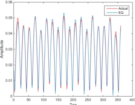
After the network has been trained with the training sequence, it is now ready to be used as a channel estimator. The estimated channel is then equalized and the symbol error rate (SER) is calculated for several values of SNR. Fig. 17 shows the SER-SNR plot for the system using the NN based estimator. The estimator has performed well for the overall system performance and SER is not far from the equivalent channel vector in performance.

Figure 17: Performance comparison for ANN estimate, original and equalized channel (𝜌𝜌=8,

𝛶𝛶=8)

(45)

5. Simulations Results

Simulations for a number of different OFDM parameters, MP algorithm and with different network topologies and architectures were carried out using Matlab®’s simulation environment. A computer with the following specification was used for running the simulations (table 2).

Table 2: PC Resources and Capabilities

Item Value

System Type X64-based PC

Processor Intel core i7-4500U CPU @ 1.81 GHz

Total Physical Memory 16 GB

Total Virtual Memory 25GB

Parallel Computing Capability Yes (NVidia GPU)

Following table shows the parameters used for the communication system under consideration in this study – unless specified otherwise.

Table 3: Communication System's Parameters

Parameter Value

No. of sub-bands (N) 512

No. of used sub-bands (K) 180 * N/256;

Subcarrier spacing (∆𝒇𝒇) – LTE 15*KHz

Bandwidth 10*MHz * N/1024

Carrier frequency (𝒇𝒇𝑨𝑨) 2.5*GHz

Constellation type QPSK

No. of multipath 3

(46)

5.1. Performance Analysis of ANN and MP Algorithms

The performance based comparisons are done in this chapter for both channel estimators discussed in the preceding sections. Monte-Carlo simulations were done on both methods and the comparative figures are drawn from such simulations. We compare the efficiencies in terms of SER and SNR values and the simulation results show the gain and loss in terms of SER. The channel estimators are also compared in terms of the factors that have been discussed in the previous sections that affect the efficiency of the estimators.

Fig. 18 is SER-SNR comparison of original & equivalent channel representations, MP and NN algorithms. It can be seen here that the SER performance of the system using NN estimator is equal to the MP estimator at the SNR of 12dB. The NN performs better at the lower values of SNR than the MP algorithm; where the noise factor in the system is quite large. However, MP algorithm has better performance for the higher values of SNR.

Figure 18: Performance comparison for ANN & MP estimate, original and equalized channel (𝜌𝜌=8, 𝛶𝛶=8)

(47)

These results can further be improved by applying linear MMSE for estimating the pilot symbols; for the received signals that are used for the training of the ANN algorithm. Until this point, the NN was trained with the received pilot symbols as the training set and the actual equivalent channel vector as the target sequence. However, now we show that the LMMSE channel estimator can be used to estimate the channel for the received pilot symbols which in turn become the input of the NN for the training period. This will train the NN in a way that the inputs and the outputs will be closer to each other and will in turn enhance the estimation capability of the NN. The target sequence for ANN training will be kept same as before.

The required information for the application of LMMSE are the Noise power 𝑁𝑁0 and the

correlation matrix 𝑹𝑹 of the channel. With these requirements discussed in above sections, LMMSE can now be applied to the pilot symbols. The input matrix for the input of neural network 𝑿𝑿 is now modified and more refined values are provided to the NN. The improvement in the performance of NN algorithm is considerable and is shown in fig. 19. With the SER improvement, the SNR cutoff point for ANN and MP has also moved from 𝑆𝑆𝑁𝑁𝑆𝑆 = 12 to 𝑆𝑆𝑁𝑁𝑆𝑆 = 14.

Figure 19: Performance comparison for LMMSE-ANN & MP estimate, original and equalized channel (𝜌𝜌 = 𝛶𝛶 = 8) 35

(48)

The above figure forms the major contribution of this work. It can be seen that by using LMMSE, the ANN based channel estimation produce better SER performance of the system.

5.1.1. Effect of 𝜌𝜌 and Υ values

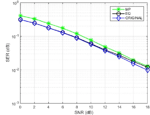
Keeping the updates in the settings mentioned above, the size of pilot spacing Υ and 𝜌𝜌 will also affect the performance of both algorithms. Increasing 𝜌𝜌 to 20 and keeping Υ = 8; we show in fig. 20 that – though the difference is small – the performance for ANN has dropped. NN becomes sensitive to the lower SNR values and now equals to the performance of MP at SNR=10.

Figure 20: Performance comparison for ANN & MP estimate, original and equalized channel (ρ=20, Υ=8) Using the same parameters as in the fig. 20 but with LMMSE, the comparison is shown in fig. 21. If we relate fig. 19 with fig. 21, we see that even with LMMSE, increasing the resolution decreases ANN’s performance slightly. One interesting fact that needs a mention here is that performance of ANNs is quite sensitive to the change in its input in terms of system performance. The reason being, this network architecture was carefully selected after intense simulations and is specific to the problem size and type. However,

(49)

the complexity of the system is not much affected by these changes. On the other hand, the overall performance in terms of SER is improved for all the systems as shown in the following figure.

Figure 21: Performance comparison for LMMSE-ANN & MP estimate, original and equalized channel (ρ=40, Υ=8)

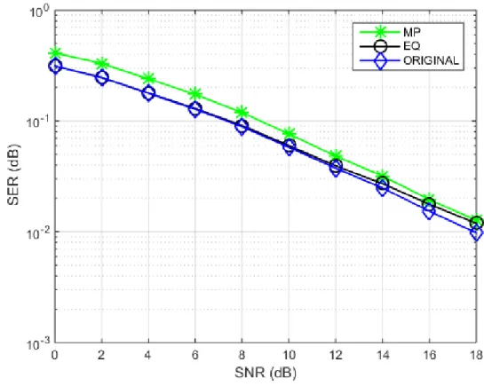
To further the discussion, lets now change 𝜌𝜌 to 16 and Υ to 16; the effect on the performance of both algorithms can be observed in Fig. 22. From fig. 22 it is clear that the pilot spacing cannot be increased from a certain point. This decreases the total number of pilot symbols and the overall efficiency of the system becomes unacceptable. Most acceptable pilot spacing is Υ = 8, after that the system performs poorly regardless the algorithm used for estimation. However, we see that the proposed NN algorithm performs a little better under tougher conditions.

(50)

Figure 22: Performance comparison for ANN & MP estimate, original and equalized channel (ρ=16, Υ=16)

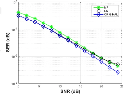
After the SER comparisons of the systems being discussed have been debated above, following figures will compare the mean-squared error (MSE) of these systems. The following fig. 23 is the MSE comparison between the MP and ANN based systems for 𝜌𝜌 = 40 and 𝛶𝛶 = 8. Here we can see that the ANN based systems perform a lot better even in terms of MSE as compared to the MP based systems. ANN based system performs a lot better than MP based system in the presence of smaller SNR values up to the point where 𝑆𝑆𝑁𝑁𝑆𝑆 = 16. The system parameters for this MSE comparison are same as system parameters used in fig. 21. Fig. 23 gives the MSE comparison between MP and ANN based systems for 𝜌𝜌 = 40 and 𝛶𝛶 = 8. It can be observed in the following figures that the cutoff point between the performances of ANN and MP based algorithms is at 𝑆𝑆𝑁𝑁𝑆𝑆 = 14 and this MSE value is better for greater value of 𝜌𝜌 – even though the difference is small.

(51)

Figure 23: MSE vs SNR comparison of MP and ANN based systems (𝜌𝜌 = 40, 𝛶𝛶 = 8)

Figure 24: MSE vs SNR comparison of MP and ANN based systems (𝜌𝜌 = 2, 𝛶𝛶 = 8) 39

(52)

5.2. Complexity Analysis

The channel estimation algorithms can become computationally inefficient as a matrix inversion is required in most of the classical algorithms. The size of this matrix increases with the increased number of inputs and so does the overhead due to the inversion. ANNs, however, do not require any matrix inversion, therefore, are proven to be less complex. Computational complexity is a separate field of study altogether that deals with the classification of computational problems according to their difficulty and relate these complexity classes with each other. In other words, computational complexity theory helps in determining the practical limits on what computers are capable of and what they’re not.

A problem is supposed as difficult if it requires significant resources to be solved no matter what algorithm is used. The theory discusses different problems on the basis of their difficulty by giving models of computations, and measures the resources required to solve these problems – like storage and time. Several classes of complexity are used to classify problems on the basis of above facts and are supposed to have different resource requirements. Non-deterministic Polynomial (NP) is one of the classes of computational complexity with variates as NP-hard and NP-complete. A sparse approximation of a signal is an important issue in many fields today and many algorithms have been proposed for a good sparse approximation in polynomial time like MP. But to design an algorithm that gives a good approximation performance and is flexible in complexity for the large signal dimensions. Also, the universal problem of finding the best m-term estimate is non-deterministic polynomial (NP-Complete) [27].

The computational complexity of algorithm is defined as the number of steps/calculations it has to make in order to solve a problem given an amount of space and time. The space complexity is ignored when comparing the computational complexity of algorithms and time complexity is used. The complexity of an algorithm is often expressed using big O notation.