COMPARISON OF DIFFERENT INTERPOLATION TECHNIQUES IN
DETERMINING OF AGRICULTURAL SOIL INDEX ON LAND
CONSOLIDATION PROJECTS
Mevlut Uyan1
1Selcuk University, Vocational School of Technical Sciences, Konya, Turkey ([email protected]);
ORCID 0000-0002-3415-6893
*Corresponding Author, Received: 10/05/2018, Accepted: 13/06/2018
ABSTRACT: Land consolidation (LC) is a tool to improve the processing efficiency of agricultural area and the promotion of rural development same time an indispensable application for the promotion of sustainable agriculture. In order to achieve the reallocation process after LC, determining the correct of soil index (SI) for each of the agricultural parcels is very important for the success of LC projects. Nowadays, interpolation methods are extensively applied in the mapping processes to estimate the SI at unsampled sites.
The objective of this study was to evaluate and compare the performance of three interpolation methods for the agricultural SI values maps with GIS technology for LC projects. The SI data were determined from 132 observation points. Three spatial interpolation methods Ordinary Kriging (OK), Inverse Distance Weighted (IDW), and Radial Basis Functions (RBFs) were utilized for modeling the agricultural SI values. The results indicated that all methods provided a high prediction accuracy of the mean concentration of SI.In this study, although the best performed interpolation method was the OK, the results showed that the performance differed slightly among three methods. Results show that all the methods present a good performance in the estimation with RMSE (root mean square error) and ME (mean error) close to 0%. Keywords: Land consolidation (LC), Soil index (SI), Ordinary Kriging (OK), Inverse Distance weighting (IDW), Radial
1. INTRODUCTION
Agriculture is the most important and indispensable part of Turkey's economy. The agriculture sector in Turkey still maintains the distinction of being social and economic sector with the effect of nutrition and labor, contribution to GDP and raw materials provided to the industrial sector. The majority of the industrial plant in Turkey use as agricultural raw materials. This situation is of great importance in the development of the industry. Approximately one-third of the population earns one's keep with agricultural activities. Agricultural production has exceeded $ 60 billion for 2015 in Turkey.
Agricultural land fragmentation, in which a single farm uses several parcels of land, is a common phenomenon in many countries (Orea et al., 2015; Latruffe and Piet, 2014). Land fragmentation is the biggest problem for sustainable agriculture (Uyan, 2016). It causes an increase in traveling time between fields which induces both lower labor productivity and higher transport costs for inputs and outputs and reduces the efficiency of machines compared to that obtainable in large, rectangular fields (Orea et al., 2015). In Turkey, the main cause of land fragmentation over the past has been population pressure on agricultural land.
Land consolidation (LC) is one of the most important tools for rural development and avoiding the negative impact of land fragmentation on agricultural productivity (Muchová et al., 2016; Guo et. al., 2015). LC may be described as a planned readjustment and rearrangement of land parcels and their ownership. With LC, land quality and agricultural infrastructures such as irrigation systems and roads are improved, and land fragmentation is reduced (Wang et al., 2015).
In Turkey, LC projects began in 1961. Only 450,000 ha of fragmented agricultural land were consolidated from 1961 to 2002. 5 million ha of fragmented agricultural land were consolidated between 2002 and 2013. The aim is to consolidate 1 million ha of fragmented agricultural land for each year and complete the land consolidation in Turkey until 2023 (Esen et. al., 2017).
Land reallocation stage is the most important step of consolidation. The purpose of this step is to ensure equivalent that the new parcels will be given to the landowners after LC with their previous parcels (Uyan, 2016). Land degrees (valuation) maps are created for this process by valuation experts (Derlich, 2002). Errors in degrees maps cause uneven distributions among landowners. Although soil quality defined as soil index (SI) is not the only factor in valuation, it is the most important factor. The value of a parcel can be affected all factors that have a substantial impact on the use of the agricultural land.
SI based on solely the soil characteristics and is obtained by evaluating factors such as soil depth, structure of the surface layer, subsoil characteristics, drainage, salinity, alkalinity, pH, erosions and relief. Soil index is rated productivity capabilities, potential benefit opportunities according to the land of the soil characteristics. SI is marked as 100 points.
Soil index is calculated according to the following formula:
X
C
B
A
SI
*
*
*
(1)where A is the topsoil profile group (the kind of main material, shape and accumulation formation, age of soil material, variation, erosion resistance), B is the topsoil texture (sand, silt and clay rates according to various size groups in topsoil), C is the land slope and X is the soil profile group (drainage, salinity, alkalinity, acidity, toxicant and erosions (Uyan, 2016).
If SI values cannot be determined reliably for a study area, LC projects is affected negatively. Different interpolation techniques can be used in order to estimate the unmeasured points in accordance with the data values measured in the SI values. Rare measured SI data contain considerable uncertainty. Therefore, mapping the spatial distribution of SI requires spatial interpolation methods. Geographic Information System (GIS) techniques play an important role in managing complex relationships such as the storage, processing, and analysis of a wide variety of spatial data (Kuşçu Şimşek et al., 2018). Surface interpolation methods in a GIS are very powerful tools for predicting surface values. Geostatistics provides very useful techniques for handling spatially distributed data (Mirzaei and Sakizadeh, 2016). Geostatistical interpolation techniques utilize the statistical properties of the measured data to produce the raster maps (Kamali et al., 2015).
The kriging methods are widely applied to geographical sciences as the best linear unbiased prediction technique (Zhu et al., 2016; Peng et al., 2014). Likewise, the inverse distance weighting (IDW) interpolation algorithm is also one of the most commonly used spatial interpolation methods in geographical sciences (Mei and Tian, 2016). The most frequent applications for establishing spatial representations rely on the principle of ordinary kriging (OK) or IDW (de Amorim et al., 2016). Radial Basis Functions (RBFs) is known as a powerful tool for scattered data interpolation problem (Su et al., 2015) and widely applied to approximate scattered data (Zhang and Li, 2016).
The purpose of this study was to evaluate and compare the performance of three interpolation methods (Ordinary Kriging (OK), Inverse Distance Weighted (IDW), and Radial Basis Functions (RBF)) for the agricultural SI values maps with GIS technology for LC project in the village of Ortaoba in the Karaman Province, Turkey.
2. MATERIAL AND METHODS 2.1 Study Area
Ortaoba Village covers an area of approximately 2700 ha in the Karaman Province, Turkey. It is located 42 km away in the northwest of Karaman (Fig. 1). The topographical structure is generally flat and close to flat. The cultivated products are mostly wheat, barley and chickpea. The SI data were determined from 132 observation points.
Documents of cadastral parcels, SI data and other information on the area were obtained from the Konya Provincial Directorate of Agriculture.
Figure.1 Study area and spatial distribution of sample points
2.2 Interpolation methods
2.2.1 Ordinary kriging (OK)
The OK method is widely applied to geographical sciences as the best linear unbiased prediction technique because it minimizes the variance of estimation error based on the statistical properties of the random field. The accuracy of OK is highly dependent on the effectiveness of the stochastic model of the random field (Zhong et al., 2016; Zhu et al., 2016). OK uses a linear combination of weights at known points to estimate the value at an unknown point (Uyan, 2016). OK assumes a constant, but unknown, local mean of a random variable, which is not plausible when spatial data exhibit a strong trend (Cafarelli et al., 2015). The OK method was detailed at Uyan (2016).
The general equation of the kriging method is as follows (Uyan, 2016):
∗ = ∑ ( ) (2)
In order to achieve equitable estimations in ordinary kriging the following set of equations should be solved simultaneously.
)
,
(
)
,
(
1 j i j i n i i
x
x
x
x
(3)1
1
n i i
(4)Here, Z*(xp) is the kriged value at location xp, Z(xi)
is the known value at location xi, λi is the weight
associated with the data, µ is the Lagrange multiplier, and γ(xi, xj) is the value of variogram corresponding to a
vector with origin in xiand extremity in xj.
2.2.2 Inverse distance weighted (IDW)
A type of deterministic method widely applied in spatial modelling (de Amorim et al., 2016). The IDW calculates the interpolated values of unknown points by
weighting average of the values of known points. The name given to this type of methods was motivated by the weighted average applied since it resorts to the inverse of the distance to each known point when calculating the weights (Mei and Tian, 2016). The IDW interpolation method is mathematically expressed as (Osmanli et al., 2017):
N i n i N i n i i d d z Z 1 1 0 . (5) where:Z0=The estimation value of variable z in point I.
Zi= The sample value in point I.
di= The distance of sample point to estimated point.
N= The coefficient that determines weigh based on a distance.
n= The total number of predictions for each validation case.
2.2.3 Radial basis functions (RBFs)
RBFs method is one of the primary tools for interpolating multidimensional scattered data and used a basic equation dependent on the distance between the interpolated point and the sampling points for calculating smooth surfaces from a large number of data points (Xie et al., 2011). RBFs have become a popular numerical technology for scattered data approximation in a wide variety of fields for solving partial differential equations (Boyd, 2015). The prediction value by RBFs can be expressed as the sum of two components (Xie et al., 2011):
( ) = ∑ ( ) + ∑ (6)
where ψ(dj) shows the radial basis functions and djthe
distance from sample site to prediction point x, fi(x) is a
trend function, a member of a basis for the space of polynomials of degree <m. The coefficients aiand bjare
calculated by means of the resolution of the following system of n+m linear equations; n is the total number of known points used in the interpolation as below:
( ) = ∑ ( ) + ∑ = 1,2, … (7)
∑ = 0 = 1,2,3, … (8)
RBFs methods have five different basis functions (thin plate splines, spline with tension, completely regularized spline, multiquadratic function and inverse multiquadratic function). We used thin plate splines
(TPS) function in this study because it gave the lowest estimation error. The basic equation for TPS is below (Xie et al., 2011):
( ) = ln (9)
where d is the distance from sample to prediction location, c is a smoothing factor.
2.3 Comparison of interpolation methods
Cross validation and validation with an independent data set are the commonly used methods for comparing the interpolation methods (Xie et al., 2011). Cross validation is an estimator widely used to estimate generalization error for its practicability and flexibility (Jiang and Wang, 2017). Cross-validation was obtained by taking the value of a sample point out and estimating it from the remaining values. The errors produced (observed-predicted) were used to assess the accuracy of each interpolation method. In order to assess the performance of different interpolation methods, the mean error (ME) and the root mean square error (RMSE) were calculated according to the formulas (Pereira et al., 2015):
= ∑ { ( ) − ̂ ( )} (10)
= ∑ { ( ) − ̂ ( )} (11)
Where
( )
is the observed value,̂( )
predicted value and N the number of data points. Lower ME and RMSE values indicate fewer errors. If these values are small enough, interpolation becomes so accurate. Cross validation only confirms the prediction accuracy at sampling sites and cannot reflect the accuracy at unsampled sites (Cui et al., 2016).In this study, all of the digitization, conversion and analysis processes of the maps were performed using ArcGIS 9.3 software.
3. RESULTS AND DISCUSSION
The descriptive statistics of SI parameters have been given in Table 1. According to this table, the calculated SI ranged from 10.53 to 100 with a mean value of 46.14. The interpolation methods give the best results if the distribution of samples to be normal distributed. Otherwise, a suitable log transformation should be applied to the sample data. According to Table 1 results, histogram of SI values was plotted with a normal distribution curve.
Considering OK method, the nugget-sill rate can be used to classify spatial dependency. If the result is <25, 25–75, and >75 % suggest intense, medium, and weak spatial autocorrelations, respectively (Mirzaei and Sakizadeh, 2016; Uyan, 2016). The nugget-sill ratio of SI
in the area was 0.23 (23 %), which showed intense spatial autocorrelations according to Table 2.
Table 1 Descriptive statistics of the SI data Statistics SI data Count 132 Minimum 10.53 Maximum 100 Mean 46.14 Std. Dev. 19.94 Skewness 0.48 Kurtosis 2.84 1st Quartile 29.92 Median 44.46 3rd Quartile 57.06
Geostatistical analysis uses the semivariogram to quantify the spatial variation of a regionalized variable and derives important parameters used for kriging spatial interpolation (Reza et al., 2016). Different semivariogram functions (Circular, Spherical, Tetraspherical, Pentaspherical, Exponential, Gaussian) were evaluated to select the best fit with the data. OK validity of semivariogram was assessed using cross-validation parameter Root Mean Square Standardized (RMSS). The estimations for a good-fitting semivariogram are an RMSS near 1. If RMSS < 1, there is a tendency toward overestimation of the variance; if > 1, there is a tendency toward underestimation (Uyan, 2016). Table 2 shows cross-validation indicators of SI obtained from OK method. According to the cross validation parameters, circular model was fitted to the empirical semivariograms. RMSS of circular model is close to 1, more than others. The model fitted to experimental variogram was circular as it results from cross-validation.
Table 2 Cross-validation performance and ranking of OK interpolation method
According to IDW method, ME and RMSE are 1.49, 12.38, respectively.
Five different basis functions (thin plate splines, spline with tension, completely regularized spline, multiquadratic function and inverse multiquadratic function) were evaluated for the RBFs. The accuracy performances of these functions are given in Table 3. Best results were obtained with thin plate splines function.
Table 3 Performance values of RBFs basis functions
ME RMSE Regression
Function Completely regularized spline 0.49 11.62 0.69x+13.6 Spline with tension 0.45 11.64 0.69x+13.7 Multiquadratic function 0.47 11.83 0.75x+10.6 Inverse multiquadratic functio 0.63 11.70 0.68x+13.9
Thin plate splines 0.45 11.62 0.77x+8.99
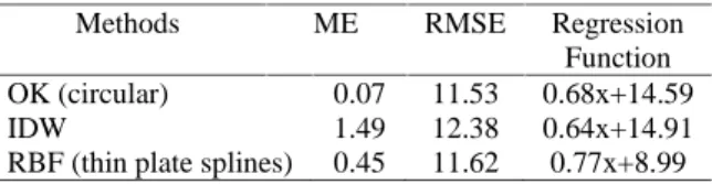
All of the interpolation methods have similar prediction accuracy. Table 4 shows cross-validation indicators of SI obtained from OK, IDW, and RBF methods. The best performance was obtained by OK
(RMSE=11.53). RBF (RMSE=11.62) and IDW (RMSE=12.38) methods performs nearly as well as OK.. The results of three different interpolation methods had a quite similar SI distribution tendency according to Fig. 2.
Table 4
Cross-validation performance and ranking of different interpolation methods for SI
Methods ME RMSE Regression
Function OK (circular) 0.07 11.53 0.68x+14.59
IDW 1.49 12.38 0.64x+14.91
RBF (thin plate splines) 0.45 11.62 0.77x+8.99 The ME shows that bias is very small for three methods. However, the OK method is much better than the others with a value of 0.07. The best fitted regression line between measured and estimated SI values and 1:1 line is showed for OK, IDW and RBF in Fig. 3. The deviation from the 1:1 line is greater for the IDW and OK methods. It shows that within interpolation methods used, the RBF method is the one that best estimated the measurements results of the SI.
If we take the results as a whole, the OK and RBF methods gives better results than the IDW method. ME RMSE RMSS Nugget/sill Regression Function
Circular 0.07 11.53 0.89 0.23 0.68x+14.59 Spherical 0.12 11.89 0.84 0.25 0.68x+14.33 Tetraspherical 0.13 11.89 0.83 0.26 0.68x+14.21 Pentaspherical 0.13 11.89 0.80 0.26 0.68x+14.14 Exponential 0.38 11.74 0.82 0.02 0.69x+13.48 Gaussian 0.09 12.33 0.89 0.49 0.68x+14.94
Figure.2 Interpolation effect of SI in study area through the three interpolation models
Figure.3 Least-squares regression line and the 1:1 line between the measured and the estimated SI values 4. CONCLUSION
Spatially continuous data is often required for environmental sciences and management. However, information for environmental variables is usually collected by point sampling. Thus, methods that generate such spatially continuous data by using point samples become essential tools. Spatial interpolation methods are, however, often data-specific or even variable-specific. Many factors affect the predictive performance of the methods. Hence it is difficult to select an appropriate method for a given dataset (Li and Heap, 2014). Even with the same type of interpolation method, the results varied with the parameters of the method. The target of the interpolations was to estimate the spatial means as accurately as possible (Xie et al., 2011).
Effectiveness of land consolidation depends on accurate and efficient mapping of SI. Usually, a larger number of soil samples will produce a more accurate SI
map. However, due to the cost of sample collection and analysis, the use of large numbers of soil samples is usually impractical.
In this study, according to the RMSE for cross validation, OK and RBF are more accurate than IDW method. IDW have the biggest estimated error. According to Fig.2, SI estimated by OK and RBF gave quite similar results.
Kriging is an example of a group of geostatistical techniques used to interpolate the value of a random field. Kriging is based on statistical models involving autocorrelation. Autocorrelation refers to the statistical relationships between measured points. Not only do geostatistical methods have the capability of producing a prediction surface, but they can also provide some measures of the certainty and accuracy of the predictions (Ly et al., 2013). Kriging gives the best linear unbiased prediction of the intermediate values (Uyan, 2016). In IDW, each interpolated value is a weighted combination of every examination data point. In the classical formulation (IDW), the weights are inversely proportional to power of the distances to the data points (Smith et al., 2017). RBF methods are a series of exact interpolation techniques; that is, the surface must pass through each measured sample value (Liu et al., 2016).
SI values of land are one of the important criteria for LC studies. Therefore, it must be determined very precisely (Uyan, 2016). This study is conducted by making spatial analyses of 132 observation points using interpolation methods in order to determine the agricultural SI values in the LC project area. Tested three interpolation methods have a high prediction accuracy of the mean content for SI. The best performance was obtained by OK (RMSE=11.53). RBF (RMSE=11.62) and IDW (RMSE=12.38) methods performs nearly as well as OK. The results of three different interpolation methods had a quite similar SI distribution tendency according to Fig. 2. The best fitted regression line between measured and estimated SI values and 1:1 line was determined by RBF (y=0.77x+8.99). The modeling results show that the interpolated SI values similarly matched the observed SI values.
REFERENCES
Boyd, J.P. (2015). Convergence and error theorems for Hermite function pseudo-RBFs: Interpolation on a finite interval by Gaussian-localized polynomials, Applied Numerical Mathematics 87, 125-144.
Cafarelli, B., Castrignan, A., De Benedetto, D., Palumbo, A.D., Buttafuoco, G. (2015). A linear mixed effect (LME) model for soil water content estimation based on geophysical sensing: a comparison of an LME model and kriging with external drift, Environmental Earth Sciences 73(5), 1951-1960.
Cui, Y. Q., Yoneda, M., Shimada, Y., Matsui, Y. (2016). Cost-Effective Strategy for the Investigation and Remediation of Polluted Soil Using Geostatistics and a Genetic Algorithm Approach, Journal of Environmental Protection 7(01), 99-115.
de Amorim Borges, P., Franke, J., da Anunciação, Y. M. T., Weiss, H., Bernhofer, C. (2016). Comparison of spatial interpolation methods for the estimation of
precipitation distribution in Distrito Federal, Brazil, Theoretical and applied climatology 123(1-2), 335-348. Derlich, F. (2002). Land Consolidation: A Key for Sustainable Development – French Experience, FIG XXII International Congress, Washington, USA. Esen, Ö., Çay, T., Toklu, N. (2017). Evaluation of Land Reform Policies in Turkey, International Journal of Engineering and Geosciences 2(2), 61-67.
Guo, B., Jin, X., Yang, X., Guan, X., Lin, Y., Zhou, Y. (2015). Determining the effects of land consolidation on the multifunctionlity of the cropland production system in China using a SPA-fuzzy assessment model, European Journal of Agronomy 63, 12–26.
Jiang, G., Wang, W. (2017). Markov cross-validation for time series model evaluations, Information Sciences 375, 219-233.
Kamali, M. I., Nazari, R., Faridhosseini, A., Ansari, H., Eslamian, S. (2015). The Determination of Reference Evapotranspiration for Spatial Distribution Mapping Using Geostatistics, Water Resources Management 29(11), 3929-3940.
Kuşçu Şimşek, Ç., Türk, T., Ödül, H., Çelik, M.N. (2018). Detection of Paragliding Fields by GIS, International Journal of Engineering and Geosciences 3(3), 119-125.
Latruffe, L., Piet, L. (2014). Does land fragmentation affect farm performance? A case study from Brittany, France, Agricultural Systems 129, 68–80.
Li, J., Heap, A.D. (2014). Spatial interpolation methods applied in the environmental sciences: A review, Environmental Modelling & Software 53, 173-189. Liu, Y., Hu, S., Sheng, D., Chang, L., Jia, M. (2016). Study of precipitation interpolation at Xiangjiang River Basin based on Geostatistical Analyst, In Geoinformatics, 2016 24th International Conference on (pp. 1-5). IEEE.
Ly, S., Charles, C., Degré, A. (2013). Different methods for spatial interpolation of rainfall data for operational hydrology and hydrological modeling at watershed scale. A review, Biotechnologie, Agronomie, Société et Environnement 17(2), 392.
Mei, G., Tian, H. (2016). Impact of data layouts on the efficiency of GPU-accelerated IDW interpolation, SpringerPlus 5(1), 104.
Mirzaei, R., Sakizadeh, M. (2016). Comparison of interpolation methods for the estimation of groundwater contamination in Andimeshk-Shush Plain, Southwest of Iran, Environmental Science and Pollution Research 23(3), 2758-2769.
Muchová, Z., Leitmanová, M., Petrovič, F. (2016). Possibilities of optimal land use as a consequence of lessons learned from land consolidation projects (Slovakia), Ecological Engineering 90, 294-306.
Orea, L., Perez, J. A., Roibas, D. (2015). Evaluating the double effect of land fragmentation on technology choice and dairy farm productivity: A latent class model approach, Land Use Policy 45, 189-198.
Osmanli, N., Sert, E., Uyan, M. (2017). Social texture map and Social Information Center design and integration for social welfare in the city of Konya, Turkey, International Social Work 60(2), 521-533. Peng, X., Wang, K., Li, Q. (2014). A new power mapping method based on ordinary kriging and determination of optimal detector location strategy, Annals of Nuclear Energy 68, 118-123.
Pereira, P., Oliva, M., Misiune, I. (2015). Spatial interpolation of precipitation indexes in Sierra Nevada (Spain): comparing the performance of some interpolation methods, Theoretical and Applied Climatology 126(3), 1-16.
Reza, S. K., Baruah, U., Sarkar, D., Singh, S. K. (2016). Spatial variability of soil properties using geostatistical method: a case study of lower Brahmaputra plains, India. Arabian Journal of Geosciences, 9(6), 1-8.
Smith, T.B., Smith, N., Weleber, R.G. (2017). Comparison of nonparametric methods for static visual field interpolation, Medical & biological engineering & computing 55(1), 117-126.
Su, L.D., Jiang, Z.W., Jiang, T.S. (2015). Numerical Method for One-Dimensional Convection-diffusion EquationUsing Radical Basis Functions. Journal of Physical Mathematics 6(2), 2015.
Uyan, M. (2016). Determination of agricultural soil index using geostatistical analysis and GIS on land consolidation projects: A case study in Konya/Turkey, Computers and Electronics in Agriculture 123, 402-409. Wang, J., Yan, S., Guo, Y., Li, J., Sun, G. (2015). The effects of land consolidation on the ecological connectivity based on ecosystem service value: A case study of Da’an land consolidation project in Jilin province, Journal of Geographical Sciences 25(5), 603-616.
Xie, Y., Chen, T.B., Lei, M., Yang, J., Guo, Q.J., Song, B., Zhou, X.Y. (2011). Spatial distribution of soil heavy metal pollution estimated by different interpolation methods: accuracy and uncertainty analysis. Chemosphere, 82(3), 468-476.
Zhang, Y.F., Li, C.J. (2016). A Gaussian RBFs method with regularization for the numerical solution of inverse heat conduction problems. Inverse Problems in Science and Engineering 24(9), 1606-1646.
Zhong, X., Kealy, A., Duckham, M. (2016). Stream Kriging: Incremental and recursive ordinary Kriging over spatiotemporal data streams, Computers & Geosciences 90, 134-143.
Zhu, Z., Chen, Z., Chen, X., He, P. (2016). Approach for evaluating inundation risks in urban drainage systems, Science of the Total Environment 553, 1-12.