Can Fahrettin Koyuncu1, Salim Arslan1, Irem Durmaz2, Rengul Cetin-Atalay2, Cigdem Gunduz-Demir1*
1 Department of Computer Engineering, Bilkent University, Ankara, Turkey, 2 Department of Molecular Biology and Genetics, Bilkent University, Ankara, Turkey
Abstract
Automated cell imaging systems facilitate fast and reliable analysis of biological events at the cellular level. In these systems, the first step is usually cell segmentation that greatly affects the success of the subsequent system steps. On the other hand, similar to other image segmentation problems, cell segmentation is an ill-posed problem that typically necessitates the use of domain-specific knowledge to obtain successful segmentations even by human subjects. The approaches that can incorporate this knowledge into their segmentation algorithms have potential to greatly improve segmentation results. In this work, we propose a new approach for the effective segmentation of live cells from phase contrast microscopy. This approach introduces a new set of ‘‘smart markers’’ for a marker-controlled watershed algorithm, for which the identification of its markers is critical. The proposed approach relies on using domain-specific knowledge, in the form of visual characteristics of the cells, to define the markers. We evaluate our approach on a total of 1,954 cells. The experimental results demonstrate that this approach, which uses the proposed definition of smart markers, is quite effective in identifying better markers compared to its counterparts. This will, in turn, be effective in improving the segmentation performance of a marker-controlled watershed algorithm.
Citation: Koyuncu CF, Arslan S, Durmaz I, Cetin-Atalay R, Gunduz-Demir C (2012) Smart Markers for Watershed-Based Cell Segmentation. PLoS ONE 7(11): e48664. doi:10.1371/journal.pone.0048664
Editor: Konradin Metze, University of Campinas, Brazil
Received May 15, 2012; Accepted September 27, 2012; Published November 12, 2012
Copyright: ß 2012 Koyuncu et al. This is an open-access article distributed under the terms of the Creative Commons Attribution License, which permits unrestricted use, distribution, and reproduction in any medium, provided the original author and source are credited.
Funding: This work was supported by the Scientific and Technological Research Council of Turkey under the project number TUBITAK 109E206. http://www. tubitak.gov.tr. The funders had no role in study design, data collection and analysis, decision to publish, or preparation of the manuscript.
Competing Interests: The authors have declared that no competing interests exist. * E-mail: [email protected]
Introduction
Automated imaging systems are becoming popular to analyze cellular events of fixed or live cells. These cellular imaging systems have potential not only for decreasing processing time but also for reducing human errors in the analysis. In almost all of the systems, cell segmentation constitutes the first step, which greatly affects the performance of the other system steps. Although there are several algorithms for the segmentation of fixed cell images from a light or a fluorescence microscope, there exist only few for the segmen-tation of live cells from phase contrast microscopy. In this paper, we focus on the implementation of a robust segmentation algorithm for live cells in culture media.
In general, previous studies have approached the cell segmen-tation problem in two different contexts: segmenting monolayer isolated cells and segmenting cells that grow in clumps on layers. For monolayer isolated cell segmentation, the studies first differentiate cell pixels from the background using global thresh-olding [1], adaptive threshthresh-olding [2–5], and clustering algorithms [6] and then consider the connected components of the cell pixels as the segmented cells.
For the segmentation of clumped cells, the previous studies mainly use active contour models and marker-controlled water-shed algorithms. The active contour models define an energy function usually on the edge map of an image, associated with the cell contours, and achieve segmentation by finding the contours that minimize the energy function [7–9]. The marker-controlled watershed algorithms identify the markers, each of which corresponds to a cell, and start the flooding process from these markers. One common way to identify the markers is to find regional minima on the intensity/gradient map of the image,
reflecting the intensity differences between inside and outside of the cells [10–12], and/or on the distance transform of an initially segmented image, reflecting the shape characteristics of the cells [13–16]. There are also other methods that are applied on the transforms to find the markers based on the shape characteristics. These methods include applying iterative erosions [17] and modeling by the mixture of Gaussians [18]. As the marker-controlled watersheds typically cause oversegmentation, the studies commonly perform a merge process on the segmented cells after their watershed algorithms [19–22].
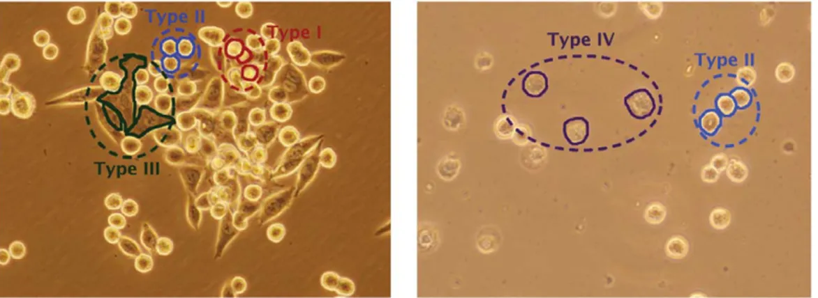
Image segmentation in general is an ill-posed problem. The success highly depends on the intent of segmentation as well as the knowledge about the image content. This is especially the case for the problems, in which domain specific knowledge is necessary even for human subjects to achieve successful segmentations. Live cell segmentation is one of such problems. In live cell images, cells of the same cell line or the same tissue may show different morphologies and intensity/texture characteristics. Moreover, these characteristics could be different from a cell line or a tissue to another. For example, KATO-3 gastric cancer cells can be grouped into four morphological classes based on their visual characteristics (Figure 1). The first group corresponds to round cells with relatively brighter inner and boundary pixels. The second one corresponds to round cells as well but these cells consist of relatively darker pixels in their centers and brighter pixels on their boundaries. The third group corresponds to non-circular cells that have relatively larger and irregular shapes and consist of high-gradient dark pixels. These cells also have brighter pixels on their boundaries. The last group corresponds to apoptotic cells whose inner regions and boundaries turn into matte and irregular.
The algorithms with the capacity of incorporating this kind of biological knowledge into segmentation have potential to improve the results. This is our main motivation behind using domain specific knowledge, in the form of visual characteristics of the cells, in our segmentation algorithm.
In this paper, we propose a new algorithm for the effective and robust segmentation of live cells. In the proposed algorithm, our main contribution is the incorporation of domain specific knowledge into the definition of a new set of ‘‘smart markers’’
for a watershed algorithm. In order to determine the smart markers, the proposed algorithm identifies different pixel groups with different visual properties, based on the biological back-ground knowledge, and processes these groups with respect to each other, again using the background knowledge of different cell characteristics. Working with live cell images taken from the KATO-3 cell line, our experiments demonstrate that the proposed algorithm, which uses this new smart marker definition, is effective in finding better markers compared to its counterparts, which will
Figure 1. Example images of live KATO-3 gastric carcinoma cells. As shown in the images, these cells can be grouped into four morphological classes based on their visual characteristics. Examples from these groups are also indicated on the images.
doi:10.1371/journal.pone.0048664.g001
Figure 2. Schematic overview of the proposed algorithm. doi:10.1371/journal.pone.0048664.g002
in turn improve the segmentation performance of a marker-controlled watershed algorithm. (One should note that the marker term used in this paper is completely different than the one used in immunocytochemistry. Here a marker refers to an image location from which the flooding process of a watershed algorithm starts. The smart marker term is used to indicate that the markers are identified more wisely, considering the visual properties of cells in a cell line.)
The proposed algorithm differs from the previous ones in two main aspects. First, it defines the smart markers based on the background knowledge specific to the image whereas the previous algorithms define them using intensity, gradient, and distance measures without considering the image specific properties. Second, the previous algorithms typically find more markers than the actual cells, resulting in oversegmentation, and hence, they usually necessitate using a merge process after their watershed algorithms. In contrary, the proposed algorithm can find more markers that are one-to-one mapped to the actual cells and can give less oversegmented results without using an external merge process.
Materials and Methods Cell lines
Five different cell lines are used in the experiments. The human gastric cancer cell line (KATO-3) was inoculated in growth medium containing High glucose (4500 mg/L D-Glucose) DMEM with 10% FBS, 1% NEAA, 1% Penicilin/Streptomycin, and 1% L-glutamine. The human liver cancer cell line (Huh7) and the human breast cancer cell line (MCF7) were inoculated in complete growth medium composed of DMEM, with 10% FBS, 1% NEAA and 1% Penicilin/Streptomycin. The human endo-metrial carcinoma cell line (MFE-296) was cultivated in growth medium containing 40% RPMI 1640, 40% MEM (with Earle
salts), 10% FBS, 2 mM L-glutamine and 1| insulin-transferrin-sodium selenite. The human breast cancer cell line (SK-BR-3) was inoculated in complete growth medium composed of HyClone MCCOY’S 5A, together with 10% FBS and 1% L-glutamine. All cell lines were incubated in 370C, 5% CO2, 95% air containing
incubators.
Smart markers algorithm
The proposed algorithm relies on defining three basic types on image pixels—according to the intensity and gradient of these pixels and their surroundings, associating these basic types with the cells of different characteristics, and extracting the markers on each of these basic types by considering the morphological characteristics of their associated cells. The details of this algorithm are explained in the following subsections. A schematic overview of the algorithm is provided in Figure 2.
In this work, we develop our algorithm focusing on the KATO-3 human gastric cancer cell line. Therefore, we consider the characteristics of its cells in the definition of the basic pixel types and the markers. Nevertheless, this idea can also be applied to other cell lines or tissues, provided that the basic types reflecting the characteristics of their cells are defined. In our experiments, we also obtain preliminary results on four different cell lines to explore the applicability of this algorithm to others.
Cell pixel quantization. This part consists of transforming an image into three basic types of pixel groups, each of which corresponds to a cell region of different characteristics. These types correspond to (i) bright pixels, (ii) dark pixels fully surrounded by bright pixels, and (iii) dark pixels only partially surrounded by bright pixels. They are herein referred to as bright, dark-center, and dark pixels, respectively. These three pixel types are used for characterizing the four morphological classes of the KATO-3 gastric cancer cells; these classes are explained in the introduction and illustrated in Figure 1. Particularly, we employ bright pixels
Figure 3. Illustration of the cell pixel quantization step on two exemplary images. (A) Start with an original image, (B) identify bright and dark pixels using the intensity and gradient information, (C) identify some of dark pixels as dark-center pixels, and (D) eliminate noise and artifacts. In this illustration, bright, dark, and dark-center pixels are shown with red, blue, and green, respectively.
doi:10.1371/journal.pone.0048664.g003
Figure 4. Illustration of the iterative erosion algorithm ondark
pixels. (A) before and (B) after. doi:10.1371/journal.pone.0048664.g004
Figure 5. Illustration of the iterative erosion algorithm on dark-centerpixels. (A) before and (B) after.
for characterizing Type I cells as well as the boundaries of the others, dark-center pixels for Type II cells, and dark pixels for both Type III and Type IV cells.
Cell pixel quantization starts with identifying bright and dark cell pixels. Bright pixels correspond to high intensity regions in the image. Hence, we obtain them by thresholding the gray-level image with the Otsu method [23], which automatically computes the threshold tgray on intensity values. Dark pixels correspond to
relatively darker regions with high gradient values. Here one should note that dark cell regions have an intensity distribution similar to the background. Thus, using only intensities, without considering gradient values, would yield errors in pixel quantiza-tion. In this work, we use the Sobel operators on gray-level intensities to define gradient values. Computing a new Otsu threshold tsobel on these gradients, dark pixels are defined as the
pixels whose gray-level intensities are less than tgray and whose
gradients are greater than k:tsobel. Here the Sobel threshold is
multiplied by a constant k since our experiments reveal that relatively lower gradients should also be considered in the dark pixel definition.
After this quantization, dark pixels are further grouped into two based on whether they are fully surrounded by bright pixels; that is, some of the dark pixels are identified as dark-center pixels. However, there usually exists noise in the quantized pixels, which leads to errors in the definition of dark-center pixels. Thus, we postprocess the quantized pixels to alleviate the noise. For that, we first eliminate narrow dark pixel regions around the boundaries of bright regions and then apply a majority filter on the quantized pixels. For the example live cell images shown in Figure 3A, the quantized pixels obtained by this process are illustrated in Figure 3B. In this figure, bright and dark pixels are shown in red and blue, respectively. After this noise elimination, we identify the dark-center pixel group as follows: We consider all pixels except the bright ones and find the connected components on these pixels. Let Cibe the ith connected component and diand bibe the
numbers of dark and background pixels in the component Ci,
respectively. Dark pixels in Ciare identified as dark-center pixels if
diwbi. Otherwise, they remain as dark pixels. Figure 3C illustrates the quantized pixels obtained at the end of this step. Here dark-center pixels are shown in green.
The final step is to eliminate holes and artifacts from the pixel groups. First, we fill holes in between cell pixels provided that the holes are smaller than an area threshold Tarea. In our experiments,
we observe that the main source of noise and artifacts is the dark components. They may correspond to small noisy regions as well as relatively larger artifacts usually found in the background (see the second row of Figure 3). These larger artifacts typically do not contain any bright pixels on their boundaries. Thus, using these observations, we define two rules: First, we eliminate the dark components if they are smaller than the area threshold Tarea.
Second, we eliminate the dark components that do not contain any bright pixels on their boundaries. The quantized pixels obtained at the end of these elimination procedures are shown in Figure 3D. We use these quantized pixels to define our smart markers.
Smart marker extraction. The proposed algorithm defines the markers for each of the three pixel types separately, according to the characteristics of the regions that each type corresponds to. Since the markers are defined considering the background knowledge of the corresponding region characteristics, it is expected to find more markers that are one-to-one mapped to the actual cells, and thus, to obtain less under and oversegmented results.
In order to define the markers on dark and dark-center pixels, we employ an iterative erosion algorithm. This algorithm erodes the given pixel groups iteratively until the size of a group falls below a threshold. In our work, we select this threshold separately for dark and dark-center pixels, considering their region charac-teristics. Since dark-center pixels usually correspond to relatively smaller regions compared to dark pixels, we use a size threshold Tsize for dark pixels and the half of it (Tsize=2) for dark-center
pixels. Similarly, we use a disk structuring element with a radius of rdiskfor the erosion of dark pixels and its half (rdisk=2) for that of
dark-center pixels. The iterative erosion algorithm on dark and dark-center pixels is illustrated in Figures 4 and 5, respectively.
To define the markers on bright pixels, we take the following observation into consideration. Bright pixels can be found both inside a particular class of cells and the boundaries of the others. To alleviate the negative effects of the boundaries, we first dilate the previously found markers and then locate circles on the remaining bright pixels using the modified version of the circle-fit algorithm [24]. In this algorithm, starting from the largest one, we iteratively locate circles on the given pixels provided that the size of a circle is larger than the threshold Tsize and the circle
boundaries are close enough to the non-bright pixels. This circle-fit algorithm on bright pixels is illustrated in Figure 6.
Figure 6. Illustration of the circle-fit algorithm on the bright
pixels. (A) before and (B) after. doi:10.1371/journal.pone.0048664.g006
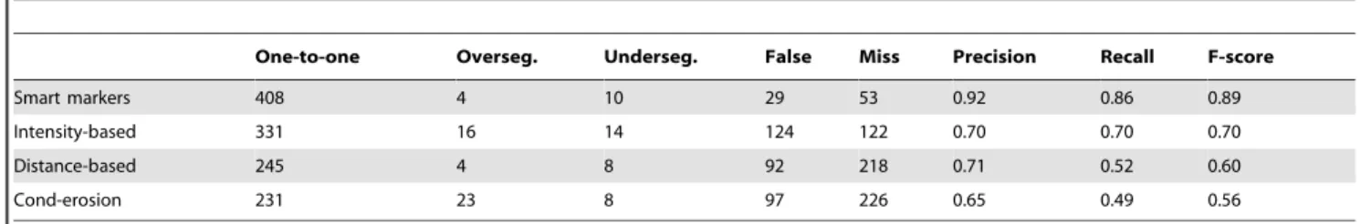
Table 1. Comparison of the proposed smart markers algorithm against different marker identification algorithms.
One-to-one Overseg. Underseg. False Miss Precision Recall F-score
Smart markers 408 4 10 29 53 0.92 0.86 0.89
Intensity-based 331 16 14 124 122 0.70 0.70 0.70
Distance-based 245 4 8 92 218 0.71 0.52 0.60
Cond-erosion 231 23 8 97 226 0.65 0.49 0.56
The results are obtained on the training set using marker-based evaluation. doi:10.1371/journal.pone.0048664.t001
Results Dataset
We conduct our experiments on 44 live cell images of the KATO-3 human gastric cancer cell line. The dataset contains a total of 1954 cells most of which grow in clumps on layers. Each image has a resolution of 1360|1024 pixels. The images are captured by a digital (Olympus DP72, Tokyo, Japan) microscope with a 40| objective lens. The cells are annotated by our biologist collaborators, manually drawing their boundaries. We will use the centroids of these annotated cells for marker-based evaluation and their boundaries for area-based evaluation.
In our experiments, the images are randomly divided into training and test sets. The training set includes 474 cells of 10 different images whereas the test set includes 1480 cells of the remaining 34 images. The cells in the training set are used to estimate the parameters of our algorithm as well as those that we use in our comparisons. The cells in the test set are not used in the parameter estimation at all.
Evaluation
Marker-controlled watershed algorithms first identify markers on an image and then start the flooding process from these markers. The success of the segmentation is closely related with how well the markers are identified on the image. One can obtain more accurate segmentation results if there is one-to-one correspondence between the markers and the actual cells. Since the correct identification of the markers greatly affects the segmentation results as well as the main contribution of this paper is on the marker definition, in this section, we report the experimental results in terms of the markers, but not the segmentation boundaries. However, it is also possible to apply a watershed algorithm on the markers to obtain the boundaries. This possibility will be explored in the next section.
In our experiments, we evaluate the results both visually and quantitatively. For that, we consider the centroids of the annotated cells as the gold standards and the centroids of the identified markers as the computed cells and use a distance-based evaluation algorithm to obtain the quantitative results. In this marker-based evaluation algorithm, each marker (computed cell) is matched to every gold standard cell provided that the distance between the marker and the gold standard cell is less than a predefined distance threshold. By making use of these matchings, we compute the number of one-to-one matches, oversegmentations, undersegmen-tations, false detections, and misses, whose definitions are given below. Additionally, we use the precision, recall, and F-score measures in our evaluation.
N
A marker (or a gold standard cell) corresponds to one-to-onematch if the marker is matched to a single gold standard cell that is not matched with any other markers.
N
A gold standard cell corresponds to oversegmentation, if morethan one marker is matched to this gold standard cell. The number of such markers is considered in reporting the quantitative results.
N
A marker corresponds to undersegmentation if it is matched morethan one gold standard cell. The number of such gold standard cells is considered in reporting the quantitative results.
N
A marker corresponds to false detection, if it is not matched to any gold standard cells.N
A gold standard cell corresponds to miss, if none of the markers are matched to this gold standard cell.Parameter selection
The proposed algorithm has five external model parameters. The first three of these parameters are used for cell pixel quantization whereas the other two are used for smart marker extraction. These parameters are the Sobel threshold constant k, the size W of the majority filter, the area threshold Tarea, the size
threshold Tsize, and the radius rdisk of the structuring element. In
our experiments, we consider all possible combinations of the following parameter sets k~f0:2,0:3,:::,0:6g, W ~f9,11,:::,21g, Tarea~f750,1000,:::,1500g, Tsize~f750,1000,:::,1500g, and
rdisk~f5,6,:::,11g. Here we select these parameter sets according
to image characteristics. For example, we consider the typical size of a cell and image resolution to determine an initial value for the Table 2. Comparison of the proposed smart markers algorithm against different marker identification algorithms.
One-to-one Overseg. Underseg. False Miss Precision Recall F-score
Smart markers 1284 36 52 122 129 0.88 0.87 0.87
Intensity-based 1102 50 50 138 309 0.84 0.74 0.79
Distance-based 834 17 34 240 604 0.75 0.56 0.64
Cond-erosion 790 109 50 307 601 0.64 0.53 0.58
The results are obtained on the test set using marker-based evaluation. doi:10.1371/journal.pone.0048664.t002
Figure 7. For the training set, the number of one-to-one matches as a function of the distance threshold value used in our marker-based evaluation algorithm.
area threshold Tarea and then include its nearby values to the
parameter set.
From all possible combinations of the parameter sets, we select the one that gives the maximum F-score on the training cells. This selection automatically evaluates the combinations based on their F-scores and does not involve any manual or visual examination. After this procedure, the parameters are selected as k~0:4, W ~13, Tarea~1000, Tsize~1250, and rdisk~9.
Comparisons
We compare our results against those of the three marker identification algorithms. The first is the intensity-based algorithm. It defines the markers computing regional minima on gray-level intensities I of the given image. Here, to avoid the effects of noise, it uses the h-minima transform, which suppresses all minima in the intensity map I whose depth is less than a scalar h.
The second one is the distance-based algorithm which is similar to the intensity-based algorithm except that it uses the inverse of the
Figure 8. Visual results of the algorithms obtained on example images. doi:10.1371/journal.pone.0048664.g008
distance transform instead of intensities. It obtains the distance transform map on the initial segmentation of the image such that the minimum distance from each foreground pixel to a background pixel is computed. Similarly, it uses the h-minima transform to reduce the effects of possible noise in the distance map. This algorithm necessitates obtaining an initial segmentation before finding the markers. For that, in our experiments, we use the cell regions that the cell pixel quantization step identifies as the initial segmentation; i.e., the union of bright, dark, and dark-center
pixels are used as the initial segmentation. Here we do not use the standard thresholding-based algorithms, which are typically used to obtain initial segmentations, since they yield worse results for our dataset.
The last is the conditional-erosion algorithm, which defines the markers on the initial segmentation map of the image by making use of iterative erosions [17]. It first iteratively erodes the connected components of the map with a coarse structuring element while the size of the components is greater than an area
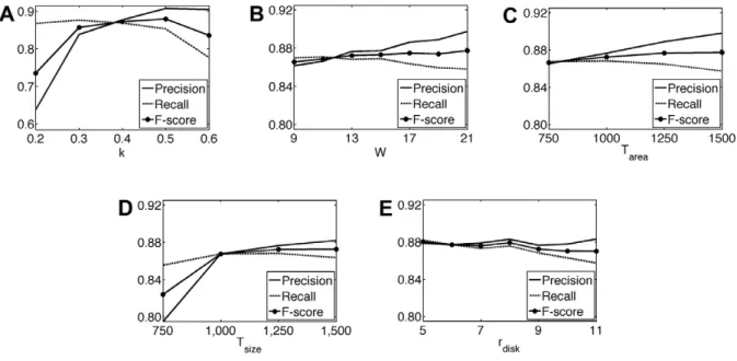
Figure 9. For the test set, the precision, recall, and F-score measures. As a function of (A) the Sobel threshold constant k, (B) the size W of the majority filter, (C) the area threshold Tarea, (D) the size threshold Tsize, and (E) the radius rdiskof the structuring element.
doi:10.1371/journal.pone.0048664.g009
Figure 10. Visual results of the proposed algorithm obtained on the images of different cell lines. doi:10.1371/journal.pone.0048664.g010
threshold. It repeats the same procedure on the resulting components, this time using a fine structuring element and a smaller area threshold. Likewise, we use the union of bright, dark, and dark-center pixels identified by our algorithm as the initial segmentation.
These algorithms also have their own parameters. Besides, the method used to obtain the initial segmentation maps introduces additional ones. In our experiments, we use a similar method to select these parameters: we first list different values for each parameter, consider different combinations of the parameter values, and select the combination that yields the maximum F-score on the training cells.
We present the quantitative results obtained on the training and test sets in Tables 1 and 2, respectively. As mentioned before, to obtain these results, we employ a marker-based evaluation method that uses a distance threshold to find matches between the markers and the actual cells. Smaller values of this threshold increases false detections and misses since some of the identified markers are not close enough to the exact centroids of the gold standard cells. This decreases one-to-one matches, giving lower precision and recall values. Its larger values increases oversegmentations since more markers are matched to the same gold standard cell. This also decreases to-one matches. Figure 7 shows the number of one-to-one matches as a function of the distance threshold value for the training set. Considering these numbers, we select the distance threshold as 30, which gives the maximum one-to-one matches for all of the algorithms. We also present the visual results obtained for example images in Figure 8.
The results show that the definition of smart markers leads to higher precision and recall values. Compared to the other algorithms, it gives more one-to-one matches with relatively less false detections and misses. In Tables 1 and 2, we observe that the most successful comparison algorithm is the intensity-based algorithm. However, when we examine the visual results (the third column of Figure 8), we observe that this algorithm usually fails in finding Type I cells, which contain bright pixels both in their centers and on their boundaries, and Type IV cells, which correspond to apoptosis. Besides, for images that contain noise and artifacts, it may find a very large number of markers. Indeed, the reported results do not reflect this fact since we mask the markers with the initial segmentation found by our algorithm. If such a masking operation was not used, the number of false detections would increase from 138 to 427.
Moreover, the results show that the distance-based and conditional-erosion algorithms give less one-to-one matches due to a high number of misses. The visual results of these algorithms (the fourth and the fifth columns of Figure 8) reveal that they are not successful in finding clumped cells, regardless of their
morphological classes. It is also worth noting that these algorithms require an initial segmentation and the quality of this segmenta-tion greatly affects the final segmentasegmenta-tion results. In the experiments, we use the initial segmentation found by our algorithm, which uses domain specific knowledge to define this segmentation. Without using this domain specific knowledge, it may be harder to find a good initial segmentation especially for Type III cells, which correspond to darker and non-circular cells, and Type IV cells, which correspond to apoptosis. This may further decrease the number of one-to-one matches.
Parameter analysis
The proposed algorithm has five model parameters. To investigate the effects of each parameter to the segmentation performance, we fix four parameters and observe the precision, recall, and F-score measures as a function of the other. In Figure 9, we present the parameter analysis performed on the test set.
There are three external parameters in the cell pixel quantiza-tion step. The first one is the Sobel threshold constant k that is used to define dark pixels. When its smaller values are used, some background pixels are also defined as dark so that false background regions are identified as cells. This increases the number of computed cells without increasing one-to-one matches, which in turn lowers precision. On the other hand, when larger values of this constant are used, less dark pixel components can be found. This leads to less computed cells as well as less one-to-one matches, which lowers recall. Note that larger values do not lower precision since the number of computed cells and one-to-one matches decrease concurrently. In our experiments, this parameter is selected as 0.4. Figure 9A shows that this selected value provides a good balance between precision and recall.
The second parameter is the size W of the majority filter that is used for alleviating the effects of noise in pixel quantization. The filter size W should be selected large enough to get the benefits of majority filtering. On the other hand, selecting too large filter sizes causes to assign incorrect labels to pixels. As seen in Figure 6B, this changes the balance between precision and recall. The area threshold Tarea is the last parameter of this step. It is used to
eliminate smaller dark components. Smaller threshold values identify more false regions as cells whereas larger values give less computed cells and one-to-one matches. These decrease precision and recall, respectively, as in the case of the parameter k. In the experiments, Tarea is selected to be 1000, which gives high
precision and recall values at the same time (Figure 9C). There are two parameters used in the smart marker extraction step. These are the size threshold Tsizeand the radius rdisk of the
structuring element. Smaller values of Tsize cause to define false
Table 3. Comparison of the marker-controlled watersheds that use the smart markers and those identified by the comparison algorithms.
Area-based Cell-based
Precision Recall F-score Precision Recall F-score Smart markers 0.73 0.67 0.70 0.83 0.77 0.80 Intensity-based 0.71 0.54 0.62 0.75 0.64 0.69 Distance-based 0.50 0.38 0.43 0.64 0.40 0.49 Cond-erosion 0.50 0.35 0.41 0.58 0.38 0.46 The results are obtained on the training set.
doi:10.1371/journal.pone.0048664.t003
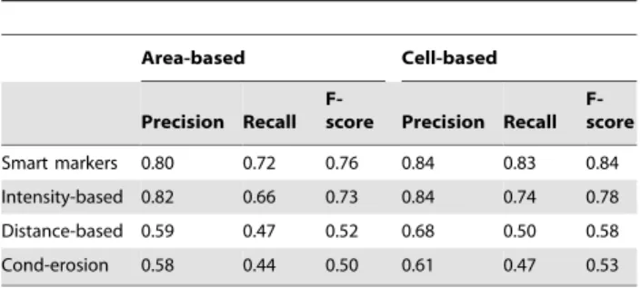
Table 4. Comparison of the marker-controlled watersheds that use the smart markers and those identified by the comparison algorithms.
Area-based Cell-based
Precision Recall
F-score Precision Recall F-score Smart markers 0.80 0.72 0.76 0.84 0.83 0.84 Intensity-based 0.82 0.66 0.73 0.84 0.74 0.78 Distance-based 0.59 0.47 0.52 0.68 0.50 0.58 Cond-erosion 0.58 0.44 0.50 0.61 0.47 0.53 The results are obtained on the test set.
markers, increasing the number of computed cells without changing one-to-one matches. On the other hand, its larger values cause to eliminate some true markers, decreasing the number of computed cells as well as one-to-one matches. These two conditions decrease precision and recall values, respectively, as observed in Figure 9D. The radius rdiskslightly changes the results
except the case when largest values are used (Figure 9E). The largest values prevent the iterative erosion algorithm to identify especially smaller true markers; this also lowers recall values. In the experiments, Tsize~1250 and rdisk~9, which give a good balance
between precision and recall.
Discussion
In this paper, we introduced the idea of defining smart markers for a marker-controlled watershed algorithm by making use of
domain knowledge specific to live cells. This definition relies on defining different pixel groups based on the morphological characteristics of the live cells and identifying the smart markers on these pixel groups. Working with 1954 KATO-3 gastric cancer cells, our experiments indicated the effectiveness of this smart marker definition in obtaining more successful results.
As seen in the visual results (Figure 8), the proposed algorithm can successfully find different types of cells. This is attributed to the fact that the algorithm uses domain specific knowledge so that it knows there exist different types of cells in a cell line (or a tissue) and the characteristics of these cells. Therefore, it can use this knowledge in defining its markers. On the other hand, the other algorithms do not use the knowledge of the existence of different cell types in a cell line. The ability of using such knowledge is indeed closely related with working on live cells. Live cells are not fully attached to the plate, and thus, cells belonging to different
Figure 11. Visual results of the watershed algorithms obtained on example images. doi:10.1371/journal.pone.0048664.g011
morphological classes can show different appearances. On the other hand, when cells are fixed, they become fully attached to the plate and their appearances become the same. The only exception is the appearance of dead (e.g., apoptotic) cells; they usually seem different than the others. Thus, to analyze the morphological classes of fixed cells, special stainings are typically required. The most of the algorithms in literature, including those that we used in our comparisons, were implemented considering fixed cells (mostly for fluorescence stained cells). This could be the reason of these algorithms not considering such kind of knowledge in their segmentations. Our proposed work is a good example of showing how domain knowledge can effectively be used in a cell segmentation algorithm.
In this work, we developed our algorithm considering the morphological characteristics of the KATO-3 human gastric cancer cell line. We also use the images of this cell line to test our algorithm. Nevertheless, it is also possible to apply this algorithm to other cell lines. To explore this possibility, we also test our algorithm on four different cell lines, namely the Huh7 human liver cancer, MCF7 human breast cancer, MFE-296 human endometrial carcinoma, and SK-BR-3 human breast cancer cell lines. The preliminary visual results obtained on example images of these cell lines are given in Figure 10. This figure shows that the results hold promise for the proposed algorithm to be also used for different cell lines. In order to obtain better results, one can consider the characteristics of these cell lines for the definition of additional pixel groups as well as for the identification of additional smart marker types on these pixel groups. This could be considered as one of the future research directions of our work. Our experiments showed that the smart marker definition increases the success in terms of marker localization. This, in turn, is expected to also increase the success of a watershed algorithm. To examine this, we implement a watershed algorithm that takes the smart markers as starting locations and grows them by using the marker types and the pixel groups (dark, dark-center, and bright pixels). Here we use the geodesic distance from a pixel to a marker boundary as the growing criterion. Let Mdark, Mcenter, and Mbright
be a set of smart markers defined on dark, dark-center, and bright pixels, respectively. In this watershed, we first grow the markers Mdark on dark pixels as long as the Euclidean and geodesic
distances from a dark pixel to the corresponding marker boundary are equal to each other. This equality constraint is defined to prevent flooding into dark pixels that belong to missing cells with unidentified markers. Then, we repeat the same procedure to grow the markers Mcenter on dark-center pixels. Finally, we
combine the grown markers with the centroid of the markers Mbrightand grow all of them on bright pixels. Here, we identify the
most distant pixels that each marker can grow into. For that, for each marker Mi, we find the first bright pixel pithat is adjacent to
background and that Mi grows into and define the maximum
distance as the geodesic distance from pito the closest boundary of
Miplus an offset value, which is set to 10 in the experiments. This
distance constraint is defined to prevent flooding into pixels of missing cells with unidentified markers as well as background pixels that are incorrectly assigned to the bright pixel group. At the end, we postprocess the results by applying the majority filter on the grown areas and filling holes in each segmented cell. For the other algorithms, we grow their markers on their initial masks by considering the same distance constraint and applying the same postprocessing.
We present area-based evaluation of these watershed algorithms for the training and test sets in Tables 3 and 4, respectively. In this evaluation, we first find the true segmented cells and then calculate the precision, recall, and F-score measures by considering the true positive pixels of these cells. A segmented cell S is said to be true if at least half of its pixels overlap a gold standard cell G and at least half of the pixels of G overlap S. That is, the pixels of a segmented cell are not considered as true positive if there is no one-to-one correspondence between this cell and a gold standard cell. In Tables 3 and 4, we also report the precision, recall, and F-score measures computed on the true segmented cells, without considering their segmented areas. Note that these cell-based results are computed on the segmented cells that are identified as true after the watershed algorithm. Thus, they are less than those computed on the markers before the watershed algorithm. This table reveals that the use of the proposed smart markers gives more successful results than the others in both area-based and cell-based evaluations. We also give the visual comparison on example images in Figure 11. When area-based and cell-based results are assessed together, one can observe that the watershed algorithm that uses the smart markers identifies cells better than finding their exact areas. To improve the segmented areas, one can combine different criteria, such as intensity and gradient values, with the pixel groups in the growing process. This would be another future research direction of this work.
Our implementation uses C for cell pixel quantization and MATLABH for smart marker extraction. The average computa-tional time for a single image is 2.63 seconds using a computer with an Intel Core 2 Duo 2.4 GHz processor and 4 GB of RAM. However, it is possible to obtain speedups by implementing the smart marker extraction step also with C. This would be considered as future work.
Author Contributions
Conceived and designed the experiments: CFK SA RCA CGD. Performed the experiments: CFK SA ID. Analyzed the data: CFK SA ID RCA CGD. Contributed reagents/materials/analysis tools: CFK SA ID RCA CGD. Wrote the paper: CFK SA RCA CGD.
References
1. Chen X, Zhou X, Wong ST (2006) Automated segmentation, classification, and tracking of cancer cell nuclei in time-lapse microscopy. IEEE Trans Biomed Eng 53: 762–766.
2. Zhou H, Mao K (2005) Adaptive successive erosion-based cell image segmentation for p53 immuno-histochemistry in bladder inverted papilloma. In: Proceedings of the 27th Annual International Conference of the Engineering in Medicine and Biology Society, 2005. IEEE-EMBS 2005. pp. 6484–6487. 3. Harder N, Mora-Bermu´dez F, Godinez WJ, Ellenberg J, Eils R, et al. (2006)
Automated analysis of the mitotic phases of human cells in 3D uorescence microscopy image sequences. In: Proceedings of the 9th international conference on Medical Image Computing and Computer-Assisted Intervention- Volume Part I. MICCAI’06, pp. 840–848.
4. Kayser G, Radziszowski D, Bzdyl P, Sommer R, Kayser K (2006) Theory and implementation of an electronic, automated measurement system for images
obtained from immunohistochemically stained slides. Anal Quant Cytol Histol 28: 27–38.
5. Kayser K, Schultz H, Goldmann T, Grtler J, Kayser G, et al. (2009) Theory of sampling and its application in tissue based diagnosis. Diagn Pathol 4: 1–13. 6. Park M, Jin JS, Xu M, Wong WSF, Luo S, et al. (2009) Microscopic image
segmentation based on color pixels classification. In: Proceedings of the First International Conference on Internet Multimedia Computing and Service. ICIMCS ’09, pp. 53–59.
7. Zimmer C, Labruyere E, Meas-Yedid V, Guillen N, Olivo-Marin JC (2002) Segmentation and tracking of migrating cells in videomicroscopy with parametric active contours: A tool for cell-based drug testing. IEEE Trans Med Imaging 21: 1212–1221.
8. Zhang B, Zimmer C, Olivo-Marin JC (2004) Tracking uorescent cells with coupled geometric active contours. In: Proceedings of the IEEE International Symposium on Biomedical Imaging: Nano to Macro, 2004. pp. 476–479.
9. Xiong G, Zhou X, Ji L (2006) Automated segmentation of drosophila RNAi uorescence cellular images using deformable models. IEEE Trans Circuits Syst Regul Pap 53: 2415–2424.
10. Malpica N, de Solorzano CO, Vaquero JJ, Santos A, Vallcorba I, et al. (1997) Applying watershed algorithms to the segmentation of clustered nuclei. Cytometry 28: 289–297.
11. Fenistein D, Lenseigne B, Christophe T, Brodin P, Genovesio A (2008) A fast, fully automated cell segmentation algorithm for throughput and high-content screening. Cytom Part A 73: 958–964.
12. Plissiti ME, Nikou C, Charchanti A (2011) Combining shape, texture and intensity features for cell nuclei extraction in pap smear images. Pattern Recognit Lett 32: 838–853.
13. Lindblad J, Wahlby C, Bengtsson E, Zaltsman A (2004) Image analysis for automatic segmentation of cytoplasms and classification of Rac1 activation. Cytom Part A 57: 22–33.
14. Wang M, Zhou X, Li F, Huckins J, King RW, et al. (2008) Novel cell segmentation and online SVM for cell cycle phase identification in automated microscopy. Bioinformatics 24: 94–101.
15. Cheng J, Rajapakse JC (2009) Segmentation of clustered nuclei with shape markers and marking function. IEEE Trans Biomed Eng 56: 741–748. 16. Jung C, Kim C (2010) Segmenting clustered nuclei using H-minima
transform-based marker extraction and contour parameterization. IEEE Trans Biomed Eng 57: 2600–2604.
17. Yang X, Li H, Zhou X (2006) Nuclei segmentation using marker-controlled watershed, tracking using mean-shift, and kalman filter in time-lapse microscopy. IEEE Trans Circuits Syst Regul Pap 11: 2405–2414.
18. Jung C, Kim C, Chae SW, Oh S (2010) Unsupervised segmentation of overlapped nuclei using Bayesian classification. IEEE Trans Biomed Eng 57: 2825–2832.
19. Adiga PU, Chaudhuri B (2001) An efficient method based on watershed and rule-based merging for segmentation of 3-D histo-pathological images. Pattern Recognit 34: 1449–1458.
20. Wahlby C, Sintorn IM, Erlandsson F, Borgefors G, Bengtsson E (2004) Combining intensity, edge and shape information for 2D and 3D segmentation of cell nuclei in tissue sections. J Microsc 215: 67–76.
21. Lin G, Chawla MK, Olson K, Guzowski JF, Barnes CA, et al. (2005) Hierarchical, model-based merging of multiple fragments for improved three-dimensional segmentation of nuclei. Cytom Part A 63: 20–33.
22. Zhou X, Li F, Yan J, Wong ST (2009) A novel cell segmentation method and cell phase identification using Markov model. IEEE Trans Inf Technol Biomed 13: 152–157.
23. Otsu N (1979) A threshold selection method from gray-level histograms. IEEE T Syst Man Cyb 9: 62–66.
24. Tosun AB, Kandemir M, Sokmensuer C, Gunduz-Demir C (2009) Object-oriented texture analysis for the unsupervised segmentation of biopsy images for cancer detection. Pattern Recognit 42: 1104–1112.