Fractional Fourier transforms and their optical
implementation. II
Haldun M. Ozaktas
Department of Electrical Engineering, Bilkent University, 06533 Bilkent, Ankara, Turkey
David Mendlovic
Faculty of Engineering, Tel Aviv University, 69978 Tel Aviv, Israel
Received March 1, 1993; revised manuscript received June 3, 1993; accepted June 10, 1993
The linear transform kernel for fractional Fourier transforms is derived. The spatial resolution and the space-bandwidth product for propagation in graded-index media are discussed in direct relation to fractional Fourier transforms, and numerical examples are presented. It is shown how fractional Fourier transforms can be made the basis of generalized spatial filtering systems: Several filters are interleaved between several frac-tional transform stages, thereby increasing the number of degrees of freedom available in filter synthesis.
Key words: optical information processing, Fourier optics, spatial filtering, correlation, graded-index media
1. FRACTIONAL FOURIER TRANSFORMS Th Fourier transform is one of the most important mathe-matical tools used in physical optics, optical information processing, linear systems theory, and some other areas. Previously, we defined fractional Fourier transforms 1-3 in
a similar spirit in which other fractional operations, such as fractional differentiation, are defined, and we showed how this operation can be optically performed with qua-dratic graded-index (GRIN) media. Here we only briefly review the notation and the basic ideas, referring the reader to the above references for details.
The ath Fourier transform of a function f(x, y) is de-noted as Sia[f(x, y)]. We require that our definition sat-isfy two basic postulates. First, 9;1f should be identical to the common Fourier transform, defined as
(0Yf)(x',y') =
f[
f: f(x,y)exp[- i2( 2 YY]dxdy (1) where s, x, x', y, and y' all have the dimensions of length. In a conventional 2f optical Fourier-transforming configu-ration,4 x and y would denote the coordinates of the input plane, x' andy' would denote the coordinates of the Fourier plane, and S2 = Af (A = wavelength of light, f = focal length of lens). The first pair of parentheses on the left-hand side of the above equation emphasizes that the vari-ables (x', y') belong to the function 91f and not tof.
Our second postulate requires that 21a(1bf) = 91a+bf.
Consistent with our two postulates, it is possible to define the fractional Fourier-transform operator physically as the operator that describes propagation along a quadratic
GRIN medium. 12
Such a medium has a refractive index profile given by'
n2(r) = n
-2[1_ (n2/nl)r2], (2)
where r = (x2 + y2)1 1 2 is the radial distance from the
opti-cal axis (measured in meters) and n1and n2are the GRIN
medium parameters. The self-modes of quadratic GRIN media are the two-dimensional Hermite-Gaussian (HG) functions, which form an orthogonal and complete basis set. The (, m)th member of this set is expressed as
'Im(X, Y) =
Vx
i,\
exp -
2 ) (3)where H, and Hm are Hermite polynomials of orders 1 and m, respectively, and w is a constant that is connected with the GRIN medium parameters. For a wavelength A, each HG mode propagates through the GRIN medium with a
different propagation constant
f6im = k[ _ 2 (n)112 + m + 1)]
(-n2) 1/2
n-
(4)where k = 2,rnl/A. We also note for future use that c = (2/k)1 2(n1/n2)114. Any function f(x, y) can be expressed in
terms of the HG basis set as
f(x,y) = E Amtm (x,Y),
I m
(5) where
Alm = X , Ax, Y)lm (X Y) dxdy,
_w _ f him (6)
with him = 21+ml! m! rw2/2.
It is worth remembering that the reason why we decom-pose the input function into HG functions is that they are the normal modes of quadratic GRIN media (just as plane waves are the normal modes of free space).
Now, consistent with the physical definition above, the fractional Fourier transform of f(x, y) of order a is defined 0740-3232/93/122522-10$06.00 © 1993 Optical Society of America
Vol. 10, No. 12/December 1993/J. Opt. Soc. Am. A 2523 mathematically as
a[f(x)] =
7
f(x)Ba(x, x')dx,9;a[f(x, y)] =
I EAj.imim(x,y)exp(i6jmaL). (7)
I mL = (/2)(n,/n 2)"2 is the distance of propagation in the GRIN medium that provides the first-order (conventional) Fourier transform. Az = aL is the distance of propaga-tion that gives the ath-order Fourier transform. It was shown' that the two postulates mentioned earlier in this section are satisfied by this definition. In the same ref-erence we also discuss and prove some of the properties of fractional Fourier transforms, such as linearity, self-imaging parameters, and intensity shift invariance.
In this paper we further investigate the fractional Fourier-transform operation. The linear transform kernel of the fractional Fourier transform is presented in Section 2. Issues of resolution and space-bandwidth product are investigated in Section 3. In Section 4 we present some computer simulations of the fractional Fourier-transform operation. Fractional Fourier trans-forms can be made the basis of generalized spatial filter-ing operations, extendfilter-ing the range of operations possible with optical information processing systems. This is discussed in Section 5. Although the fractional Fourier transform was defined in relation to GRIN media, in cer-tain cases it may be more desirable to employ bulk systems to realize them. In Section 6 we discuss how to realize a bulk system that results in the same light distribution as that of GRIN media at a finite number of planes, which will be sufficient for most applications. In the same sec-tion we also discuss other extensions and aspects that cannot be treated fully in this paper.
2. LINEAR TRANSFORM KERNEL FOR THE
FRACTIONAL FOURIER-TRANSFORM OPERATION
In order to obtain a direct expression for the ath Fourier transform of a function, we combine Eqs. (6) and (7). Let us first present the one-dimensional results. The analogs of Eqs. (6) and (7) in one dimension are
AlJ= f- hx, Wx' (8)
9ja[f(x)] = 2Ai1I'(x)exp(ifliaL), (9)
respectively, where 'ki(x) = Hi(Vx/c)exp(-x2/w2), hi
211!
\/7/V/<,
and
13 [ (n)1/2( + )] -=k -(n)I(
)
-k - X 1 (10) (11) 21) where L = (/2)(n,/n 2)"2 as in Section 1.Substituting Eq. (8) into Eq. (9), one can express the ath-order fractional Fourier transform
(0f)a(x')
aswith the transform kernel being given by
B. ( a)
exp(iBjaL)t
(,Ba (X, X') =
>
exPi
WiL\
X)
(X,)
1=0 hi Using Eq. (12), we obtain
Ba(x, x') =- - exp
ikaL-Ct) L1r
(14)
*
~~~X
exp[ (x + ]2 X exP[ ia1(T/2)1x i 1 ( )t ( X) (15)
We know that when a = 0 Eq. (13) must be equal to f(x'). In other words, we must have Bo(x, x') = 8(x - x'), the Dirac delta function. Examining Eq. (15) reveals that, apart from certain phase factors up front (which do not have any effect on the transverse profile), choosing a equal to any integer multiple of 4 results in the same kernel. {This holds because exp[-ial(w/2)] = 1 for a an integer multiple of 4.}
It is also easy to see that the kernel Ba(X, x') is not space invariant; i.e., it cannot be expressed in the form
Ba(X - x'), so that Eq. (13) cannot be reduced to a
convo-lution integral.
The fractional Fourier-transform kernel is, of course, at the same time the kernel describing propagation in qua-dratic GRIN media. As given in Section 1, the distance of propagation Az is related to a by the relation Az = aL.
Following a similar analysis, we can express the two-dimensional kernel as
Ba (x, y; x',y) 2 1 exp[ (x2 +2x2)1
X exp 2+2)1
X exp[ikaL - i - )a]
be
~~~X
Y E exP[-ita1T r/2)1 exP[- iam(,7T/2)1m 211! 2mm!
at
~~~X
H,( N/D- )H (D2 xi N/2yX
H (
'
(16)
3. RESOLUTION AND SPACE-BANDWIDTH PRODUCT
Few approximations are inherent in the propagation rela-tionships for quadratic GRIN media, which have been taken from Ref. 5. First, as is commonly done in Fourier optics, the vector nature of optical radiation has been ig-nored and a scalar theory has been employed. Second, it has been assumed that the refractive index changes little over distances of the order of a wavelength. This is valid provided that (n2/n,)A2 << 1, which, as we will see below, (13) H. M. Ozaktas and D. Mendlovic
must be always satisfied, anyway. The common slowly varying envelope approximation' has not been employed. The third approximation is to assume that the system is of infinite transverse extent. This assumption seems to contradict the fact that the refractive index must always be greater than unity [see Eq. (2)]. Of course, all real systems must be of finite extent, a fact that has several implications. First, since the Fourier transform of the function must also be represented over a finite extent, a finite number of samples is sufficient to characterize the system in the space domain. In other words, the system has a finite resolution. Another implication is that the HG modes beyond a certain order will not be relevant for our purposes because their energy content will mostly lie outside the diameter of our medium. In this section we clarify these issues, and derive the space-bandwidth prod-uct of the system.
Since it is difficult to manufacture large index varia-tions, and more fundamentally since we always have that n(r) 2 1, we must ensure that (n2/ni)r
2
<< 1 if such a system is to be realizable. Thus the parameters of our medium must satisfy
(n2/n1)(D/2)2 << 1, (17) where D is the diameter of the medium.
We will now show that if this condition is satisfied, the following consequences hold:
we obtain
(19) as the space-bandwidth product of our system. We might guess that the space-bandwidth product for a circular system would be N = (D2/4W2)2instead. Thus the mini-mum resolvable dimension is approximately given by D/(D2/&)2) = to2/D
In order to show (2) with the least amount of derivation, we will exploit the analogy with the quantum-mechanical harmonic-oscillator problem. For simplicity, we restrict ourselves to a one-dimensional discussion. In a classical harmonic oscillator the energy is given by E = khoXmax 2/2, where kho is a constant and Xmax represents the maximum
excursion from the equilibrium point. The coordinate variable x remains between the bounds -Xmax ' X ' Xma. In the quantum-mechanical harmonic oscillator the energy of the Ith eigenstate is given by El = hiWho(l + 1/2), where
1h is Planck's constant and Who is another constant.5 For
large values of I there is a correspondence between the lth eigenstate and the classical solution with the same energy E = El. Although there is always a finite probability for the absolute value of the coordinate variable to assume values greater than xmax, this probability is small for large
1. In other words, most of the probability mass of the lth eigenstate lies within the bounds
(1) The one-dimensional space-bandwidth product of the system based on sampling considerations is =D2/4w2. (2) The number of relevant HG modes (those whose energy lies predominantly within the diameter D of the medium) is =D2
/4cw2.
(3) The approximation for the propagation constant fim
[relation (4)] is valid for these modes.
To show (1), let us assume that the transverse cross sec-tion of our GRIN medium is a square with edge length D. Circular systems would probably be more common in prac-tice, but assuming a square will simplify our discussion and the results will differ from that for a circular system merely by geometrical factors of the order of unity.
Our original input function f (x, y) is necessarily bound within the transverse extent Ax = D and Ay = D. The first Fourier transform of f (x, y) is likewise bound within the spatial frequency intervals Av = D/s2and Av, = D/s2.
[s is the scale parameter appearing in Eq. (1). For a GRIN medium with parameter w this scale parameter assumes the value s = V/7r ).'] Boundedness in either domain im-plies that the meaningful information content of the sig-nal in the other domain can be recovered from its samples at the Nyquist rate.4 Thus, for instance, boundedness in the Fourier domain implies discrete samples in the space domain at intervals of 1/Avx and 1/Avy. Likewise, bound-edness in the spatial domain implies discrete samples in the Fourier domain at intervals of 1/Ax and 11Ay. The total number of samples in either domain is given by
N = NN, = (AAvx)(AyAvy) = (D2/s2)2. (18) The quantity N can also be interpreted as the number of spatial degrees of freedom of the system, or its space-bandwidth product.4 Now, using the fact that s = -7rw,
jxl ' (2E /kh.)1I2 (2hlwhl/kh.) /. (20) The eigenstates of the quantum harmonic oscillator cor-respond to the HG modes of quadratic GRIN media. The probability distributions that we have been mentioning above must now be interpreted as energy distributions. Thus, by analogy with the discussion above, we can find the bounds within which most of the energy of the Ith HG mode lies. The following relation relating the pa-rameters of the harmonic oscillator and quadratic GRIN media will easily enable us to modify the above results for our purpose5:
N/2C& = (kho/°hhI)"- (21) Using this relation in inequality (20), we obtain
jxj2• 21,2/2 = Co21. (22) Thus most of the energy of the 1th mode lies within the interval [-w\/,co<]. The modes that are relevant for our purpose are those that lie predominantly within the interval [-D/2,D/2]. Thus the largest relevant order is determined by IA/ - D/2, leading to
1 = D2/4 2. (23)
It is satisfying that the number of relevant modes is equal to the number of spatial degrees of freedom. Thus, re-gardless of whether we prefer to represent a signal f(x, y) in terms of its samples or in terms of the coefficients of its HG components, we need the same number of real numbers.
Given (1) and (2), it is easy to demonstrate (3). Since we have shown that the relevant HG orders are those with
D 2 2
Vol. 10, No. 12/December 1993/J. Opt. Soc. Am. A 2525
(a)
(b)
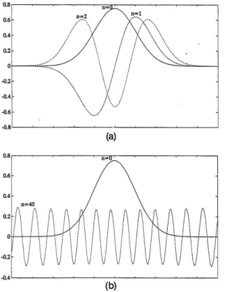
Fig. 1. Hermite-Gaussian (HG) functions of different orders n. (a) Solid curve, n = 0; dashed curve, n = 1; dashed-dotted curve, n = 2; (b) solid curve, n = 0; dashed curve, n = 40. The one-dimensional version of Eq. (3) has been plotted normalized so as to have unit energy.
1, m < D2/4602, we can write 2 n2 2(n2 1/2 2 (n21'2 2D 2 - + M + Y (+ ) < -I- & k ni nJ k ni 4 n2D2 2 << 1, (24) where the last step follows from the fact that we had as-sumed that (n2/n,)D2 << 1 for a realizable GRIN medium. Thus the approximation of 31m [see relation (4)], which is crucial in deriving the exact Fourier-transform relation-ship,' has been justified.
4. COMPUTER-SIMULATED NUMERICAL EXAMPLES OF FRACTIONAL FOURIER TRANSFORMS
In order to demonstrate the fractional Fourier-transform operation, we have carried out some computer simulations for one-dimensional signals.
First, let us illustrate the nature of the HG functions with some examples. Figure 1(a) shows the three lowest orders, and Fig. 1(b) depicts the 40th order. Note that HG functions with high order can be approximated by sinusoidal functions. The horizontal axes in all the plots in this paper, except Figs. 4 and 9, are in arbitrary units.
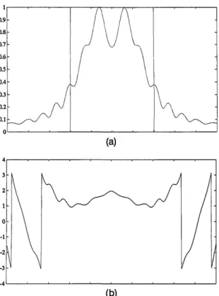
Now, let us assume that the input function is the com-mon rectangle function. Figure 2 shows this initial signal and the magnitude of its first-order Fourier form. The phase information of the first Fourier trans-form is shown in Fig. 3.
The coefficients Al appearing in Eq. (8) for our specific example are shown in Fig. 4. This figure demonstrates the fact that in this example harmonics of higher orders (>15) contain very little of the total energy.
Figure 5 shows the fractional Fourier transform of order 0.25. Note that this same distribution is also the fractional Fourier transform of orders 1.75,2.25,.... Figures 6 and 7 show the fractional Fourier transforms of our input function for the orders 0.5,1.5,... and 0.75, 1.25,..., respectively. In these figures we can observe the rectangle function evolving into the sine function as the parameter a is varied from 0 to 1.
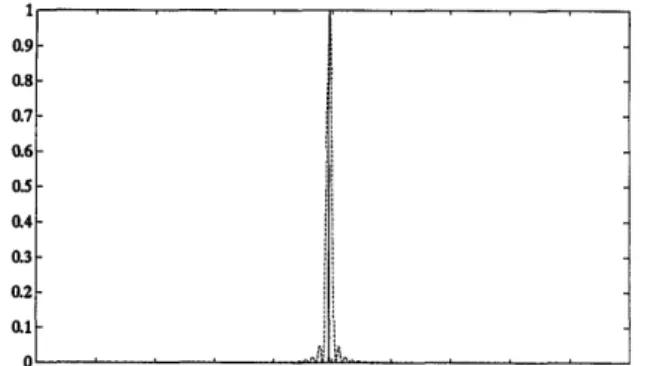
Another example that we simulated is the delta function. Figure 8 shows the input signal and its second-order Fourier transform, which is an image of the input signal. This second-order Fourier transform was calculated with Eqs. (8) and (9). One can easily explain the finite width of the output by examining Fig. 9, which is the coefficient
Fig. 2. Solid lines, input signal; dashed curve, first-order Fourier transform.
1.5 1 -0.5 .0.5 .1 -1.5 .2
Fig. 3. Phase of the first-order Fourier signal in Fig. 2.
magnitude of its
transform of the input
80 60 40 20 0 -0 10 20 30 40 50 60 70 80 90 100 HARMONIC ORDER
Fig. 4. Energy distribution among the first 100 HG orders.
IW, . . . E . . . .
-20
..
H. M. Ozaktas and D. Mendlovic
0.9
/\
/\ 0.8 I 0.6 0.5-0.4/
0.3-0.2 'N 0) (b)Fig. 5. Fractional Fourier transform of order a = 0.25. (a) Mag-nitude, (b) phase.
series Al, and noting that there is a relatively large amount of energy contained in the higher orders. This being the case, the first 100 orders that we worked with in these simulations are seen to be insufficient. Remember that in Section 3 we found that the required number of HG orders is equal to the number of resolution elements. In our simulations the number of resolution elements is 1000 pixels, so that one must calculate at least this many orders to recover the delta function at the same resolution in the second Fourier plane. Doing so was less important with the rectangle function because not so much energy was concentrated in the higher orders, so that neglecting them had a much smaller impact.
Figure 10 is the magnitude of the 0.1th fractional Fourier transform of the delta function, Fig. 11 is the 0.4th order, and Fig. 12 is the first Fourier transform (which is seen to be approximately constant as expected). In these figures we can observe the delta function evolving into the constant function as the parameter a is varied from 0 to 1. 5. GENERALIZED SPATIAL FILTERING BASED ON FRACTIONAL FOURIER TRANSFORMATIONS
Fractional Fourier transforms can form the basis of gen-eralized spatial filtering operations, extending the range of operations possible with optical information processing systems. Conventional Fourier plane filtering systems are based on a spatial filter introduced at the Fourier plane, which limits the operations achievable to linear space-invariant ones (i.e., operations that can be ex-pressed as a convolution of the input function with a space-invariant inpulse response). By introducing several filters at different fractional Fourier planes, one can
im-plement a wider class of operations. [We should note that full space-variant operations can be implemented with approaches such as (or equivalent to) vector-matrix multi-plier architectures6 or multifacet architectures,7 but these result in a heavy penalty in terms of space-bandwidth
I 0.9 0.8 0.7- 0.6-0.5 0.4-0.3 Q2 I
0.1 hi,,
\J.,
...\ ,f a,\\
,,
(a) (b)Fig. 6. Fractional Fourier transform of order a nitude, (b) phase. = 0.5. (a) Mag-0.9 0.8-0.7 I 0.5 0.4- 0.3-0.2 -/ ..-. I 0.1
~
"" / / \\./ \\ (a) (b)Fig. 7. Fractional Fourier transform of order a = 0.75. (a) Mag-nitude, (b) phase.
Vol. 10, No. 12/December 1993/J. Opt. Soc. Am. A 2527 a 0 0 0 0 0 0 0 0 .9-°8 . 06, .3 .2 . .1~~~~~~~~~~~~~~~~~~~~~~~ C1-i
Fig. 8. Solid line, input signal (delta function); dashed curve, its second-order Fourier transform.
a I 0. 0. 0, 0. 0 0 0. 0. 0. 1 eab Boseeoooloso .9 -.8 .7 .6 .5 .4 .3 .2 .1 OA -.A -.A -.A ..A -.n -.A _A _A e n U 10 ZO 0 40 0 /0 HARMONIC ORDER
Fig. 9. Energy distribution among the first the delta function.
80 90
tions at the desired planes. Such systems are described in Section 6.
Conventional 4f spatial filtering configurations are merely a very special case of the above system. Only one filter is used, and this filter is inserted at the a = 1st Fourier plane. The common 4f system is, by design, such that if the single filter is removed from the system, the output becomes identical to the input (apart from a coordi-nate inversion). That is, there is an imaging relationship between the input and output planes. However, in
gen-eral, we see no a priori reason to impose this restriction on our systems, so that the overall length of the system becomes an additional degree of freedom during design.
For notational convenience, we will work with one-dimensional signals throughout this section.
Further-more, we will represent our functions with discrete vectors with a finite number of elements. In Section 3 we showed that the one-dimensional space-bandwidth product of a fractional Fourier transformer based on a GRIN medium of transverse extent D and parameter w was given by D2/4w2. This was also the number of HG modes with a significant contribution within this diameter. Let us denote this number as N. The fact that there exists only a finite number of degrees of freedom over this finite
di-100
100 HG orders for
Fig. 10. Magnitude of the a = 0.1th-order fractional Fourier transform of the delta function.
product utilizations In this context, also see Refs. 9 and 10.]
A system for performing generalized spatial filtering would consist of a certain length of quadratic GRIN medium, followed by the first spatial filter, followed by
another length of quadratic GRIN medium, followed by the second spatial filter, and so on (Fig. 13). The effect of propagation in quadratic GRIN media has been analyzed elsewhere' and summarized in Section 1 above. The ef-fect of a spatial filter is simply to multiply the functional form of the light distribution incident upon it by its com-plex amplitude transmittance function.
One can realize such a system by cutting a certain length of quadratic GRIN medium at a finite number of places and inserting filters between the cuts. If GRIN fibers are found inconvenient to work with, it is possible to use a bulk system that produces identical light
distribu-Fig. 11. Magnitude of the a =
transform of the delta function. 0.4th-order fractional Fourier
0.9 0.8 0.7 0.6 0.5 0.4- 0.3-0.2 0.1 0
Fig. 12. Magnitude of the first-order Fourier transform of the delta function.
INPUT FILTER 1 FILTER 2 OUTPUT
GRIN GRIN 2
Fig. 13. System for performing generalized spatial filtering con-sists of several fractional Fourier transform stages with spatial filters inserted in between.
1 X | | , ;i v 0.9 0.7-0.6 0.5- 0.4- 0.3-0.2 Pi 0.1 0
ameter justifies the use of the samples of functions at ap-propriate intervals to represent the functions.
Let the function f(x) be represented by its N samples in vector form as
f =[ff2 ... fN] T. (25)
T denotes the transpose operator, i.e., f is a column vector. f will be used to denote the transverse amplitude distribu-tion of light in the GRIN medium. The distribudistribu-tion at axial location z will be denoted as f(z). If the axial loca-tion z = z is chosen as the input of our system, f(z1) will
represent the input function. After propagation by a dis-tance Az12 = 2 - z1to z2 the light distribution f(z2) will
be given by the linear relationship
f(z2) = B(Az12)f(z1), (26)
where B is an N X N matrix operator that is equal to the identity matrix 1 when Az12 = 0. The fact that B
de-pends only on Az12 and not on z1 and z2 individually is a
consequence of the fact that the system is insensitive to a shift of origin in the z direction. Another physically self-evident property is that
B(Az2 3)B(Az12) = B(Az2 3 + AZ12) = B(Az 13)- (27)
This additivity property is, by design, equivalent to the second postulate mentioned in Section 1. More generally,
f = I produces an output function directly proportional to *I. More precisely,
B(Az)I' = exp(iBAz)I', (32) where f31 is given by Eq. (12). The factor exp(i 1Az) is the
eigenvalue associated with the 1th eigenfunction.
Now, let the input function f(zi) be expanded according to Eq. (30) with coefficients Al(zl); i.e.,
f(z1) = A(zi), A(z1) = *-If(z 1).
(33) (34) On propagation from z1to z2each eigenvalue is multiplied
by the eigenvalue given above. This can be interpreted as a change in the expansion coefficient; i.e.,
A1(z2) = exp(i,1Az12)Az(z),
A(z2) = P(Az12)A(z),
(35) (36) where the diagonal matrix 13 has exp(i13IAz12) as its th
diagonal element. Now, using Eq. (30), we can write
f(z
2) = A(z2). (37) Now, combining Eqs. (34), (36), and (37), we arrive atf(z2) = T18(Az 2)Prlf(z1), (38)
so that
r B(Azii+
1) = B( Azii+l) .
(28) Evidently, B(Az) is the discrete fractional Fourier trans-form operator with order a = Az/L and will also be de-noted asBa-We now seek to find the explicit form of B in terms of previously defined quantities. Let the sampled version of the Ith member of the HG function set be denoted in vector form as *1 = [kllt2l tNz]T. Here we define
il = 'I,-/ so as to ensure that the matrix ', with *I as its columns, is not only orthogonal but also ortho-normal, and also so that the order of the HG set 1 now ranges from 1 to N rather than from 0 to N - 1. Based on the results of Section 3, f can be expanded into the first N HG functions to a good approximation (since only for these first N functions is the energy predominantly con-tained within the extent D):
N
fi = ZA*P), 1 (29)
I-1
f= A,
(30)
where Al = A11_
Vh7,
A = [A1A2... AN]T, and I is thematrix made up of the coefficients i,. The above ap-proximation is best when the coefficients Al appearing in Eq. (29) are identical to those appearing in the infinite-summation Eq. (5) (see Appendix A). Equation (30) can also be inverted to yield
A =W'1f. (31)
The columns of the matrix I are eigenmodes of the op-erator B(Az), regardless of Az. This means that applica-tion of the operator B on an input funcapplica-tion of the form
B(Az12) = I'P(AZ12
)'1-The last equation may be inverted to yield I-'B(Az2)I = B(Az12).
(39)
(40) In the parlance of matrix theory the unitary transforma-tion effected by the matrix T diagonalizes the operator B. This is to be expected, since T is constructed with the eigenvectors of B as its columns. The elements of the diagonal matrix 13 are, as mentioned above, the eigen-values of B.
Let us now discuss some properties of the above matri-ces. It is well known that the orthogonal HG set satisfies
f
Pl(xNk(x)dx = 1Akhz, (41)so that
f
+1(x)+k(x)dx = 81k. (42)If N is large, then, by the definition of Riemann integrals, the inner product
N
I
=2 filiAk
i-l (43)
is a good approximation of the previous integral, so that
'IOIk = Sik, which verifies the fact that the matrix * is
orthonormal, i.e., *T* = = 1, where 1 is the iden-tity matrix.
The formalism of this section can be interpreted in two ways. We may consider the discrete vectors as being
Vol. 10, No. 12/December 1993/J. Opt. Soc. Am. A 2529 sampled versions of continuous functions. In this case we
must bear in mind that the orthonormality of the discrete (sampled) HG function set is approximate, the approxima-tion becoming better and better as N oo. In this case it
must be assumed that N is large enough that the ortho-normality condition holds to a sufficiently good approxi-mation. Alternatively, one may choose to interpret the following as an a priori discrete approach. Then, the fractional Fourier-transform operation can be effected by multiplication of a given vector by the ath power of the discrete Fourier-transform matrix. The computation of the ath power of the discrete Fourier-transform matrix, as well as its eigenvalues and eigenvectors, is discussed in Ref. 11. In this reference it is shown that a set of eigen-vectors satisfying the orthonormality condition exactly can be found.
Since t is a real orthonormal matrix, it is also unitary (i.e., its inverse is equal to the complex conjugate of its transpose). The matrix 13 is diagonal and hence symmet-ric 'aT = 3. It is also easy to show that 18 is unitary but
not Hermitian (i.e., 18 is not equal to the complex conjugate of its transpose). Since B is a product of three unitary matrices, it is also unitary but is also not Hermitian. Moreover, it is possible to show that B is also symmetric. Using Eq. (40), the reader can analytically verify the prop-erty given in Eq. (27), as well as show that B-'(Az) = B(-Az). Another easily verified and useful property is the following: Any diagonal matrix D that commutes with B (i.e., satisfies BD = DB) is necessarily equal to the identity matrix, perhaps multiplied by a scalar constant.
Now, referring to Fig. 13, let us assume that we choose
z = z as our input plane and f(zo) as our input function.
If the first filter is located at z = z1, the functional form
of the light distribution immediately before the filter (at z = z ) will be denoted as f(z1) and
f(z1') = B(Az0 1)f(zo), (44)
where Azo1 = z1 - z. Let the continuous filter functions
be denoted as h(x) and their discrete forms as hj=
[hvha,*.. hNj] T. Since the effect of the filter is term-by-term multiplication of the components, the functional
form of the light distribution immediately after the filter (at z = zl ) can be expressed as
f(z) H1f(zT), (45)
where Hj is a diagonal matrix with its ith diagonal ele-ment given by hij. Generalizing the last two equations, we obtain
f(zJ) = B(Azj_1,j)f(z+-1), f(zJ+) = Hjf(zj-),
(46) (47)
where T denotes the overall transfer matrix of the system. Given M, zi, z2,..., ZM+1, and H1, H2,... , HM, one can
cal-culate T.
More interesting, however, is to start with a desired T, representing an arbitrary linear transformation, and syn-thesize this T by choosing the above parameters.
If T is in Toeplitz form, representing a linear operation expressible as a convolution, only one filter (M = 1) wil be sufficient. More general matrices will require a larger number of filters. The matrix T has N X N degrees of
freedom, whereas each filter has only N. Thus a system that can realize any given matrix will need to have at least N stages. Other matrices with certain
redundan-cies or special forms may be implemented with a smaller number of filters. Thus, given a matrix T, the problem is to find the smallest number of filters with which it can be realized and the corresponding filter locations and values. Since the filter locations do not represent a significant number of degrees of freedom, we may simplify by
choosing zj = jAz, where Az is a constant. Then Eq. (49) becomes
T = B(Az)HMB(Az)HMl... B(Az)HB(Az). (50) The solution of these nonlinear equations is not straight-forward and must be left out of the scope of this paper. We satisfy ourselves by identifying two problems for
fu-ture research:
(1) Solve for the minimum value of M and the compo-nents of Hj starting from a desired matrix T. It would also be useful to relate the minimum value of M to some characteristic number or order of the matrix.
(2) For a fixed number of filters M, give a general char-acterization of the T matrices that can be realized.
For completeness, we also provide the dual description of propagation through the sandwiched cascade of filters and GRIN media. Passage through a filter is most simply described in the original function space [Eq. (45)], since
Hj is a diagonal matrix. On the other hand, propagation
through a GRIN medium is most simply described in HG coefficient space, since the matrix P is diagonal. This is why we transform to HG coefficient space each time we want to propagate our function through a section of a GRIN medium. Alternatively, we may choose to construct our overall transfer function in HG coefficient space. This time we would fall back to original function space each time we want to work our way through a filter. In this case Eqs. (48) and (49) can be written in the form
(51) A(zout) = *-'TTA(Zin),
T = Wt1(AzMM+l)rHm . . t13(AZ1,2)1It1
x H1WP(Azo,1)yWIr, (52)
where j = 1, .. . , M + 1 if there are M filters for the first equation andj = 1, ... , M for the second equation. Thus the overall effect of passage through M filters can be
de-scribed as
f(zout) = f(zM+1) = Tf(zo) = Tf(zi.), (48)
T = B(AzMM+l)HMB(AzM_. 1,M)HM_1 ... B(Az1,2)H1B(Azo,1),
(49)
S = 13(AzMM+1)Gm . .13(Az1 2)GP(Azoi), (53)
where S = -'1T IV and Gj = *-'Hj*. In deriving these relations, we made use of Eqs. (30) and (39).
6. DISCUSSION AND EXTENSIONS
There are many aspects of fractional Fourier transforms and their optical implementation that we have been un-H. M. Ozaktas and D. Mendlovic
able to cover in this paper, as well as several open issues. Here we briefly mention some of these so as to point to future directions.
The definition of fractional Fourier transforms can be extended to complex orders. Optical realization of com-plex ordered transforms would involve attenuating or am-plifying media.
It would be interesting to explore what kind of fractional transformations are performed by GRIN media that have other than quadratic profiles. One can define a whole family of transformations by considering propagation in GRIN media with the refractive index profile
n
2(r) = n[1 - (n/nj)r1], (54) where p would act as an additional parameter of the trans-formation family. p = 2 corresponds to quadratic media, which we have analyzed.As we mentioned in Section 5, a detailed treatment of how many filters are needed and how they should be syn-thesized to realize a given operation must be postponed for future study. Here we must satisfy ourselves by not-ing that this process, which in its extreme constitutes a generalization of conventional planar spatial filtering to volume spatial filtering, would ultimately be limited by noise and scatter from the several spatial filters.
It is worth making several additional comments about the generalized spatial filtering process:
(1) The system can be optically implemented with many pieces of a GRIN medium in cascade, with spatial filters sandwiched between them. However, GRIN media tend to have rather low space-bandwidth products. For this reason a bulk optics implementation of fractional Fourier transforms may be desirable. Two options are suggested. The first is to directly implement Eqs. (6) and (7). An ordinary optical correlator can be used to calculate the Alm parameters [Eq. (6)], and then, with a mask and another correlator, we can reconstruct 9;0[f(x,y)] [Eq. (7)]. This is a very complicated configuration. The second option, which is based on a recent alternative definition for the fractional Fourier transform, is more provocative.3 This definition employs Wigner distributions. The ath frac-tional Fourier transform is defined as follows:
Treat the Wigner distribution of a one-dimensional function as a two-dimensional function and rotate it by a(ir/2) rad. The unique function (apart from a constant phase factor) having this Wigner distribution is the ath Fourier transform of the original function.
Based on the fact that a rotation of the Wigner distribu-tion can be achieved simply with a system involving free-space propagation followed by a lens and then another free-space propagation, a bulk optics implementation of this definition of the fractional Fourier transform was suggested.3 Elsewhere we show that both definitions are equivalent,12 so that this system can be used in our
gener-alized spatial filtering configuration.
(2) Generalized spatial filtering need not involve frac-tional Fourier transforms. One can cascade several con-ventional first-order filtering stages and investigate the range of operations possible under this restriction. Doing
so results in a special case of our formalism with Az = L for all the stages.
(3) Generalized spatial filtering need not utilize the fractional Fourier transform as we have defined it. For instance, one can simply take any conventional imaging system and insert spatial filters at any number of inter-mediate planes. A similar matrix formulation would be possible in this case as well, although it would not be so elegant, as such systems are not uniform in the longitu-dinal direction. (For a comparison of conventional 2f Fourier-transform configurations with GRIN-based sys-tems, see Ref. 1.)
(4) An interesting question is the following: What is the minimum physical distance between two consecutive filters? In other words, what is the total number of filters that we can use simultaneously in a system with given overall length? The answer to this question should be re-lated to the depth of focus of the system.
7. CONCLUSION
We derived the linear transform kernel for fractional Fourier transforms. We then discussed the spatial reso-lution and the space-bandwidth product for propagation in GRIN media in direct relation to fractional Fourier transforms and also presented some simple numerical ex-amples. We showed how fractional Fourier transforms can be made the basis of generalized spatial filtering systems. In conventional optical spatial filtering systems the longitudinal dimension is wasted. We have suggested that this idle dimension be used by introducing many con-secutive filters, thereby increasing the number of degrees of freedom available in filter synthesis.
APPENDIX A
Let the function f (x) be expanded in terms of the basis set TW(x) as follows: f(x) =
AltP
(,
1=0Al
= fxx) dx. (Al) (A2) Now let f(x) be approximated by the finite summationN-1
f(x) = 2 CIIPI .
1=0
Then the mean-square error
f (x) -
E
CjI (x)exp(
(A3)
(A4) is minimized by the choice of Cl = A1.13
ACKNOWLEDGMENTS
Some of the ideas in this paper were developed during in-tensive study sessions organized by Adolf W Lohmann at the Applied Optics Group of the University of Erlangen-Nirnberg during the summer of 1992. We would also like to thank Ergiin Yalgin of Bilkent University for various
H. M. Ozaktas and D. Mendlovic
mathematical contributions to Section 5. David Mendlovic acknowledges a MINERVA fellowship, and Haldun M. Ozaktas acknowledges an Alexander von Humboldt fellow-ship that made this cooperation possible.
REFERENCES
1. D. Mendlovic and H. M. Ozaktas, "Fractional Fourier trans-forms and their optical implementation. I," J. Opt. Soc. Am. A 10, 1875-1881 (1993).
2. H. M. Ozaktas and D. Mendlovic, "Fourier transforms of frac-tional order and their optical interpretation," Opt. Commun.
101, 163-169 (1993).
3. A. W Lohmann, "Image rotation, Wigner rotation, and the fractional Fourier transform," J. Opt. Soc. Am. A 10, 2181-2186 (1993).
4. A. W Lohmann, "The space-bandwidth product, applied to spatial filtering and holography," Research Paper RJ-438 (IBM San Jose Research Laboratory, San Jose, Calif., 1967). 5. A. Yariv, Quantum Electronics, 3rd ed. (Wiley, New. York,
1989), Chap. 2, pp. 18-26; Chap. 6, pp. 106-127.
6. J. W Goodman, A. R. Dias, and L. M. Woody, "Fully parallel,
Vol. 10, No. 12/December 1993/J. Opt. Soc. Am. A 2531 high-speed incoherent optical method for performing discrete Fourier transforms," Opt. Lett. 2, 1-3 (1978).
7. S. K. Case, P. R. Haugen, and 0. J. L0berge, "Multifacet holo-graphic optical elements for wave front transformations," Appl. Opt. 20, 2670-2675 (1981).
8. D. Mendlovic and H. M. Ozaktas, "Optical-coordinate trans-formations and optical-interconnection architectures," Appl. Opt. 32, 5119-5124 (1993).
9. H. I. Jeon, M. A. G. Abushagur, A.A. Sawchuk, and B. K. Jenkins, "Digital optical processor based on symbolic substi-tution using holographic matched filtering," Appl. Opt. 29, 2113-2125 (1990).
10. M. W Haney and J. J. Levy, "Optically efficient free-space folded perfect shuffle network," Appl. Opt. 30, 2833-2840 (1991).
11. B. W Dickinson and K. Steiglitz, "Eigenvectors and functions of the discrete Fourier transform," IEEE Trans. Acoust. Speech Signal Process. ASSP-30, 25-31 (1982).
12. D. Mendlovic, H. M. Ozaktas, and A. W Lohmann, "The ef-fect of propagation in graded index media on the Wigner dis-tribution function and the equivalence of two definitions of the fractional Fourier transform," submitted to Appl. Opt. 13. G. Arfken, Mathematical Methods for Physicists, 3rd