Physically-based animation of elastically deformable models

SiCAlLY - BASEÖ Â SilA ïiaS OF

ішж ті шшшшштііл

Г U Г\ С ^ д Ύ ?іѵ ^

^,? ! '** /* '"“J“-1 ■ .”î··,'· ιί^'Ί ■·’ι'^ Ч 'í<'Á ** .Τ' /^’

«* » .--.**'■ J ι , ^ ч ί ^,1 ·► - · ·—>■ ѵ'ѵ(Ч W · · · .i β « ^ .« 0 .· ¿ .,;^ ·

^Γ. i Ѵ :, -.Гѵ ·;i:¿ _ ;i¿ a íÍírrí!« ÍÍií'G

ѵ^'4.Ж',>Д.Т.^ѵЛ‘^ѵ'' ^"'*···· ^ ѵ'·'

í.*iD ΤΗ5 !H ';?i‘'ÿ T :

Cíír ООУ УШ $іЖ ^$ій£?:П'У

PHYSICALLY-BASED ANIMATION OF

ELASTICALLY DEFORMABLE MODELS

A DISSERTATION SUBMITTED TO

THE DEPARTMENT OF COMPUTER ENGINEERING AND INFORMATION SCIENCE

AND THE INSTITUTE OF ENGINEERING AND SCIENCE OF BILKENT UNIVERSITY

IN PARTIAL FULFILLMENT OF THE REQUIREMENTS FOR THE DEGREE OF

DOCTOR OF PHILOSOPHY

by

Ugur Giidiikbay

February 1994

T ñ

■G8a І39Ц

0 Copyright 1994

by

Uğur Güdükbay

and

I certify that I have read this thesis and that in my opinion it is fully adequate, in scope and in quality, as a dissertation for the degree of doctor of philosophy.

Prof. Bülent Özgüç (Principal Advisor)

I certify that I have read this thesis and that in my opinion it is fully adequate, in scope and in quality, as a dissertation for the

I certify that I have read this thesis and that in my opinion it is fully adequate, in scope and in quality, as a dissertation for the degree of doctor of philosophy.

I certify that I have read this thesis and that in my opinion it is fully adequate, in scope and in quality, as a dissertation for the degree of doctor of philosophy.

Assoc. Prof. Varol Akman

I certify that I have read this thesis and that in my opinion it is fully adequate, in scope and in quality, as a dissertation for the degree of doctor of philosophy.

Prrf. Cevdel

Assist. Prof. Cevdet Aykanat

Approved by the Institute of Engineering and Science:

Prof. Mehmet Be

ABSTRACT

PHYSICALLY-BASED ANIMATION OF

ELASTICALLY DEFORMABLE MODELS

Uğur Güdükbay

Ph.D. in Computer Engineering and Information Science

Supervisor: Prof. Bülent Özgüç

February 1994

Although kinematic modeling methods are adequate for describing the shapes of static objects, they are insufficient when it comes to producing realistic an­ imation. Physically-based modeling remedies this problem by including forces, masses, strain energies, and other physical quantities. The behavior of physically- based models is governed by the laws of rigid and nonrigid dynamics expressed through a set of equations of motion. In this thesis, we describe a system for the animation of deformable models. A spring force formulation for animating deformable models is also presented. The animation system uses the physically- based modeling methods and the approaches from elasticity theory for animating the models. Three different formulations, namely the primal, hrjhrid, and the

spring force formulations, are implemented so that the user could select the suit­

able one for an animation, considering the advantages and disadvantages of each formulation. Collision of the models with impenetrable obstacles and constrain­ ing model points to fixed positions iii space are implemented.

K eyw ords: Physically-based modeling, deformable models, animation, simulation, constraints, collision detection, collision response, partial differential equations, linear system solver.

ÖZET

ELASTİK OLARAK DEFORME EDİLEBİLEN MODELLERİN

FİZİĞE DAYALI ANİMASYONU

Uğur Güdükbay

Bilgisayar Mühendisliği ve Enformatik Bilimleri Bölümü

Doktora

Tez Yöneticisi: Prof. Dr. Bülent Özgüç

Şubat 1994

Kinematik modelleme yöntemleri nesnelerin şekillerini tanımlamakta yeterli ol­ makla beraber gerçeğe uygun animasyon üretmek sözkonusu olduğunda yetersiz kalmaktadır. Fiziğe dayalı modelleme yöntemleri bu sorunu kuvvet, kütle, en­ erji, v.b. büyüklükleri kullanarak çözmektedir. Fiziğe dayalı modellerin hareketi rijit ve rijit olmayan dinamik yasaları ile belirlenmiştir. Hareket denklemleri bu modellerin dinamik hareketini tanımlar. Bu çalışmada rijit olmayan (deforme edilebilen) modellerin animasyonu için geliştirilmiş bir sistem anlatılmaktadır. Bu sistem, modellerin animasyonu için fiziğe ve elastisite kuramına dayanan yaklaşımları kullanmaktadır. Aynı zamanda, deforme edilebilen nesnelerin ani­ masyonu için yeni bir yöntem (“yay kuvvet yöntemi”) geliştirilmiştir. Animasyon sisteminde “primal”, “hibrid”, ve “yay kuvvet” yöntemleri kullanılarak modeller hareket ettirilmektedir. Bu yolla kullanıcı yöntemlerin avantaj ve dezavanta­ jlarına göre modele uygun olan yöntemi seçebilmektedir. Modellerin sabit en­ gellerle çarpışması ve modeller üzerindeki bazı noktaların hareketinin kısıtlanması gibi seçenekler animasyonlarda kullanılabilmektedir.

A n a h ta r sö zcü k ler: Fiziğe dayalı modelleme, deforme olabilen modeller, animasyon, benzetim, kısıtlamalar, çarpışma tespiti, çarpışma sonrası hareket, kısmi türevsel denklemler, doğrusal denklem sistemi çözücüsü.

Acknowledgements

I would like to express my deepest gratitude to Prof. Biilent Özgüç for his supervision, encouragement, and invaluable advice in all steps of the development of this work. It is my extraordinary chance to work with him throughout my graduate study, to be instructed and trained in all aspects of the research.

I appreciate Prof. Yılmaz Tokad of the Eastern Mediterranean University for his valuable discussions on the implementation of deformable models, and for his motivating advice on my research. I would like to thank to Assoc. Prof. Varol Akman for carefully reading my papers, proposal, and thesis and offering various suggestions.

I also appreciate Murat Aktıhanoğlu for the shading program, and Aydın Ramazanoğlu for his help in producing the color photographs.

I am grateful to Faruk Polat, Ismail Hakkı Toroslu, Veysi işler. Özlem Özgü, and Erkan Tın, for their continuous encouragement in all stages of this study, and to Bilge Aydın, secretary of the CEIS Department, for her logistical support, and to all members of the CEIS Department for their contributions in one way or another through formal and informal discussions.

Finally, my sincere thanks are due to my family for their continuous moral support throughout my graduate study.

C ontents

1 Introd uction 1

1.1 Application Areas for Animation .3

1.2 Deformable M o d e ls... 3

1.3 The Organization of the T h e s i s ... 5

2 C onstraint-B ased M ethod s for A nim ation 6 2.1 The Uses of Constraints 8 3 C ollision D etection and R esponse 10 3.1 Collision Detection A lgorithm s... 11

3.1.1 Collision Detection for Flexible Surfaces ... 12

3.1.2 Collision Detection for Convex Polyhedra... 12

3.2 Collision Response A lgorithm s... 12

3.2.1 Analytical Collision Response A lgorithm s... 13

3.2.2 Penalty (Spring) Methods for Collision Response 13 4 N onrigid M odels 14 4.1 Formulation of Deformable M o d e l s ... 15

4.1.1 Primal Form ulation... 15

4.1.2 Hybrid Form ulation... 18

4.2 Implementation of the Primal F o rm u latio n ... 20

4.3 Spring Force Formulation for Deformable Models ... 27

4.3.1 Implementation of the Spring Force Form ulation... 30

4.4 Comparison of the Form ulations... 33 iv

4.5 Other Methods for the Animation of Nonrigid M o d els... 37

5 Sim ulation E xam ples 41

5.1 Simulation Examples Using Primal and Hybrid Formulations . . . 41 5.2 Simulation Examples Using Spring Force F orm ulation... 42

6 C onclusions and Further Research Areas 63

6.1 Contributions of the Thesis 64 6.2 Future Research D irections... 65

B ibliography 66

A p p en d ix

A T he Im p licit Functions for the O bstacles 72

B T he E xternal Spring Force Expressions 74

B .l The External Spring Force Expressions for the Boundaries . . . . 74 B.2 The External Spring Force Expressions for the C o r n e r s ... 75

List o f Tables

4.1 Preprocessing and processing times using the primal formulation. 33 4.2 Preprocessing and processing times using the hybrid formulation. 34 4.3 Preprocessing and processing times using the spring force formu­

lation 34

List o f Figures

2.1 A bead sliding freely on a rigid wire... 7

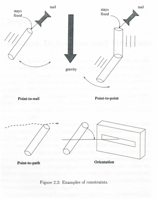
2.2 Examples of constraints... 9

4.1 Geometric representation of a deformable body for primal formu­ lation... 16

4.2 Geometric representation of deformable models for hybrid formu­ lation... 19

4.3 The band structure of the stiffness matrix K ... 23

4.4 Screen dump during the specification of the parameters for an animation... 24

4.5 Numbering of the grid... 27

4.6 Interactions (couplings) between grid points (general case)... 30

4.7 Interactions (couplings) between grid points (boundaries). 31 4.8 Interactions (couplings) between grid points (corner points). . . . 32

4.9 Preprocessing times using different formulations... 35

4.10 Processing times of one frame using different formulations... 36

5.1 A highly nonrigid surface, constrained from its four corners, falls. 43 5.2 A highly nonrigid surface, constrained from its center of mass, falls. 44 5.3 A piece of paper, constrained from three corners, applied a down­ ward force... 45

5.4 A highly nonrigid surface collides with an ellipsoid... 46

5.5 A highly nonrigid surface collides with a toroid... 47

5.6 Shaded version of the simulation in Fig. 5.1... 48

5.7 Shaded version of the simulation in Fig. 5.2... 49

5.8 Shaded version of the simulation in Fig. 5.3... 50

5.9 Shaded version of the simulation in Fig. 5.4... 51

5.10 Shaded version of the simulation in Fig. 5.5... 52

5.11 Different elastic surfaces, constrained from three corners, fall. . . . 53

5.12 Different elastic surfaces, constrained from four corners, fall. . . . 54

5.13 Different elastic surfaces, constrained from the center of mass, fall. 55 5.14 A strechy sheet, constrained from its three corners, falls... 56

5.15 A strechy sheet, constrained from its four corners, falls... 57

5.16 A strechy sheet, constrained from its center of mass, falls... 58

5.17 A piece a cloth collides with an impenetrable ellipsoid... 59

5.18 A strechy sheet drops over a toroid... 60

5.19 An elastic surface drops over a toroid with a small hole... 61 5.20 A small elastic surface passes through a toroid. 62

C hapter 1

In trod u ction

The use of computer graphics and numerical methods for three-dimensional de­ sign and modeling provides an interactive environment in which designers can formulate and represent shapes of objects. Modeling the shapes as a compo­ sition of geometrically and algebraically defined primitives, simulating scenes with shading and texture, and producing usable design images are the most im­ portant requirements for application areas such as Computer-Aided Design and Computer-Aided Manufacturing.

Currently, most of the methods used for modeling are kinematic. This be­ comes a major drawback when we want to create realistic animation since these methods are passive; they do not interact with each other or with external forces. The behavior and form of many objects are determined by the objects’ gross physical properties. For example, how a cloth drapes over objects is determined by the surface friction, the weave, and the internal stresses and strains generated by forces from the objects. As another example, a chain suspended between two poles hangs in an arc determined by the force of gravity and the forces between adjacent links that keep the links from separating.

To achieve realism in animation a model should be able to follow pre-defined paths while still moving in an interesting manner and interacting with other models as real physical objects would do. To build and animate active mod­ els, physically-based techniques should be used. These techniques facilitate the

CHAPTER 1. INTRODUCTION

creation of models capable of automatically synthesizing complex shapes and re­ alistic motions that are attainable only by skilled animators. Physically-based

■modeling achieves this by adding physical properties to the models [23]. Such

properties may be forces, torques, velocities, accelerations, kinetic and potential energies, and heat. Physical simulation is then used to produce animation based on these properties. To this end, solution of the initial value problems is required so that the course of a simulation is determined by objects’ initial positions and velocities, and by the forces and torques applied to the object along the way.

Physical simulation alone is not enough since the animator also wants to “control” the motion of objects so that he can specify the goals of motion, the way motion should be performed, and so on. Physical simulation produces impressive results, but is difficult to control since an animator cannot easily establish an intuitive link between the parameters of a simulation and the resulting motion. Besides, physiciil simulation is computationally expensive. Due to these reasons, it is not in wide use. However, researchers continue to present faster and simpler formulations to build and control the motion of models [3, 12, 45, 47]. Some of the proposed methods are related to the animation* of models composed of parts which are connected by joints, namely articulated bodies (such as humans and robots) [2, 4, 15, 18, 29, 31, 43].

Constraints provide a unified method to build objects and animate them [26].

The models assemble themselves as the elements move to satisfy the constraints. Geometric constraints, namely attachment constraints, are used to create com­ plex models from primitive bodies. In other words, they model the joints between the links of a complex model. There are other constraints, such as “point-to- path” constraints, which can be used to control the motion of the models. Such constraints are also called “kinematic constraints.”

1.1

A p p lica tio n A reas for A n im a tio n

Animation covers all changes that have a visual effect, which are time-varying po­ sition {motion dynamics)^ shape, color, transparency, structure, and texture of cin object {update dynamics), and changes in lighting, camera position, orientation, and focus, and even changes of rendering technique.

The most important application areas of animation are the entertainment industry, education, industrial applications such as control systems and flight simulators for aircraft, and scientific research. The animations in scientific visu­ alization (scientific applications of computer graphics) are generated from simu­ lations of scientific phenomena. The results of the simulations may be large data sets representing 2D or 3D data (e.g., in the case of fluid-flow simulations); these data are converted into images that then constitute the animation. At the other extreme, the simulation may generate positions and locations of physical objects, which must then be rendered in some form to generate animation. This hap­ pens, for example, in chemical simulations where the position and orientation of the various atoms in a reaction may be generated by simulation, but the anima­ tion may show a ball-and-stick view of each molecule, or may show overlapping smoothly shaded spheres representing each atom. In some cases, the simulation program will contain an embedded animation language so that the simulation and the animation proceed simultaneously.

1.2

D eform ab le M od els

CHAPTER 1. INTRODUCTION 3

An important aspect in realistic animation is modeling the behavior of deformable

objects. To simulate the behavior of deformable objects, we should approximate

a continuous model by using discretization methods, such as finite difference and finite element methods. For finite difference discretization, a deformable object could be approximated by using a grid of control points where the points are allowed to move in relation to one another. The manner in which the points are allowed to move determines the properties of the deformable object. Simulating

CHAPTER 1. INTRODUCTION

the physical properties (such as tension and rigidity), static shapes exhibited by a wide range of deformable objects (including string, rubber, cloth, paper, and flexible metals) can be modeled. For example, to obtain the effect of an elastic surface, the grid points are connected by springs. The physical quantities cited earlier should be used to simulate the dynamics of these objects. Various researchers [11, 16, 32, 30, 37, 36, 44] presented discrete models which are based on elasticity and plasticity theory and use energy fields to define and enforce constraints for modeling and animating deformable objects.

This thesis presents a new formulation for the animation of deformable mod­ els, called the spring force formulation. In other formulations based on elasticity theory [primal and hybrid formulations), the elastic properties of the materials are stored in the stiffness matrix. However, the formation of the stiffness ma­ trix automatically is very difficult and sometimes it becomes impossible to solve the differential equations for animating the models because of the numerical ill- conditioning problems. In this formulation, instead of forming the stiffness matrix automatically, elastic forces are represented as external spring forces. Although handling the elasticities using the stiffness matrix approach is elegant and the most suitable way, our approach is more effective and very fast.

An animation system which is implemented for the animation of nonrigid (deformable) models is also discussed. The system is built on top of a modeling system for representing 3D free-form objects, that uses superquadrics [6] and Bezier surfaces [9] as modeling techniques, and regular deformations [7] and Free- Form Deformations [34] for deforming these models to obtain irregular, free-form objects [25, 21]. The static models obtained by these methods can be animated using the techniques discussed in this thesis. The system is implemented using the C language [19] on a Unix^ workstation (Sun-3 or Sparc). The implementation uses the facilities provided by Sun View^ system such as windows, panels, and menus [24, 22].

tUnix is a registered trademark of AT&T Bell Laboratories. tSun View [17] is a registered trademark of Sun Microsystems, Inc.

CHAPTER 1. INTRODUCTION

1.3

T h e O rganization o f th e T h esis

In Chapter 2, constraint-based methods for animation are discussed. Different uses of constraints are also given.

In Chapter 3, the collision detection and response problem is explained. Dif­ ferent algorithms to solve this problem are discussed together with their applica­ bility to rigid, flexible, and articulated bodies.

In Chapter 4, a short description of the methods proposed by Terzopoulos et al. [37, 36, 38] for elastically deformable models is presented. Then, the imple­ mentation details of these methods in the context of our system, and algorithmic solution of the problems, such as collision of flexible models with impenetrable obstacles, are explained. A spring force formulation for animating deformable models is also presented together with its implementation details. Different for­ mulations are compared to each other in terms of their processing times and their ability to model elastic properties.

In Chapter 5, some simulation results representing the features of our system are presented.

C hapter 2

C onstraint-B ased M eth od s for

A n im ation

A good deal of research has been done towards the use of constraint methods to create realistic animation [45, 46, 47, 32]. Many constraint-based modeling sys­ tems have been developed, including constraint-based models for human skeleton [4] (in which the connectivity of segments and limits of angular motion on joints are specified), the dynamic constraints [8], and the energy constraints [44].

Constraints provide a way to specify the behavior of physical objects in ad­ vance without specifying their exact positions, velocities, etc. In other words, constraints are partial descriptions of the objects’ desired behavior. So given a constraint, we must determine the forces to meet the constraint and then find forces to maintain the constraint. For example, consider a bead sliding freely on a rigid wire (Fig. 2.1). The behavior of the bead can be described by the fact that it will stay on the wire during its motion no m atter what forces act on it. To keep the bead on wire during its motion, a constraint force fc must be applied. If fa is the force applied to the bead at any time and fc is the constraint force then the total force f = f^ + f^ = kt where t is the tangent vector to the wire. In other words, fc is the force to be added to the applied force to make the bead accelerate in a manner consistent with the constraint.

CHAPTER 2. CONSTRAINT-BASED METHODS FOR ANIMATION

Figure 2.1: A bead sliding freely on a rigid wire.

constraints that the parts of a model are supposed to satisfy. A model may be

underconstrained, in which case there are additional degrees of freedom that the

modeler can adjust (e.g., the location of the point of contact of a sphere and a cube), or overconstrained, in which case some of the constraints may not be satisfied (which could happen if both the top and bottom of the sphere were constrained to lie on the top face of the cube). In constraint-based modeling, the constraints must be assigned a priority, to satisfy the most important constraints first.

In energy-constraint systems, constraints are represented by functions that are nonnegative everywhere, and are zero exactly when the constraints are satisfied. (These are functions on the set of all possible states of the objects being modeled.) These are summed to give a single function E. A solution to the constraint problem occurs at a state for which E is zero. Since zero is minimum for E (its component terms are all nonnegative), such states can be located by starting at any configuration and altering it so as to reduce the value of E. The minimum is found by way of numerical methods.

The specification of constraints is complex. Certain constraints can be given by sets of mathematical equalities (e.g., two objects that are constrained to touch at specific points), or by sets of inequalities (e.g., when one object is constrained to lie inside another). Other constraints are more difficult to specify. For example, constraining the motion of an object to be governed by the laws of physics re­ quires the specification of a collection of differential equations. Such constrained systems, however, lie at the heart of physically-based modeling.

CHAPTER 2. CONSTRAINT-BASED METHODS FOR ANIMATION

2.1

T h e U ses o f C on strain ts

Constraints can be used for different purposes in animation (cf. Fig. 2.2) [8]: • Point-to-nail constraint: This is used to fix a point on a model to a user-

specified location in space. The body can make a pendulum motion about the constrained point, but the constrained point may not move.

• Point-to-point (attachment) constraint: This is used to attach two points on different bodies to create complex models from simpler ones. In other words, attachment constraints model the joints between bodies. The bodies may move around freely, as long as the two constrained points stay in contact. • Point-to-path constraint: This type of constraint requires some points on

a model to follow an arbitrary user-specified path (a trajectory which is specified as a function of time). Here, the rest of the body is allowed to move according to the forces and torques acting on the body.

• Orientation constraint: This type of constraint is used to align objects by rotating them. •

• Other constraints, such as point-on-line which restricts a point to move on a given line, sphere-to-sphere which requires two spheres to touch while sliding along each other, etc.

CHAPTER 2. CONSTRAINT-BASED METHODS FOR ANIMATION 9

nail nail

Point-to-nail Point-to-point

C hapter 3

C ollision D etectio n and R esp on se

When several objects are involved in a computer animation at once, the prob­ lem of detecting and controlling object interactions is encountered. In such an animation, we may have more than one object moving around, or we may have impenetrable obstacles (such as walls) that do not move. When no special atten­ tion is paid to object interactions, the objects will sail through each other; this is usually not physically reasonable and produces a disconcerting visual effect. Whenever two objects attem pt to interpenetrate each other (i.e., the surface of one object comes into contact with the surface of a second object), a collision is said to occur [5, 28].

The general requirement that arises then is an ability to detect collisions. Most animation systems at present do not provide even minimal collision detection, but require the animator to visually inspect the scene for object interactions and re­ spond accordingly. This is time consuming and difficult even for keyframe or parameter systems where the user explicitly defines the motion; it is even worse for procedural and dynamical animation systems where the motion is generated by functions and laws defining their behavior. Although automatic collision de­ tection is expensive to code and to run, it is a considerable convenience for an­ imators, particularly when more automated methods of motion control, such as dynamics or behavioral control, are used.

The other related issue is the response to a collision once it is detected. Even keyframe systems could benefit from automatic suggestions about the motion

CHAPTER 3. COLLISION DETECTION AND RESPONSE 11

of objects immediately following a collision; animation systems using dynamic simulation inherently must respond to collisions automatically and realistically. Linear and angular momentum must be preserved, and surface friction and elas­ ticity must be reasonable. Collision response algorithms can be classified into two groups:

• Analytical methods^ which are limited to rigid and articulated objects, are typically faster. Analytical algorithms could be used within a kinematic animation system.

• Penalty, or spring methods, which introduce restoring spring forces when objects inter-penetrate each other. These methods are more general, work­ ing equally well for flexible, rigid, and articulated bodies. They could not be used within a kinematic animation system since they assume the ability to use the dynamics equations of motion to predict the motion immediately after impact.

In the following, collision detection and response algorithms are explained in detail.

3.1

C ollision D e te c tio n A lgorith m s

Collision detection involves determining when objects penetrate each other. It is clearly an expensive operation, particularly when large numbers of objects with complex shapes are involved. Another issue is the ability to detect simultane­ ous collisions (multiple contacts at the same time). Furthermore, two objects may collide in such a way that a region, rather than a set of isolated points, may contact. Collision detection has been extensively pursued in the fields of CAD/CAM and robotics [1]. Some of the proposed algorithms solve the problem in more generality (and at higher cost), and some others do not easily produce the collision points and the normal directions necessary if collision response is to be calculated. Finally, many collision detection algorithms are quite intricate and must deal with assorted special cases.

CHAPTER 3. COLLISION DETECTION AND RESPONSE 12

3.1.1

C o llisio n D e te c tio n for F le x ib le Surfaces

Flexible surfaces are generally modeled as a grid of points which are connected to form quadrilaterals or triangles. Collisions between surfaces are detected by testing for penetration of each vertex point through the planes of any triangle, or quadrilateral, not including that vertex (thus, self-intersection of surfaces is detected). Initially, the surfaces should be assumed disjoint. For each time step of animation, the positions of points at the beginning and at the end of the time step must be compared to see if any point went through a triangle, or quadrilateral, during that time step. If so, a collision has occurred. Consequently, the time complexity of such an algorithm is 0{nm ) for n triangles, or quadrilaterals, and m points. A correct test must consider edges and triangles, as polyhedral objects can collide edge-on without any vertices being directly involved. However, in many cases merely testing points versus triangles produces acceptable results.

3 .1 .2

C o llisio n D e te c tio n for C on vex P o ly h ed ra

The detection of collisions between solids (or closed surfaces) that have a distin­ guishable inside and outside could be treated somewhat differently. The objects’ implicit (inside-outside) functions can be used for detecting collisions. We have used this approach in our animation system to detect the collisions of deformable models with impenetrable obstacles.

A very important problem with collision detection algorithms is that they may fail to detect a collision if one object moved entirely through another during a single time step. To minimize the frequency of occurrence of such a failure, time steps should be reduced; this is the case in dynamic animations.

3.2

C ollision R esp o n se A lgorith m s

After detecting collisions between two objects, the objects should move in a physically correct manner. Collision response algorithms are developed to achieve this goal.

CHAPTER 3. COLLISION DETECTION AND RESPONSE 13

3.2.1

A n a ly tic a l C ollision R esp o n se A lg o rith m s

An analytical solution for the collision of two arbitrary objects depends on the conservation of momentum during a collision, and results in a new angular and linear velocity for each body [5]. Thus, such a solution bypasses the question of collision forces and can be used independent of dynamic simulation, assuming information concerning the body’s mass and mass distribution is provided. Ana­ lytical solutions are typically faster for strong collisions, because the solution need only be found once. However, for gentle collisions, such as a body resting quietly on top of another, spring solutions may be desirable. An important deficiency of analytical methods is that they are not suitable for flexible bodies.

3 .2 .2

P e n a lty (S p ring) M e th o d s for C ollision R esp o n se

Penalty methods introduce restoring forces when objects inter-penetrate each other [37, 44]. These methods do not generate any contact surface between in­ teracting objects but instead use the amount of local interpenetration to find a force that pushes the objects apart. They are computationally expensive for rigid bodies, give only approximate results, and may require different simulation conditions. These undesirable behaviors arise from the attem pt to model infinite quantities (such as rigidity) with finite values. In particular, the differential equa­ tions that arise using penalty methods may be “stiff” and require an excessive number of time-steps during simulation to obtain accurate results. The advan­ tages of penalty methods are that they are easy to implement, and are easily extensible to non-rigid bodies. We have used this approach in our animation system.

C hapter 4

N onrigid M odels

To animate nonrigid objects in a simulated physical environment, we should use the methods of elasticity theory. Elasticity theory provides methods to construct the differential equations that model the behavior of nonrigid curves, surfaces, and solids as a function of time. Real materials exhibit both elastic and inelastic behavior. Some materials undergo perfectly elastic deformations so that when the forces acting on the materials are removed, objects restore themselves to their natural shapes completely. However, there are other materials, such as cloth and paper, that restore themselves to their initial shapes slowly (or partially) upon removal of the forces that cause deformations.

To model elastic materials, physical properties such as tension and rigidity should be simulated. In this way, static shapes of a wide range of deformable ob­ jects, including string, rubber, cloth, paper, and flexible metals, can be modeled.

Dynamics of these materials can be simulated by including physical properties, such as mass and damping. The simulation involves numerical solution of the partial differential equations that govern the evolving shape of the deformable object and its motion through space.

CHAPTER 4. NONRIGID MODELS 15

4,1

F orm ulation o f D eform ab le M od els

To simulate the dynamics of elastically deformable models, we use two existing formulations: the primal formulation [37] and the hybrid formulation [38].

4.1.1 P rim a l F orm ulation

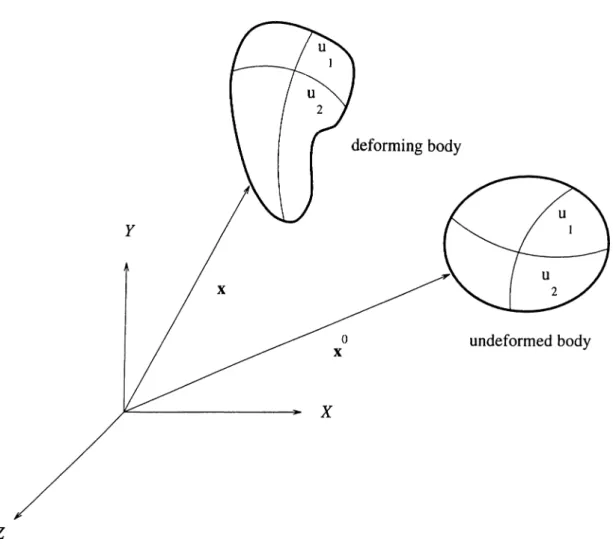
Here, a deformable model is formulated by using the material coordinates of points in the body (denoted by fî). For a solid body u = (ui,?i2,U3) (for a sur­ face u = («1 ,^2) and for a curve u = (^^i)) denotes the material coordinates. The Euclidean 3-space positions of points in the body are given by time-varying vector-valued function x(u, t) = [xi(u ,/), X2(u, i), xs(u, i)]. The body in its nat­ ural rest state is given by x°(u) = [ a ; i ( u ) , . ^ ^ ( u ) ] (Fig. 4.1). The equations of motion for a deformable model can be written in Lagrange’s form as follows (this should hold for all u in the material domain H):

d , d x . d x 6e(x)

(4.1) where yu(u) is the mass density of the body at u, 7 (u) is the damping density of the body at u, f(x, i) is the net externally applied force, and £(x) is the energy functional which measures the net instantaneous potential energy of the elastic deformation of the body.

The shape of a body is determined by the Euclidean distances between nearby points. As the body deforms, these distances change. Let u and u -f du denote the material coordinates of two nearby points in the body. The distance between these points in the deformed body is given by

dl = Gjjdujduj, (4.2)

h3

(4.3) where the symmetric matrix

^ . d x d x

is the metric tensor, which is a measure of deformations. (The dot indicates the scalar product of two vectors.)

CHAPTER 4. NONRIGID MODELS ₁₆

Figure 4.1: Geometric representation of a deformable body for primal formula­ tion.

Two 3D solids have the same shape (differ only by a rigid body motion) if their 3 X 3 metric tensors are identical forms of u = [u\^U2,u^^ for all u in the

material domain fl. Two surfaces have the same shape if their metric tensors G as well as their curvature tensors B are identical forms of u = [^1,^2], for all u in the material domain Ll. The components of the curvature tensor are

d'^x

Bij{x{u)) = n · (4.4)

duiduj ’

where n = [ni,ri2,n3] is the unit surface normal. Two space curves have the same shape if their arc length s(x(u)), curvature k{x{u)), and torsion r(x(u))

CHAPTER 4. NONRIGID MODELS 17

are identical forms of u = [ui]. (See [13] for a detailed discussion of these formu­ lations.)

Using the above differential quantities, potential energies of deformation for use in Lagrange equations can be defined as the norm of the difference between the fundamental forms of the deformed body and those of the undeformed body. This norm measures the amount of deformation away from the natural shape so that the potential energy is zero when the body is in its natural shape and increases as the model gets increasingly deformed away from its natural shape.

If the fundamental forms associated with the natural shape are denoted by the superscript 0, then the strain energy for a curve can be defined as

e(x) = [ w^(s — + w^{k — + w^{t — T°)^du ,

JQ

(4.5) where w^, and xiP are the coefficients for the curve, showing the amount of resistance to stretching, bending, and twisting, respectively. The strain energy for a surface can be defined in a similar way:

Kx) = i_{J Çl} G - G °||L -b ||B - B0||2 (4.6) where the weighted matrix norms || · ||wi and || · ||w2 involve the weighting functions

• ■(ui,U2) and w'fj{ui^U2). Analogously, a strain energy for a deformable solid is yj2du\du2·, llw) and II · I w t '(x) = / ||G — G °\\lfiduidu2du3 Jq (4.7) involves the weighting function tyl (ui, ti2, where the weighted matrix norm || ·

U3)·

These energies denote the amount of energy to restore the deformed objects to their natural shapes. The net external force in Lagrange’s equations is the sum of various types of external forces, such as gravitational force, spring forces, viscous forces, etc.

The weighting functions in the above energies (wjj(ui, U2) and wfj(ui,U2) for

an elastic surface) determine the properties of the simulated deformable mate­ rial. The weighting function wfj(ui,U2) determines surface tensions and sheer

CHAPTER 4. NONRIGID MODELS 18

Gij from its natural coefficients G^j. As wjj is increased, the material becomes

more resistant to length deformation, with w\^ and 1^22 determining this resis­ tance along «1 and «2, and w\2 = determining the resistance to shear defor­ mation. The functions control surface rigidities which act to minimize the deviation of the surface’s actual curvature coefficients Bij from its natural coefficients Bfj. As wfj is increased, the material becomes more resistant to bend­ ing deformation, with wj-i and w^2 determining this resistance along U\ and U2, and WI2 = determining the resistance to twist deformation. To simulate a strechy rubber sheet, for example, we make w]j relatively small and set wfj = 0. To simulate relatively stretch-resistant cloth, we increase the value of lajj. To simulate paper, we make wjj relatively large and we introduce a modest value for

lu'fj. Springy metal can be simulated by increasing the value of wjj [37].

To create animation with deformable models, the differential equations of mo­ tion should be discretized and the system of linked ordinary differential equations obtained from the discretization process should be solved. For the discretization process, there are two basic ways. One way is to choose a finite number of points for a continuous model, and to replace derivatives by differences; this is called the

finite difference method. The other way is to choose a finite number of functions,

and to approximate the exact solution by a combination of those trial functions. If the functions are piecewise polynomials, then the pieces can be chosen to fit the geometry of the problem and a program can generate the polynomials. This method is called the finite element method. It allows a program to assemble the discrete problem and solve it. In our implementation, the finite difference method is chosen for discretization process since difference equations are easier to program and faster to run than a full finite element code.

4 .1 .2

H yb rid F orm ulation

In this formulation, a deformable body is represented as the sum of a reference component r(u , t) and a deformation component e(u, t) (Fig. 4.2). The positions of mass elements in the body relative to a body frame (j) (whose origin coincides

CHAPTER 4. NONRIGID MODELS 19

Deforming body

tion.

with the body’s center of mass and which should be evolved over time according to the rigid body dynamics to have a rigid body motion besides its elastic motion) are given by

q (u ,f) = r(u, ¿) + e (u ,i). (4.8) In this formulation, deformations are measured with respect to the reference shape r. Elastic deformations are represented by an energy e(e) that depends on the position of the reference (body) frame (j). The potential energy functional

CHAPTER 4. NONRIGID MODELS ₂₀

for the hybrid formulation can be written by using simple, linear restoring forces resulting from controlled continuity spline energies [35] as follows:

m=0\j\rzm ---- J'i· (4.9)

where j = ( i i , . . . Jd) is a multi-index with \ j |= ji -|---- -|- jd, and

Qm ^ 9rn

^ du^ . . . d-iPd (4.10)

(d = 1 for curves, d = 2 for surfaces, and d = 3 for solids). The energy density under the integral is a weighted sum of the magnitude of the deformation e and its partial derivatives with respect to material coordinates. The order p of the highest partial derivative included in the sum determines the order of smoothness of the deformation.

The weighting functions Wj(u) in 4.9 control the properties of the deformable model over the body coordinates as in the primal formulation. In the case of sur­ faces (d = 2), the function wqo penalizes the total magnitude of the deformation;

Wio and woi penalize the magnitude of its first partial derivatives; 1020, u>n and W02 penalize the magnitude of its second partial derivatives [38].

4.2

Im p lem en ta tio n o f th e P rim a l F orm ulation

To simulate the dynamics of a deformable surface, we should discretize the follow­ ing expression for the elastic force, which is the approximation of the variational derivative of the expression in 4.6.

e(x) = ^ 9ui d ( d x ' + duiUj A d^x ' duiUj ^ (4.U)

where the functions aij(u,x) and /3ij{u,x) determine the elastic properties of the material. The expressions for Qij{u,x) and /3ij(u,x) are as follows:

CHAPTER 4. NONRIGID MODELS 21

a i j ( w , x ) = wl^{u){Gij - Gl)

Aj(w,x) = wl{u){Bij - B^)

(4.12) (4.13) The discretization is achieved by applying finite difference approximation method.

Since the body coordinates of the models are in the unit square domain, ii = 0 < ui,U2 < 1, we discretize this domain as a regular {M + 1) x (Af + 1) discrete grid of nodes. Here, the inter-node spacings are h\ = 1/M and /i2 = 1/A^ in the «1 and U2 directions, respectively. The nodes on the discrete model are indexed by integers [m,n] where 0 < m < M and 0 < n < Thus, if x (which is a continuous vector function x (u ,t)) is the 3D coordinates of the positions of points, then we discretize it by arrays of continuous time vector-valued nodal variables Xt[m,n] = x { m h i , n h2,t).

Since the elastic force requires the approximations to the first and second derivatives of the nodal variables, we should first define them for the vector­ valued position function X.

The forward difference operators

D f x [ m , n] = (x[m + 1, n] — x[m, n])/hi D2 x[m, n] = (x[m, n -f-1] — x[m, n])/h2

and the backward difference operators

Dj"x[m,n] = (x[m,n] — x[m — l,n ])//ii D^'x[m,n] = (x[m,nj — x[m ,n — l])//i2

can be used to define the forward and backward cross difference operators

Dj'jxfm, n] = D^jx[m, n] = D2 x[m^ n] = (x[m -f- l ,n -f- 1] - x[m -|- l,n ] - x[m ,n -|- 1] -|- x[m, n])/Ai/i2 Z)f2x[m,n] = D^ix[m,n] = Z )fD ^x[m ,n ] = (x[m,nj — x[m ,n — 1] — x[m — l,n ] -|- x[m — l ,n — l])/Ai/i2 (4.14) (4.15) (4.16) (4.17) (4.18) (4.19)

CHAPTER 4. NONRIGID MODELS 22

and the central difference operators

Diix[m,n] = Dj D^x[m,n] = (x[m + l,n ] — 2x[m,n] + x[m — l,n ])//ii (4.20) D22^[i'n,n] = D2 D2X.[m,n] = (x[m ,n + 1] — 2x[m,n] + x[m ,n — l])/hl (4.21)

Now, using the grid functions x[m, n], u;h[m,n], u;? [m,n] to represent their con­ tinuous counterparts, we can discretize 4.12 and 4.13 as follows:

n] = w]j[m, n]{Dfx[m, n] ■ Df x [m , n] — G° [m, n]) (4.22)

bij[m, n] = w^j[m, ra](n[m, n] · DfjX[m, n] - [m, n]), (4.23) where the superscript (+) indicates that the forward cross difference operator is used when i ^ j , and

. i)ji'‘x[m, ra] X D^x[m, n]

^ I Z)/'x[m,n] X i)Jx[m ,n] (4.24) is the surface normal grid function. The elastic force in 4.11 can be approximated as

2

i[m,n]= ^ - D i {aijDfx[m,n]) + Dij{bijDfjx[m,n]). i,j=l

(4.25)

To introduce free boundary conditions on the free edges of a surface, where the inner difference operators in 4.25 attem pt to access nodal variables outside the discrete domain, we set the value of the inner difference operators to zero.

Expressing the grid functions x[m,n] and e[m,n] as x and e in grid vector notation, which denote the 3D positions of model points and elastic force for each model point stored in (M + 1) x {N + 1) vector for an {M + 1) x {N + 1) discrete grid of a deformable model, elastic force can be written in vector form as

i = K (x) . X, (4.26)

where K is an (M + 1)(A^ + 1) x (M + l)(iV + l) matrix. K is a sparse and banded matrix. This becomes a major advantage when we solve the simultaneous system

CHAPTER 4. NONRIGID MODELS ₂₃

Figure 4.3: The band structure of the stiffness matrix K.

of second-order ordinary differential equations. The band structure of K is shown in Fig. 4.3.

Then, we should calculate the total external force for each point of the model. In order to achieve this, we should add the forces effecting a point, which are gravitational, viscous, collision, and constraint forces. The constraint forces are taken into account in the following way. When a constrained point tends to move, an opposite force for bringing it back to its original position is calculated and added to the total external force for that point. Each constrained point has an effect on the total external force for all points in the model depending on the difference between the body coordinates of the points. This coupling effect is taken into account automatically according to the elastic properties of the models. This method for calculating constraint forces gives good results for small time steps. For larger time steps, the model points make small oscillations since this approach corresponds to a corrective action.

The constrained points are specified by the user interactively. The system displays a grid specifying the body coordinates of each point existing in the model to be animated and the user selects the points to be constrained during the animation (that is, the points that will not move during the animation) using mouse buttons (Fig. 4.3). In other words, any point on a model could be constrained to a fixed location in space so that when the model is animated, the constrained points remain in their initial positions. The constraint force that connects a material point uq on a deformable model to a point po in space by a

CHAPTER 4. NONRIGID MODELS ₂₄

D E FO R M A B L E M O D ELİ

Control Points nl : 2 O HSE_0FF

No. planes In x direction : 3 S c a n

2 Curve Points ml : 20 O DEPTH_SORT

No. planes in y direction : 3

Resolution (1-360) : 36

C GOURAUD«SHADE_OFF No. planes in z direction : 3

Figure 4.4: Screen dump during the specification of the parameters for an ani­ mation.

spring IS

f^(u, t) = k{po - x(uo, t))6{u - Uq), (4.27) where k is the spring constant and 8 is the unit delta function.

The forces due to the collision of deformable models with impenetrable ob­ stacles are calculated using the obstacle’s implicit (inside-outside) function. The obstacle exerts a repulsive force on the deformable model which can be calculated as a function of the obstacle’s implicit function such that the force grows quickly if the model attem pts to penetrate the obstacle. This is achieved by creating a potential energy function c exp{f(x)/^) around each obstacle, where / is the

CHAPTER 4. NONRIGID MODELS 25

obstacle’s implicit function, and c and ^ are constants determining the properties of the obstacle. In our system, the user can select different obstacles to exist in an animation sequence by the help of a menu. Ellipsoids, toroids, hyperboloids are possible choices for an obstacle. The repulsive force due to an impenetrable obstacle (expressed using the gradient V of the potential energy function) is f^(u, t) = - c ( ( V / ( x ) /0 e x p ( - / ( x ) / 0 · n) n, (4.28) where n(u, ¿) is the unit surface normal vector of the deformable body’s surface. The implicit functions for different obstacles are given in Appendix A.

The mass density fi{u\,U2) and the damping density 7(^1,«2) are discretized as grid functions and 7[m,n]. Let M be the mass matrix^ an (M +

! ) ( // + !) X (M + 1)(A^ + 1) diagonal matrix with the /i[m,n] variables as diagonal

elements, and C be the damping matrix constructed similarly from 7[m,n]. Then the Lagrange equations can be expressed in grid vector form by the simultaneous system of second-order ordinary differential equations

(4.29) where the net external force on the surface f(ui,U2) has been discretized into the grid vector f which represents the grid function f[m,nj.

We integrate this system through time using a step-by-step procedure. Eval­ uating K (x) at time t + A t and f at t, and substituting the discrete time approx­ imations

^ « (xt+Ai -X t-A i)/2 A i

into 4.29, we obtain the semi-implicit integration procedure A-iX(4.Ai = g^,

where the (M + 1){N -|-1) x {M -|- 1){N + 1) matrix A ,(x,) = K ( x , ) + ( — M + , 2At (4.30) (4.31) (4.32) (4.33)

CHAPTER 4. NONRIGID MODELS ₂₆

and the effective force vector

= it +

with

±t = Ut - Xî-aî)/Aî.

(4.34)

(4.35) Applying the above semi-implicit procedure, we can obtain the dynamic solu­ tion from given initial conditions Xq ^-nd ^ at i = 0. During each time step, we solve the sparse linear algebraic system in 4.32 for the instantaneous configuration

using the preceding solution Xt ^ud [37].

Implementation of the hybrid formulation follows the same steps described for the primal formulation. The elastic force for the hybrid formulation can be written as the variational derivative of the expression in 4.9 as follows:

î(e) - luooe - (u ;io |j) - { w o i § ^ ) + ^ +

(4.36) 9^ (,,, d^e \

duid2 \ duidu2 / + 97f, 92 / „ d^e\

Here, u = (wi,U2) are the surface’s material coordinates.

The only difference between the primal formulation and the hybrid formula­ tion is that the sparse, banded stiffness matrix K is constant in hybrid formula­ tion. The equations of motion can be expressed in semidiscrete form by a system of coupled ordinary differential equations. The system contains two ordinary dif­ ferential equations for the translational and rotational motion of the model as if all of its mass is concentrated at its center of mass, and a system of ordinary differential equations whose size is proportional to the size of the discrete model. These equations are solved in tandem for each time step with respect to the initial conditions given [38].

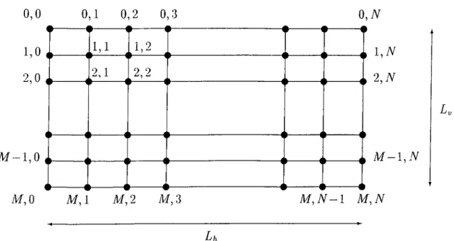
CHAPTER 4. NONRIGID MODELS 27 0,0 1 , 0 2 , 0 M - 1 , 0 0,1 0,2 0,3 · --- #— 1,1 2,1 1,2 2,2 M ,0 M ,1 M ,2 M ,3 Lh 0 , N l,iV 2 , N M - l , N M , N - 1 M , N L.

Figure 4.5: Numbering of the grid.

4.3

Spring Force F orm ulation for D eform ab le

M o d els

In the previous sections, the primal and the hybrid formulations were presented and their implementation details were given. However, the formation of the stiff­ ness matrix automatically is very difficult and sometimes it becomes impossible to solve the differential equations for animating the models because of the nu­ merical ill-conditioning problems. In this section, a new formulation is presented. In this formulation, instead of forming the stiffness matrix automatically, elastic properties are represented as external spring forces. Although handling the elas­ ticities using the stiffness matrix approach is elegant and the most suitable way, our approach is more effective and very fast.

The inter-node spacings on the grid are hi = LhfN, h2 = L y / M in the horizontal and vertical directions, respectively. Initially, we take hi = h2 = h,

CHAPTER 4. NONRIGID MODELS 28

We can apply external forces to many of the grid points at the same time. One type of such external force can be the gravitational force. These external forces are known. Besides, if some of the grid points are constrained to the fixed positions in space, then there will be some unknown spring (constraint) forces at these points.

The line segments in the grid (Fig. 4.5) will correspond to the spring elements. According to the initial positions of the grid points, there will be some spring forces on the model.

The equations of motion for a deformable model (this should hold for all grid points) are

M ^ x + C ^ x + K ( x ) x = f(x)

dt^ dt (4.37)

We can take the elastic force expression as an external force Îk = K ( x ) x , and

take f/c to the right hand side of the equation (4.37). This new form of the equation will simplify the formulation procedure.

The position vector x for the model points is as follows (T denotes the trans­ pose of a matrix):

= [ x j x f ... x j , ] (4.38) where x,· represents all the position vectors of the grid points on the ¿-th row, and

x r = [ x io x i. • • • < « 1

where x*j is the position vector of the grid point {i,j) (*' = 0, 1, · · · , M ; j = 0, i , - - - , i v ) .

In 4.37, M is the mass matrix^ an [M + 1)(A^ + 1) x {M + L){N + 1) diagonal m atrix which contains masses of the grid points as diagonal elements, and C is the damping matrix^ an (M + 1){N -j-1) x {M + 1){N + 1) diagonal matrix which contains dampers of the grid points as diagonal elements.

Note that 4.37 can be rewritten as

CHAPTER 4. NONRIGID MODELS ₂₉

In this way, there will be no need for calculating the entries of the stiffness matrix. Instead of this, it is necessary to find the expressions for the column matrix (external spring forces representing elasticities). The spring force vector can also be partitioned as

f-r _ fT . . . fi 1

Ia' — [Iq II ImJ (4.41)

where the entries in the vector ] correspond to the spring forces acting at the grid points.

Using the discussion in [41] (pp. 359-362), the terminal equation of a two- terminal spring component of free length i in three-dimensional space is given as

fA' = k ( X i - X2 ) - i X l - X 2 (4.42)

Xl - X2II

where Xi and X2 are the position vectors of its terminal points. Note that calcu­ lation of the vector (xi — X2) is essential; it also appears in the second term of this expression. Equation 4.42 can be used to obtain expressions for the entries of fft' in 4.41.

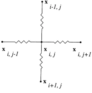
For the grid points not on the boundaries, the elastic force is calculated by adding the spring forces applied to the grid point by its four neighbors.

If i = 1,2,··· , M — 1 and j = 1,2,· fq = ^ ( X i j - X i j - l ) + k [{Xi,j Xi-i,j) + k [ ( X i j - X i j + l ) - ^ ^ + k (Xi,i - X.+1 j) - ^ _-X'+i,h (4.43)

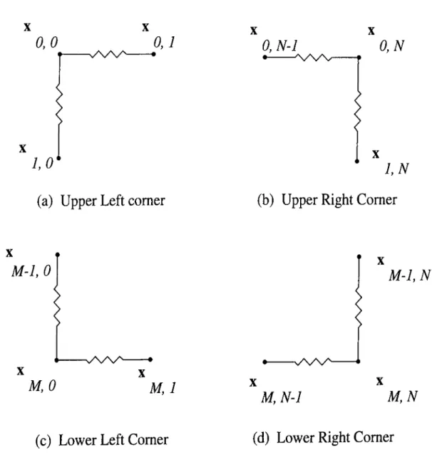
For the grid points on the boundaries, three neighbors have an effect on the elastic force (Fig. 4.7). For the grid points on the corners, only two neighbors have an effect on the elastic force (Fig. 4.8). The elastic force expressions for the grid points on the boundaries and corners are given in Appendix B.

CHAPTER 4. NONRIGID MODELS ₃₀

Figure 4.6: Interactions (couplings) between grid points (general case).

4.3.1

Im p le m e n ta tio n o f th e Spring Force F orm ulation

• Since the initial position vectors of the grid points are known, the vector

Îk can be calculated from the external spring force equations. •

• Then by solving the differential equation in 4.40 at the first step, next values of the position vectors of the grid points are determined.

• The next value of the vector £k is calculated and the process is repeated.

As initial positions, we have h ^ £ in general. Therefore f/i ^ 0. In other words, there will be some internal stresses in the system. U h = £, then = 0. On the other hand, if hi ^ /12, then Îk ^ 0 initially (assuming that all the springs have the same lengths). We may select the lengths of the horizontal springs as li = hi and the lengths of the vertical springs as ^2 = /^2 · In this case, f/v = 0 initially, and some of the £ factors will change to £1 and the remaining ones to £2 in the external spring force equations. Other modifications are also possible; e.g., on the spring coefficients [k).

CHAPTER 4. NONRIGID MODELS 31 - v w ^ OJ -l ■ w v ^ OJ OJ+ l M-IJ I J

(a) Upper Boundary

MJ- 1 ■ v w ^ X X M,j M J+I --- --- · (b) Lower Boundary i-I, 0 _{i-1, N} i, 0 i, 1 ■ w \ ^ i, N-1 i,N i+7, 0 (c) Left Boundary i+1, N (d) Right Boundary

CHAPTER 4. NONRIGID MODELS 32

0 , 0

■ W \ / ^ 0 , 1 0 ,N -1 0 , N

1,0

(a) U pper L eft co m er

1 , N (b) U pper R ight C om er

M-1,0

_M-1,N

M,0

_{M, 1}

_M,N-1

_M,N

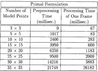
CHAPTER 4. NONRIGID MODELS 33 Primal Formulation Number of Model Points Preprocessing Time (millisec.) Processing Time of One Frame (millisec.) 3 X 3 0 67 5 X 5 1017 ₈₃ 10 X 10 2400 283 15 X 15 3950 600 20 X 20 6250 1183 25 X 25 9500 2000 30 X 30 14216 3883 35 X 35 21749 26182

Table 4.1: Preprocessing and processing times using the primal formulation.

4.4

C om parison o f th e Form ulations

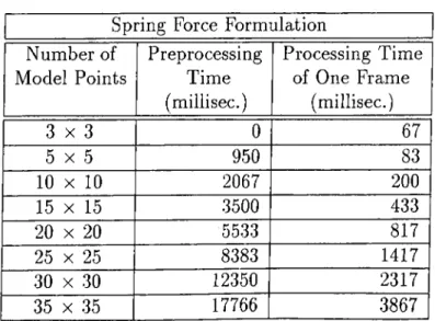
We have compared the processing times for generating an animation frame us­ ing different formulations. To compute processing times, simple Bezier surfaces, having similar elastic properties, are animated using different formulations. Ta­ bles 4.1, 4.2, and 4.3 give the processing times of the animations of the Bezier surfaces of different sizes, for the primal, hybrid, and spring force formulations, respectively. The processing times for each frame given in the tables include

• the time for calculating the external forces for each model point, • the time for calculating the entries of the stiffness matrix*, • the time for calculating the 3D positions of model points, and • wireframe rendering time of the calculated frame.

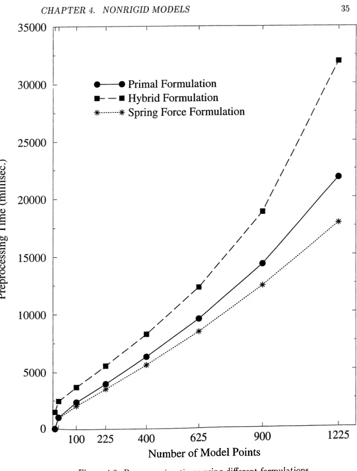
The same information in the tables is also plotted as two graphs (Figs. 4.9, and 4.10) to compare the formulations in terms of the preprocessing times and

‘ This is for the primal formulation; for the hybrid formulation it is included in the prepro­ cessing time. For the spring force formulation stiffness matrix is not formed; external spring forces between model points are calculated for each frame.

CHAPTER 4. NONRIGID MODELS ₃₄ Hybrid Formulation Number of Model Points Preprocessing Time (millisec.) Processing Time of One Frame (millisec.) 3 X 3 1483 67 5 x 5 2483 83 10 X 10 3700 233 15 X 15 5500 400 20 X 20 8200 650 25 X 25 12233 1050 30 X 30 18749 2017 35 X 35 31932 20166

Table 4.2: Preprocessing and processing times using the hybrid formulation.

Spring Force Formulation Number of Model Points Preprocessing Time (millisec.) Processing Time of One Frame (millisec.) 3 x 3 0 67 5 x 5 950 83 10 X 10 2067 200 15 X 15 3500 433 20 X 20 5533 817 25 X 25 8383 1417 30 X 30 12350 2317 35 X 35 17766 3867

Number of Model Points

CHAPTER 4. NONRIGID MODELS ₃₇

processing times. Although it seems from the graphs that the hybrid formula­ tion is superior to the primal formulation, they are complementing each other for different elasticity properties. The nonquadric energy functional in primal formulation causes a nonlinear elastic force associated with the deformable body to appear in the partial differential equations of motion. Nonlinearity results because the elastic force attem pts to restore the shape of the deformed body to a rest shape. The advantage of nonlinear elasticity is that it is in principle the most accurate way to characterize the behavior of certain elastic phenomena. How­ ever, it can lead to serious practical difficulties in the numerical implementation of deformable models for animation. The hybrid formulation offers a practical ad­ vantage for fairly rigid models, whereas primal formulation becomes unpractical due to the nonquadric energy functional with increasing rigidity and complexity of the models.

The spring force formulation generates animation frames faster than the pri­ mal formulation. The hybrid formulation is superior to the spring force formu­ lation for models having small size (less than 1000 model points). For larger models, spring force formulation is faster. The primal formulation is the most suitable formulation for highly rigid models. However, it is very difficult to form the stiffness matrix automatically. Spring force formulation bypasses this problem by modeling elasticities using external spring forces between model points.

An important advantage of the primal formulation over other formulations is that it is easier to establish an intuitive link between the weighting functions of the deformable models and the resulting elastic behavior. This is due to the nature of the weighting functions as explained in section 4.1.

4.5

O ther M eth o d s for th e A n im a tio n o f N on-

rigid M od els

The formulations that we have used employ continuous elasticity theory to model the shapes and motions of deformable models. There are other approaches to