Л 2 ^ Á THES2S Уг ЗП-,.К,^::МТ * ■,i . ;іц J** A ·*'*<·* " T *» w .“!" *' 7 'V />:!'■'■■.,; ,.í -i»? ¡r. ’ÍS. , ; I .tf·. 5'· w W ·,Α/’ 4*)/
MODELING THE SOFTWARE FAILURE PROCESS
AND SOFTWARE RELIABILITY
A T H E S I S S U B M I T T E D T O T H E D E P A R T M E N T O F I N D U S T R I A L E N G I N E E R I N G A N D T H E I N S T I T U T E O F E N G I N E E R I N G A N D S C I E N C E O F B I L K E N T U N I V E R S I T Y IN P A R T I A L F U L F I L L M E N T O F T H E R E Q U I R E M E N T S F O R T H E D E G R E E O F M A S T E R O F S C I E N C E
By
Sava§ Dayanik
September, 1996
іЗЗб
SJ35239
11
I certify that I have read this thesis and that in rriy opinion it is fully adequate, in scope and in quality, as <f. t]|Les^^^r the degree of Miister of Science.
Asso\^^'oV. Üllicü (pirler (Advisor)
I certify that I have read this thesis and that in my opinion it is fully adequate, in scope and in quality, as a thesis for the degree of Master of Science.
Prof. Halim Doğrusöz
I certify that I have read this thesis and that in my opinion it is fully adequate, in scope and in quality, as a thesis for the degree of Master of Science.
^ ________________
soc. Prof. Y. Yasemin Serin
Approved for the Institute of Engineering and Sciences;
Prof. Mehrnet Bai^
A B S T R A C T
MODELING THE SOFTWARE FAILURE PROCESS AND
SOFTWARE RELIABILITY
Savaş Dayanik
M.S. in Industrial Engineering Supervisor: Assoc. Prof. Ülkü Gürler
September, 1996
Бог the last few deccides, the computer systems have replaced the man power in many important areas of life. Financial markets, production and service systems are controlled either fully by the computers or by the managers who extensively use the computers. Therefore, a major failure of a computerized system iriciy end up with a catastrophe that may affect a hirge number of people adversely, fo r this reason, reliability of computer systems attracts tlie attention of the researchers and practitioners.
Software is one of the major component of a computer system. Therefore, in this thesis, we study the stochastic nature of the failure process of a software during the debugging phase. We propose a mathematical model for the software fciilure process which may also lead to prediction of future reliability. Different from many other available software relicibility models, we particularly try to incorporate the structural properties of a softwcire such as the number ol its different instruction paths cuid their logical complexities. The debugging phase is assumed to be composed of successive test sessions. Distribution functions of the length of a test session and the remaining number ol faults cifter a test session are computed. A stopping condition lor the debugging phase is proposed.
Keywords: Software Reliability, Software faults, Markov Renewal Processes, Spatial Poisson Processes.
I V
ÖZET
BİLGİSAYAR BOZULMA SÜRECİNİN VE BİLGİSAYAR
YAZILIM GÜVENİLİRLİĞİNİN MODELLENMESİ
Savaş Dayarnk
Endüstri Mühendisliği, Yüksek Lisans Tez Yöneticisi: Doç. Dr. Ülkü Gürler
Eylül, 1996
Son yıllarda, bilgisayarlı sistemler yaşamımızdaki bir çok önemli alanda in san işgücünün yerini cddılar. Finans piyasaları, üretim ve servis sistemleri ya tamamen bilgisayarlar ya da yoğun olarak bilgisayarları kullanan yöneticiler tarafından kontrol ediliyorlar. Bu yüzden, bir bilgisaycir sisteminin bozulması, bir çok insanı kötü etkileyebilecek bir felaketle sonuçlcuıabilir. Bu sebeble, bil gisayar sistemlerinin güvenilirliği, araştırmacıların ve uygulayıcıların dikkatini çekmiştir.
Yazılım bir bilgisayar sisteminin önemli parçalarmdandır. Bu yüzden, bu tezde, yazılımın bozulma süreci için bir mcitematiksel model önerdik. Varolan birçok yazılım güvenilirlik modellerinden farklı olarak, yazılımın güvenilirliğini daha doğru tahmin edebilmek için, özellikle, farklı komut dizgelerinin sayısı ve karmaşıklıkları gibi bir yazılımın yapısal özelliklerini modelimizde kullandık. Hatalardan ayrıştırma sürecinin birbirini takip eden sınama oturumlarından oluştuğu varsayıldı. Sınama oturumlarının uzunluğunun ve her sınama oturu mundan sonra kalan hataların sayısının dağılım işlevleri bulunmuştur. Hatci- lardcui ayrıştırma süreci için bir durma koşulu önerilmiştir.
Anahtar Sözcükler: Yazılım Güvenilirliği, Yazılım Hataları, Markov Ye nilenme Süreçleri, Uzamscd Poisson Süreçleri.
I would like to express my gratitude to Assoc. Prof. Ülkü Gürler due to her supervision, suggestions, and understanding to bring this thesis to an end.
I am especially indebted to Prof. İzzet Şahin for his invaluable guidance, encouragement and above all, for the enthusiasm which he inspired on me throughout this study.
I am also indebted to Prof. Erhan Çndar, John Musa and Prof. Mehmet Şahinoğlu lor the discussions on the various aspects of softwcire reliability the- ory.
I would like to thardi to Prof. Halim Doğrusöz and Assoc. Prof. Yasemin Serin for showing keen interest to the subject matter and accepting to read and review this thesis.
1 cannot fully express rriy gratitude and thanks to Aynur Akkuş and my parents for their morede support and encouragement.
1 would also like to thank to Abdullah Çöndekçi, Abdullah Daşcı and Mustcvfa Karakul for their friendship and support.
Contents
1 Introduction and Literature Review 1
1.1 Literature R e v ie w ... 7 1.1.1 Black-Box M od els... 7 1.1.2 Software Reliability Models Incorporating Logical Struc
ture of the Software... 14
1.1.3 Unification of Existing Software Reliability Models 16
1.1.4 Further Topics in Software Reliability Literature... 19 1.2 Scope and Outline of the S t u d y ... 20
2 A Conceptual M odel of Software Failure Process and Prelim
inaries 22
2.1 Preliminaries 23
2.1.1 Basic Concepts in the Software Reliability Theory . . . . 24 2.1.2 Littlewood’s Conceptual M o d e l ... 27
2.2 A Preliminary Mathematical Model for the Software Reliability 31
2.3 An Alternative Approach to Model the Software Reliability . . . 36
2.4 Illustration of the Key Concepts in the Model on a Sample Software 43 2.4.1 Overview of the Sample P r o g r a m ... 44
2.4.2 Sample Runs of the Program 46
2.4.3 Preliminaries for Reliability Model Construction of the
Sample Pi'ogram 48
2.4.4 Some Concluding R em arks... 57
3 Mathematical M odel of Software Failure Process and Software
Reliability 58
3.1 Marginal Contribution of a Software Failure to the Software Re
liability 59
3.1.1 Probability Distribution of the Number of Fault Sets that
Cover a Given Input S t a t e ... 60 3.1.2 Extension of the Model constructed on 77 to a Model in
7 7 ^ ... 73
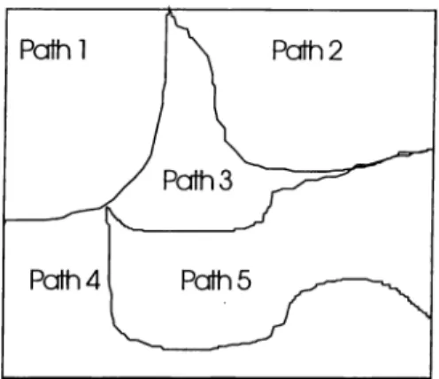
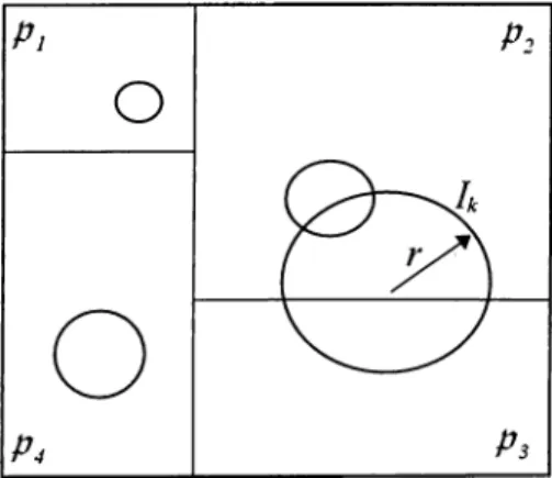
3.2 Arrangement of Path Sets in the Input Space 76
Dffending Command = 7
Error = nametype : syntaxerror
Stack =
2017
2039
24
1 Introduction and Literature Review 1
1.1 Literature R e v ie w ... 7
1.1.1 Black-Box M od els... 7
1.1.2 Software Reliability Models Incorporating Logical Struc ture of the Software... 14
1.1.3 Unification of Existing Software Reliability Models 16
1.1.4 Further Topics in Software Reliability Literature... 19 1.2 Scope and Outline of the S t u d y ... 20
2 A Conceptual M odel of Software Failure Process and Prelim
inaries 22
2.1 Preliminaries 23
2.1.1 Basic Concepts in the Software Reliability Theory . . . . 24 2.1.2 Littlewood’s Conceptual M o d e l ... 27
2.2 A Preliminary Mathematical Model for the Software Reliability 31
2.3 An Alternative Approach to Model the Software Reliability . . . 36
CONTENTS vu
2.4 Illustration of the Key Concepts in the Model on a Sample Software 43 2.4.1 Overview of the Sample P r o g r a m ... 44
2.4.2 Sample Runs of the Program 46
2.4.3 Preliminaries for Reliability Model Construction of the
Sample Program 48
2.4.4 Some Concluding R em arks... 57
3 Mathematical M odel of Software Failure Process and Software
Reliability 58
3.1 Marginal Contribution of a Software Failure to the Software Re
liability 59
3.1.1 Probability Distribution of the Number of Fault Sets that
Cover a Given Input S t a t e ... 60 3.1.2 Extension of the Model constructed on 77 to a Model in
7 7 ^ ... 73
3.2 Arrangement of Path Sets in the Input Space 76
3.3 The Mathematical Model of the Software Reliability 79
3.3.1 The Description of the Debugging P h a s e ... 81 3.3.2 The Mathematical Model for Evolving Software Reliability 83 3.3.3 A Stopping Time for the Debugging P h a s e ... 92
1.1 Hardwai'e and Software Cost Trends... 2
1.2 Failure Rate of a Typical H ardw are... 5
1.3 Failure Rate of a Typical Software... 5
1.4 Research Agenda in Software Reliability 13 2.1 A Conceptual Model of the Software Failure P rocess... 28
2.2 Realisation of the i-th Debugging C y c le ... 35
2.3 The Fault Sets after the i-th Debugging C y c l e ... 36
2.4 Partition of Input Space into Path S e t s ... 38
2.5 Step 2 and 3: Path Sets and Fault Sets (L = 4, M = 4 ) ... 40
2.6 i-th Debugging Cycle Stops with a Softrvare F a ilu r e ... 41
2.7 The Fault is Removed before the (i-l-l)st Debugging Cycle Starts 42 2.8 Flow Chart of the Program 47 3.1 Sketch o f p ( r ) ... 64
3.2 Approximation of p(r) 67
LIST OF FIGURES IX
3.3 Maximum Likelihood Estimation of yU... 71
3.4 A Sample Input State 81
3.5 The Debugging Phase of a S oftw are... 84 3.6 Evolution o f Debugging P h a s e ... 85 3.7 Debugging Phase with Constant and Equal Execution Times . . 86
2.1 The Path Sets of the P ro g ra m ... 50 2.2 Examples for Fault Sets of the Program ... 54
3.1 Likelihood Estimates of /r 70
3.2 Comparison of Estimators of ... 73 3.3 List of Path Sets of the Sample Program in the Order of Com
plexity ... 78 3.4 Arrangement of the Path Sets of the Sample P ro g ra m ... 79
Chapter 1
Introduction and Literature
Review
Nowadays, computers are extensively used in numerous areas: They control expensive machines in the manufacturing systems, continuously check and reg ulate vital parameters in the nuclear power stations, maintain many commu nication networks, control traffic flow in the airport and in the cities, keep and process enormous amount of data in financial markets, etc. Therefore, malfunction of computer systems can result in disasters. This fact leads the researchers to study the methods to measure reliability of the computer sys tems. Unfortunately, classical reliability theory is not sufficient to model the reliability of such systems.
Computer systems are composed of two major parts: Hardware and Soft
ware. Hardware systems are subject to aging. Therefore, the classical reliability
theory can be applied to them. However, unlike hardware systems, software systems are not subject to physical stress and fatigue. They stay as good as new regardless o f how old they are. On the other hand, softwares are still opt to fail like hardwares, but the characteristics of software failure process is different from those of hardware failure process.
100
1955 Year 1985
Figure 1.1: Hardware and Software Cost Trends
it is important to study software reliability along with hardware reliability. Shooman [32] figures out the shares of hardware and software in computer system development costs between the years 1955 and 1985 (see Figure 1.1).
Hardware systems become cheaper due to technological advances in inte grated circuit technology. But, cost of developing a software increases:
The basic problem in the software area is that the complexity of tasks which software must perform has grown faster than the tech nology for designing, testing and managing software development. Furthermore, software costs are primarily labor intensive, rather than technologically dependent, and man-hours spent on software development are roughly proportional to the size of the program measured in lines of code... Thus, a software complexity has in creased over the years, the man-hours for a typical project have increased, as have labor costs due to inflation. By contrast, the advances in integrated circuit technology have resulted in a relative decrease in hardware costs. The net result is that an increasingly larger portion of computer system development costs are due to software...
C H A P T E R 1. IN T R O D U C T IO N A N D L IT E R A T U R E R E V IE W
For a product which requii'es large volume production, the im pact of development costs on the per unit production cost can be small. The manufacturing cost of hardware includes parts, assem bly, inspection and test. The manufacturing cost of software in cludes the small cost of storage media (disks or tapes), the operator and computer time cost of copying the master version of the pro gram and the cost o f printing extx'a copies of the pertinent operating manuals... [32]
Thus, to reduce the contribution of software development in the cost of the entire computer system, computer scientists develop various software design and testing methods. At this point, a quantitative measuring tool is required to compare the performances o f alternative methodologies. Software reliability metrics can help the developers not only to produce a high-quality product but evaluate the effectiveness and efficiency of software engineering processes. Musa discusses three aspects of this in [19], [21], [23], and [22] to some extent:
1- Software reliability figures can be used to evaluate software engineering technology...
2- A software reliability metric offers the possibility o f evaluating status during the test phases of a project.
3- Software reliability can be used as a means for monitoring the operational performance of software and controlling changes to the software.
The comments o f Shooman and Musa clarify the necessity to explore soft ware reliability measurement tools.
The difference between the hardware and software failure processes is very sharp. Musa [23] points out the difference between hardware and software failure processes:
The concept of software reliability differs from that of hardware reliability in that failure is not due to a wearing-out process. Once
a software defect is properly fixed, it is in general fixed for all time. Failure usually occurs only when a program is exposed to an envi ronment that it was not designed or tested for. The large number of possible states of a program and its inputs make perfect com prehension of the program recpiirements and implementation and complete testing of the program generally impossible. Thus, soft ware reliability is essentially a measure of confidence we have in the design and its ability to function properly in all environments it is expected to be subjected to. In the life cycle of software there are generally one or more test phases during which reliability im proves as errors are identified and corrected, typically followed by a non-growth operational phase during which further corrections are not made (for practical and economical reasons) and reliability is constant.
Hardware reliability studies are mainly concerned with physical deteriora tion of hardware whereas software reliability studies concentrate on the design problems. We may even call the software reliability as design 7'eliability. One may think that design reliability concept can also be applied to hardware man ufacturing processes. But, ‘ because o f the probability o f failu7'e due to wear
a,7i.d other physical causes has usually bee7i 7nuch greater than the probability of failu7’e due to an u7irecog7iized design problem hardware reliability models opt
to ignore the impact of the design failure process on the overall reliability of hardware (Musa [22]).
Comparison of the failure rates of a typical hardware and software summa rizes what we talk about the differences between the hardware and software failure processes.
Graph of a typical failure rate function of a hardware is like a bathtub as seen in the Figure 1.2. In the early failure period (usually called infant- mortality or burn-in period), inoperable or incompatible parts of hardware may cause the system to fail. As they are replaced, the hardware is adapted to the environment and failure rate is decreased. In the normal operating
C H A P T E R 1. IN T R O D U C T IO N A N D L IT E R A T U R E R E V IE W
Figure 1.2: Failure Rate of a Typical Hardware
period, the hardware is pretty resistant to the environment. Therefore, the failure rate is fairly constant. After a while, fatigues increase and hardware cannot compensate the physical stress of environment. Eventually, a wearing- out period follows the normal operating period, and, failures occur more often. Therefore, hardware becomes more and more unreliable.
Operational Phase
Figure 1.3: Failure Rate of a Typical Software
On the other hand, failure rate of a typical software has a tendency to decrease. Figure 1.3 is an approximate sketch of failure rate function of a
software. It should be mentioned that there is not a single shape for the failure rate function of a software on which the researchers agree and Figure 1.3 is illustrated for the sake of simplicity.
The points A, B, C, D and E are the times when a software failure occurs. At those points, the software failure rate changes because some faults in the software are fixed. It is customary to assume that the time needed to fix faults and remove them is negligible. Therefore, jumps occur at those points. Failure rate decreases and software reliability increases when the fault is successfully fixed and removed (points A, B, D, E). But, sometimes, as the fault is removed, debugging team may introduce new faults into the code which causes the failure rate to increase (point C). After the debugging phase is stopped and software is released to the market, no more fault is removed and failure rate does not change.
The other main difference between software and hardware failure process lies in the ability of the corresponding production systems to replicate a typical product. In hardware manufacturing systems, factors such as tool wearing, experience of labors working in different shifts, materials coming from different suppliei's, etc. make it difficult to produce products in a mass with a desired reliability. Therefore, various quality control activities are undertaken. On the other hand, the replication of a software is trivial and all replicated softwares have exactly the same characteristics including the reliability.
Despite the differences between the software and hardware failure processes, software reliability theory should be compatible with hardware reliability the ory. This is necessary because, practically, the main concern is the reliability of the whole computerized systems. Therefore, many concepts and notions of hardware reliability theory such as failure rate, mean time to failure (M TTF), etc. are also adapted to software reliability theory. By the same reason, the definition of software reliability is very similar to the hardware reliability: Soft ware reliability is defined by Musa [26] as the probability o f failure-free executiov·
o f a computer program in a specified environment fo r a specified time.
C H A P T E R 1. IN T R O D U C T IO N A N D L IT E R A T U R E R E V IE W
related to the software reliability theory in the past. Thereafter, we give a short outline of the remaining part of this study.
1.1
Literature Review
Software Reliability Modeling studies started in the late 60’s. But, research was accelerated in 70’s. In this section, we review some of the software reliability models more closely to give an idea about how the software reliability modeling practice is evolved^. Our main point in this study will be to find ways to benefit from the structural information of the software to get more accurate and robust estimates of its reliability. Therefore, we primarily divide the software reliability literature into two main parts: Models of black-box approach and models incorporating the logical structure of software. We present examples of those two classes in separate subsections.
1.1.1
Black-Box Models
Researchers using black-box approach mainly concentrate in the data collected on time between successive failures and number of faults in the program. They try to investigate which probability distribution represents the data best. Log ical structure of the program and physics of the programming environment have not been much considered in those models. Therefore, they are easy to understand and apply. Because the data requirements are small, application of black-box models is cheaper than their counterparts.
One of the earliest model in this class is Jelinski-Momnda Reliability Model. The main assumptions are
1- The rate (of detection of software errors [^]) is proportional
^The reader may first want to refer to Subsection 2.1.1 for the definitions of some funda mental concepts that are frequently used in this section.
at any time to the current error content in the software package. Between error detections, the rate is constant.
2- All remnant errors are equally likely to occur, and the time separations between the errors are statistically-independent.
3- Errors which are detected are instantly and perfectly cor rected without introducing any new errors...[18].
Failure rate of the software between two successive failures is constant. The inter-failure times are assumed to be exponentially distributed independent random variables. But, they are not identical because rate of inter-arrival times are assumed to change as faults in the software are fixed. Authors computed M T T F and reliability of software at any time.
All three assumptions of Jelinski-Moranda Model are heavily criticized. Goel and Okumoto [6] proposed that independence of inter-failure times is unrealistic. In their Model (Goel-Okumoto Model), they assumed that time between k-th and (k l)-st failures is dependent on the time to A;-th failure. Different from Jelinski-Moranda model, number of faults in the program before debugging is a random variable. They modeled the fault-counting process with a non-homogeneous Poisson process. They formulated various rate functions for this process and explored reliability function.
Later, some other software reliability models based on non-homogeneous Poisson process are developed by fitting various functions for the mean-value of the process [27], [40], [41].
In the mean time, Musa [19] proposed his Execution Time Model. In his paper, he claimed that Moranda’s assumptions are valid if the failure times are measured in terms of processor time, so called execution time. In particular, he reported that times between successive failures measured in terms of execution time are exponentially distributed. Unlike Jelinski-Moranda model, he treats the number of corrected errors in the software as a continuous random variable. His major contribution is introduction of execution time concept. Besides this, he developed a calendar time component of his model which actually projects
C H A P T E R 1. IN T R O D U C T IO N A N D L IT E R A T U R E R E V IE W
the measures in terms of the execution time on the calendar time. By doing this, he combined the capacity problems resulting from the constraints on man power and available computational time with the software failure process in theory. Thus, resources can be used effectively and efficiently to improve the software up to a satisfactory level of reliability at a reasonable cost within a permissible time interval. Moreover, the software reliability activities can be measured in terms of monetary terms.
In his following paper, Musa [21] makes the foundations of his execution time model rigid. He published the statistical evidence for the typical assump tions which are also adopted by many other softwai'e reliability models. He claims that the statistical analyses indicate that
1- failure intervals are independent of each other,
2- the execution times between failures are piecewise exponen tially distributed,
3- the failure (hazard) rate is proportional to the expected num ber of remaining faults.
This paper together with [20] is invaluable for the software reliability studies because, even today, we do not have enough data on failure processes o f real-life software projects.
Musa tested his Execution Time Model on various data sets, and issued some useful methodologies for software engineers to apply the model to real- life projects [23].
In the effect of Bayesian approach to the software failures, Musa [26] mod ified Execution Time Model into Logarithmic Poisson Execution Time Model. In his new model, he assumes that rate of inter-failure times is not a linear but an exponential function of number of remaining faults in the software. He shows that Logarithmic Poisson Execution Time model performs better than the Execution Time Model.
...reductions in failure rate resulting from repair action following eaiiy failui'es are often greater because they tend to be the most frecpiently occurring ones, and this property has been incorporated in the model.
Littlewood is one of the pioneers in the software reliability theory who discussed most of the software modeling practice in his early papers. Here, I will go over four of those papers.
Littlewood ([12], [14], [16], [17]) concentrates on the main assumptions of existing models and performance measures used to quantify the reliability of a software. Almost all software reliability models assume that
A .l. failure rate of software at any time is proportional to the number of remaining (physical) faults and it is constant between successive times of fault-fixing,
A .2. every time a failure occurs the related faults are successfully fixed and removed for certain,
A.3. removal of every fault improves failure rate of software in the same amount,
A .4. Mean time between failures (MTBF) is widely used to measure how reliable a software is, and, to predict its reliability in the future.
Littlewood attacks those four main assumptions in his papers. But, what makes those papers original is the introduction of a conceptual model of soft ware failure process.
Littlewood emphasized the importance of proper definition of the problem we attempt to solve. If a problem is carelessly defined, our studies may end up with a right solution to the wrong problem.
What is our problem? We want to set up a metric and some tools to evaluate
the reliability o f a software in terms o f users ’ specifications. We expect that
C J IA P T E R 1. IN T R O D U C T IO N A N D L IT E R A T U R E R E V IE W 11
actions to improve customer satisfaction. This fact needs to be emphasized because, as Musa stated in one of his papers, software developers and code writers are opt to fix all the faults in a code. They believe that a software product is unreliable as long as it contains undiscovered faults. Most of the reliability models implicitly adopted this point of view. Assumptions similar to A .l refers to this belief. But, a user does not care about how many faults there are in a software. If he never experienced any of those faults, he would appreciate the software as 100 per cent reliable. Furthermore, not all faults are experienced by a user with equal frequency. A pi'ogram with two faults agitated infrequently will be considered more reliable than another with only one fault agitated more often.
Littlewood distinguishes different assessment of software reliability by users and code developers by calling the first one as operational reliability. He puts the problem in its proper place: We should develop tools to evaluate operational reliability o f a software.
In the mean time, he reveals the connection between operational reliability and total number of remaining faults in the code. But, he criticizes existing models because they oversimplify that connection by assuming that faihuvs rate is proportional to the number of remaining faults in the code.
In short, he blames those models because they solve the wrong problem. Second issue Littlewood addresses is unconscious usage of M TBF for soft ware failures. He warns researchers when they draw analogies between hard ware reliability and software reliability. He emphasizes the fact that hardware decays due to aging. Therefore, it is natural to model the lifetime of the com ponents o f a hardware system with a distribution having finite moments. On the other hand, software are not subject to environmental (physical) stress. Therefore, once a software is upgraded, it performs well at any time no matter how much time has passed since the last upgrade. Littlewood calls this prop erty of software product as reliability growth. Littlewood also argues that it is not exceptional to have completely fault-free software. He bases this conclu sion on widely used programming techniques such as top-down modular design:
Programs are usually composed of relatively small modules and fixing all faults in them is practically possible. This may result in a fault-free software as a whole.
Thus, time-between-software-failures could have momentless probability disti’ibution. Therefore, M TBF can increase to infinity, and any estimate based on finite-valued samples of observed time-between-failures is meaningless.
Instead of using MTBF, Littlewood proposes to investigate distribution function of time-to-failure. Even, the quantiles of its distribution function is more informative than MTBF. Another side-effect of M TBF is that it does not give any idea about the variability of time-between-failures.
Author’s caution about reliability growth should invite us to be careful when we use renewal-theory-based techniques to attack the problem. Little- wood suggests that failures -renewals in some generalized meaning- should not occur after some finite period. Then, renewals are transient. Therefore, powerful tools coming from studies on persistent renewal processes are no more remedy. Especially, nice results about availability discovered for hardware case are helpless when we deal with software reliability.
Third issue Littlewood draws our attention to is the individual contribution of each fixed fault to the improvement of software reliability. It is not sensible that removal of every fault improves the failure rate in the same amount as many popular models assume. Some faults are frequently agitated than the others. Therefore, they cause certain failures to appear frequently. So, we may conclude that failures with high occurrence rate affect the reliability o f the whole software system more adversely than the others. But, those failures with high occurrence rates are more likely to be fixed earlier than their counterparts. Therefore, we can conclude that fixing earlier failures improves the reliability o f the software more than the later failures. That is, diminishing returns of fixing marginal failures -law- is in act. Here, Littlewood assumes that the debugging process is perfect for the sake o f simplicity. But, he also takes into account the imperfect fault-fixing operations once he introduces his conceptual model.
C H A P T E R 1. IN T R O D U C T IO N A N D L IT E R A T U R E R E V IE W 13
It is A.3 that Littlewood may have most elaborately worked out. This is one of the key item of his conceptual model. We will present his approach to this problem, together with the conceptual model he proposed later in the second chapter. As I mentioned earlier, his conceptual model is our starting point in this study.
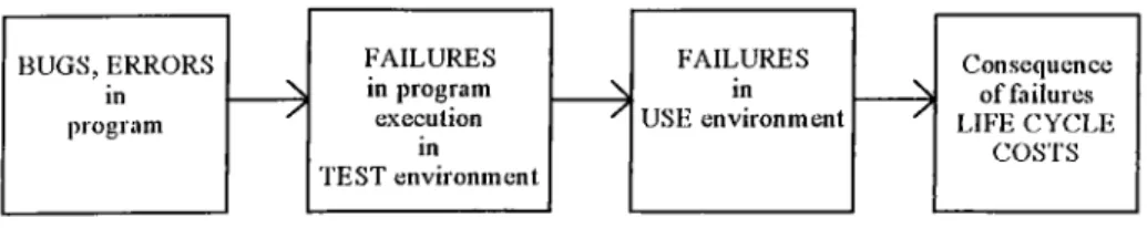
Littlewood also warns the researchers about not to lose the main point in the software reliability modeling studies. He sketches the mission of the software reliability studies with a simple figure (see Figure 1.4). The point we should arrive is the well developed theory that explores the consequence of failures in monetary terms. He summarizes the past and the future of software reliability studies in four stages. So far, the first two stages are vigorously studied although, he thinks, there are many misleading conceptualisations of many notions. But, last two stages are still not explored thoroughly [16].
BU G S, ERRORS FA ILU RES FA ILU RES Consequence
in \ in program \ in \ of failures
program y execution y USE environment y LIFE C Y CLE
in CO STS
T E ST environment
Figure 1.4: Research Agenda in Software Reliability
One o f the interesting model is constructed by Kremer [9]. Kremer models the software failure process with a birth and death p7vcess. A birth represents a fault spawned by the debugging team after an unsuccessful fault-fixing attempt. A death represents a successful fault-correction. It is also allowed that the fault-content of the software may not change after a fault-fixing attempt.
Before concluding the review of black-box models, I should reveal that a vast number of software reliability models are also developed by Bayesian
School [3], [4], [10], [11], [34], [33], [35]. They are usually based on Time-Series
1.1.2
Software Reliability Models Incorporating Logical
Structure of the Software
Besides black-box modeling practice, there are some other approaches that make use of some inhei'ent characteristics of the software in order to measure its reliability accurately.
One of them is fault seeking. This is actually a very popular statistical method used by zoologists to estimate the size of wild animal populations. An example is the estimation of number of fish in a pond. As a first step, researchers catch a number of fish from the pond, mark each of them with a sign and leave them back to the pond. Next, they catch a sample of fish from the pond and count the marked fish in the sample. The basic assumption is that the fish population in the pond does not change during the time interval passed between marking the fish and taking the sample. Then, the number of marked fish in the sample has a Hypergeometric distribution. The only unknown parameter is the size of the fish population. By using maximum likelihood estimation technique, the size of fish population is estimated.
The same method is applied to the software. Some faults are spawned into the code of software on purpose by the programmers who have the similar background and experience as the code developers of the software have. During the debugging phase, the spawned and inherent faults which are fixed by the testing team are counted. Here, the spawned faults are analogies of marked fish in our example. Thus, the total number of inherent faults in the software is estimated by using maximum likelihood approach. This estimate is used to compute pointwise availability of the software. Some of well known fault seeking models are developed by Miller, Lipow and Basin [5], [31].
There are major criticisms addressed to the fault seeking method. First and the most important one is that it causes the limited man-power and com putational time to be wasted to fix the spawned faults. Second criticism is related to the representativeness of spawned faults for the inherent faults. The inherited faults are, usually, more difficult to be fixed than the spawned faults.
C H A l^ T E R 1. IN T R O D U C T IO N A N D L IT E R A T U R E R E V IE W 15
Therefore, probability of detection of the spawned and inherent faults are not equal. This is contrary to the basic assumption behind the claim that the number of spawned faults fixed during the debugging phase has a Negative Binomial distribution.
Another modeling approach, Input-Domain based Modeling, makes use of the input space of a software to estimate the software reliability. The main idea underlying those models is to make inference about the behavior of the software in the future by observing its response to a sample of input states which is far smaller than the input space.
Nelson Model is one of the earliest Input Domain Based Models [5]. In
this model, n input states are randomly selected from the input space and the software is exercised with each of those n inputs. Number of runs that result in an unsatisfactory output, say n^., is counted. Then the reliability of the software is computed as 1 — n,f,/n.
One of the draw-backs of Nelson Model is the assumption that every input state is randomly chosen. Researchers argue that the randomly chosen sample of input states may not be representative for the input space as a whole. Brown, Lipow and Ramamoorthy [29], develop new models to overcome this difficulty in the Nelson Model.
The last example for the modeling approaches which make use of inherent features o f a software to model its reliability is Markovian models.
In 1975, Littlewood proposed his first Markovian Model [13]. In his paper, Littlewood assumes that the software is composed of many small subroutines. Subroutines are elementary sub-units which are designed to perform several stages of the function of the whole software. Because the tasks performed by a subroutine are usually simple, they are easy to develop and test.
In his model, Littlewood studies two different kinds of failures. First one is the failure o f a subroutine. It occurs when a subroutine does not perform the task which it was designed for. Second type failure may occur during the switch
between two subroutines. Switching failures occur especially when a subroutine passes an inappropriate parameter type or value to the next subroutine.
Littlewood assumes that every subroutine has its own continuous time fail ure process. The failure processes of different subroutines are independent from each other. In his paper, he particularly substitute a Poisson process for each failure process within every subroutine. The rates of Poisson processes for different subi'outines are allowed to be different.
Switches between successive subroutines are ruled by a continuous time Markov process. For every pair o f subroutines he defines a Bernoulli process. The switch from one subroutine to the other may be successful with some constant probability between 0 and 1 which is uniquely determined by the calling and called subroutines, or, may cause the software to fail. He gives some asymptotic results on the reliability function of the software.
In his later paper [15], Littlewood extends his previous Markovian Model by modeling the switches between successive subroutines with a semi_Markov process.
In a recent study [38], Whittaker and Thomason assumed that the input states chosen by a user follows a Markov property and they studied the ways to design the best testing strategies.
In the next section, we shall mention about a new trend in the software reliability studies.
1.1.3
Unification of Existing Software Reliability M od
els
As it can be observed from the previous discussion there is a vast literature on software reliability models. Xie [39] overview only 100 of them in his review paper. However, there does not exist a unique model which beats others in every aspect.
C H A P T E R 1. IN T R O D U C T IO N A N D L IT E R A T U R E R E V IE W 17
This creates an overwhelming problem for the practitioners. Engineers par ticipated in a softwax'e development project cannot decide on which reliability model best suits their software project in the plethora of models. Therefore, contemporary researchers in software reliability area start working on a new subject: Development o f some performance measures for software reliability models and their unification into one general model.
One o f the important studies in this area is published in 1984 by some of the leading researchers in the software reliability theory, lannino, Musa, Okumoto and Littlewood [7]. They manifest the major criteria which should be used in the evaluation o f competing software reliability models. They stated that their mission is not to select the best model but to put basic principles that help the practitioners to reduce the number of candidates to be used in their projects.
They summarized their criteria under five categories, listed in the order of importance as predictive validity, capability, quality o f assumptions, applicabil
ity and simplicity.
Predictive validity is ’the capability of the model to predict future failure
behavior during either test or the operational phases from present and past failure behavior in the respective phase.’
They did not define a criterion which help to decide on whether the pre dictive validity of a model is adequate or not, but made some preliminary discussions on possible measures.
The second most important criterion, capability, is defined as the ability of the model to estimate satisfactorily the quantities primarily used by software managers and engineers to monitor software development process. From those quantities that help the managers and engineers to achieve their technical and monetary missions, important ones are listed as
1- present reliability, M TTF, or failure rate.
2- expected date of reaching a specified reliability, M TTF, or failure rate goal (It is assumed that the goal is variable and that
dates can be computed for a number o f goals, if desired. If a date cannot be computed and the goal achievement can be described only in terms of additional execution time or failures experienced, this limited facility is preferable to no facility although it is very definitely inferior).
3- human and computer resource and cost requirements related
to achievement of the foregoing goal(s).
Third criterion is quality of assumptions. The assumptions made in the model should be tested, if possible by using real data, otherwise by checking their consistency with the software engineering principles and experience. Ro bustness of the model in the case that the assumptions are not fully satisfied in a particular environment is considered as a factor that evenly increases the re.spect of the model.
Applicability is another criterion that is tested for the model:
A model should be judged on its degree of applicability across different software products (size, structure, function, etc.), different development environments and different life cycle phases...
There are at least five situations that are encountered commonly enough in practice that a model should either be capable of dealing with them directly or should be compatible with procedures that can deal with them. These are
1- phased integration of a program during test (i.e. testing starts before the entire program is integrated, with the result that some failure data is associated with a partial program,
2- design changes to the program,
3- classification of severity of failures into different categories, 4- ability to handle incomplete failure data or data with mea surement uncertainties (although not without loss of predictive va lidity),
5- operation of same program on computers of different perfor mance.
C H A P T E R 1. IN T R O D U C T IO N A N D L IT E R A T U R E R E V IE W 19
Simplicity of the model is the last desired factor. The data requirements
of the model should not be severe. The model should be conceptually easy to understand by the software managers and engineers. Finally, the model should be programmable on a computer and the program should run fast and inexpensively with no manual intervention after the initial input is entered.
On the other hand, Langberg and Singpurwalla tried to unify some software models by using Bayesian techniques [11].
In [l], Abdel-Ghaly et al. practiced some statistical tools to test the predic tion validity of some well-known models. But, they emphasized the difficulty of the problem and advise the practitioners that they should test a number of plausible software reliability models with their own data and decide themselves on which model best performs in their case.
1.1.4
Further Topics in Software Reliability Literature
There are a number of review papers that overview important software relia bility models in the literature. Readers who want to learn the details about those models can study Bittani [2], Musa [25], Ramamoorthy [29], Singpur walla [36] and Xie [39]. Especially, Musa [25] is known as one of the best books in Software Reliability and is used by the practitioners, whereas Ramamoorthy [29] reviews not only so called Time Domain Models but also Input-Domain Models.
There are some other studies that give insight about the dynamics of soft ware failure process. They will provide a good background for the readers who wish to study the software reliability models in a more detail. I give here two of them.
One is a paper representing the results of a study on some software error data [30]. In this paper, authors discuss their findings on the major sources of faults in a software. They also conducted some statistical tests to determine which characteristics of the software is more correlated with its fault-content.
Another paper clarifies how an operational profile represents the environ ment o f the software [24] (published in [28]). In the Subsection 1.1.1, we indi cated that one o f the sources of stochastic nature of software reliability problem is the uncertainty in users’ input selection. Therefore, operational profile is one of the key issues in software reliability theory. In his paper, Musa explains to some extend how the operational profile of a software is constructed.
1.2
Scope and Outline of the Study
In this study, we propose a new software reliability model. Many of available models in the literature are of black-box approach. They usually overlook the inherent dynamics of software failure process. Some important information about the softwai'e that is already available before any serious reliability anal ysis such as number of instructions, number of unique instruction paths, etc. are not benefited by those models. The clues given by an operational profile are not appropriately used.
There are still some other modelling approaches such as Input Domain based Modeling and Markovian Modelling. But, they, typically assume that a program consists of small modules which are still considered as black-boxes.
Here, we look for a new software reliability model which represents the physics of the software failure phenomenon more accurately than the models proposed in the literature. Therefore, we search for a neat and thorough con ceptual model of software failure process. The only conceptual model in the literature to our knowledge was developed by Littlewood. We stick to it as much as possible and try to build a mathematical model of what Littlewood describes in his conceptual model.
We primarily aimed to develop a mathematical model of software failure process which sacrifices little from what really happens during software testing phase and makes the evolution of fault-screening operations and their effects on the reliability of software be well understood.
C H A P T E R 1. IN T R O D U C T IO N A N D L IT E R A T U R E R E V IE W 21
Our study is mainly composed of three parts. In the first part, we con centrate on the mathematical representation of software and its features. We present the basic concepts in the Software Reliability Theory and Littlewood’s Conceptual Model in Chapter 2. We also sketched out our mathematical model of software reliability in the same chapter. In the next part, we studied the marginal contribution of fixing fault (s) upon a software failure to the software reliability. Lastly, we modeled the software reliability growth as successive fail ures occur one after the other. The results of those two parts of our study is presented in Chapter 3.
Chapter 4 concludes this study by underlying future extensions to our soft ware reliability model.
A Conceptual M odel of
Software Failure Process and
Preliminaries
In order to evaluate the reliability of a software accurately, we should under stand when and how the software failure occurs, how the software failure pro cess and the fault-fixing-and-removing process (i.e. debugging process) interact with each other, which factors affect the efficiency of the debugging process. Besides those, it is necessary to be familiar with the sources of uncertainties in the software failure process, the statistical dependencies among them. They will especially help us to make realistic assumptions, if we need to do so, when we begin to build a mathematical model that represents the dynamics of the software failure process, and, also to judge the mathematical model’s ability to represent the stochastic behavior of a software by our intuition that possibly inspires from the clues they give.
Therefore, we need a conceptual model which primarily concerns with the physics of the software failure process with the least possible emphasis put on the mathematical tractability. But, still, it should have such a logical frame
C H A P T E R 2. A C O N C E P T U A L M O D E L O F S O F T W A R E FA ILU R E P R O C E S S A N D P R E L IM IN A R IE S 23
that it can be gradually expanded to a mathematical model. Thus, the con ceptual model will always serve as a concrete basis for the abstractions that we make to come up with a mathematical model.
In Section 2.1, we present the Conceptual Model of software failure process proposed by Bev Littlewood in 1988 [17] after introducing definitions of basic notions that we frequently use in the remaining part of this study.
We start building the mathematical model of software reliability based on the Littlewood’s conceptual model. The basic motivations which have aroused after an invaluable discussion with Professor Erhan Çınlar in a conference^ on Littlewood’s Conceptual Model is presented in Section 2.1.
Although the basic framework for our study appears in Section 2.2, some practical problems are needed to be solved, and some new notions should be defined before continuing with the output of Section 2.2. In Section 2.3, we improve the model we presented in Section 2.2 and complete the passage from the Littlewood’s conceptual model to a mathematical framework where the physics of the software failure process is completely characterized with (ran dom) variables and functions.
In Section 2.4, we illustrate how the basic notions and parameters that we defined in the earlier sections on a sample programming environment.
2.1
Preliminaries
The main objective of this section is to give the reader a background that may help him or her to follow the remaining part of the study.
'N A T O ASl Conference on Current Issues and Challanges In the Reliability and Main
2.1.1
Basic Concepts in the Software Reliability Theory
Below, we mainly give only the definitions of the fundamental notions. Some times, we state the general assumptions and present brief discussions. Further explanations o f some notions will be supplied in the following sections where, we believe, they are helpful to understand the particular results or conclusions we arrived.
Definition 1 The reliability of a software is the probability o f failure-free execution o f a com puter program in a specified en virvn m en t f o r a specified tim e (M u sa [2 6]).
Definition 2 A computer program, or, a software, is a collection o f co m p u te r in stru ction s that are organized in a logical order to p erform specific tasks.
We assume that the size and the content of a program do not change with time when we deal with its reliability.
Definition 3 A program run is a com plete program execution during which exactly on e specific task is accomplished.
Each time a program run is completed, we say that, the program run term i
nates and the program searches for another task in its task queue ready to start
a new run. Because we expect that the number of different tasks that can be performed by the program is finite, same program runs take place repetitively during the life cycle of the program. That is, we can denote the life cycle of the program as a sequence of finitely many, different runs.
Definition 4 The program runs devoted to the sam e task establish a run- type.
C H A P T E R 2. A C O N C E P T U A L M O D E L O F S O F T W A R E FA ILU R E P R O C E SS A N D P R E L IM IN A R IE S 25
Definition 5 A n input variable is any data item that is external to the program, and used by the program to proceed the specific tasks.
Definition 6 A n input state is the collection o f all input variables that are n ecessa ry f o r a program to com plete a full run.
An input state contains all necessary information for a program to accom plish a particular task assigned by the user.
Definition 7 The input space o f a program is the collection o f all possible input sta tes o f the program.
Definition 8 A n operational profile o f a program is the frequ en cy distribu tion o f the input states o f a program.
An operational profile is actually an empirical probability mass function that describes the usage rate of every input state. We expect that every typ ical software has a large number of users. It is not difficult to imagine that every user may have different tastes and objectives when using the software. Because the main objective behind the software reliability studies is to satisfy the expectations of the majority of the users, the operational profile is based on a field study that covers a large number of potential users of the software. Construction of an operational profile is actually a sophisticated problem on its own. When the software managers think that users’ expectations are not homogeneous they may come up with more than one operational profiles to model the behavior of different subclasses o f users. It is also likely that the operational pi'ofiles change as time evolves. But, for simplicity, we assume that there is only one operational profile which does not change forever (In Defini tion 1, Musa uses the term environment in the same meaning as operational profile).
Definition 9 A n output state is the response o f a program run to the input state entered by the user.
We study the output state of every program run to determine the software reliability.
Definition 10 A software failure is a discrepancy between the output state o f a particular program run and the expectation o f the user.
The first phase of the program development is understanding the expecta tions of the users from the software. A user usually does not have a concrete picture of what he really wants the software to do for himself. Sometimes, ex pectations of a user contradict with themselves. Therefore, software managers negotiate with the potential users of the software to come up with the simple and clear written statements of what they expect the software does, called s o ft-ware requirements. Thus, not the expectations of a user but what the software design team understands from them is embodied into the software. Therefore, misunderstanding of expectations of the potential users by the software design team may cause the software fails. But, the major reason of software failui’es is the logical errors, called faults, in the software code.
Definition 11 A fault is a defective, m issing or extra com puter in struction o r set o f related com pu ter instructions in the code o f the program.
Thus, what causes a software to fail during a particular run are the inherent faults in the software source code. Understanding the difference between a software failure and a software fault is very crucial. Therefore, we advise the reader to go over Littlewood’s discussion we shortly summarized at page 11.
We expect that the software becomes reliable as the inherent faults are fixed and eliminated from the program code. There are many techniques such as code reading, fault-tree analysis to fix the faults. But, even though they may be effective, we are not able to quantify their contribution to the software reliability. Another difficulty actually arises from the scope of the fault-fixing- activity:
C H A P T E R 2. A C O N C E P T U A L M O D E L O F S O F T W A R E FA IL U R E P R O C E S S A N D P R E L IM IN A R IE S 27
...a run type represents a transformation between an input state and an output state. Multiple input states may map to the same output state, but a given input state can have only one output state. The input state uniquely determines the particular instructions that will be executed and the values of their operands. Thus, it estab lishes the path of control taken through the program. Whether a particular fault will cause a failure for a specific run-type is pre dictable in theory. However, the analysis required to determine this might be impractical to pursue...[25]
The most popular tool to fix and remove the software faults is debugging the software.
Definition 12 The debugging phase o f a softw are is a period in the softw are d evelop m en t during which the operational profile o f the softw are is constructed, the softw are is tested with the input states generated according to the operational profile and all data relevant to the reliability m easurem en t o f the software is gathered as the software failures occur and corresponding faults are fixed and T'ernoved.
Note that, in a debugging phase, we concentrate on the software failures not on software faults. This is the crucial point in the software reliability assessment as Littlewood states (see page 11). The debuggers think that faults are not equally important in terms of software reliability. They concentrate on the faults particularly lying in the frequently used parts of the software code. They manage this by using the operational profile. Therefore, unlike the methods we mentioned above, debugging a software helps us to reach our reliability objective faster.
2.1.2
Littlewood’s Conceptual Model
As we mentioned when we review the literature in software reliability theory, we met one detailed study of a conceptual model.
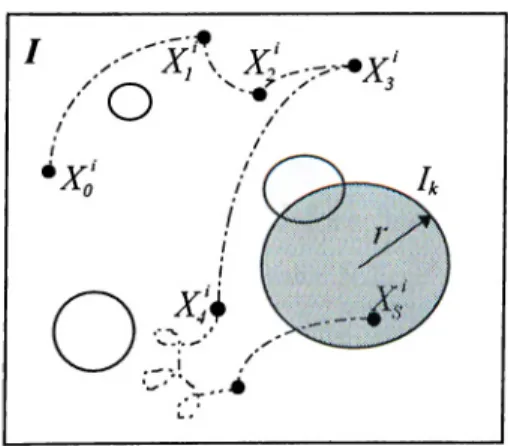
Littlewood [17] defines a program as a function whose domain is the input space of the program. He partitions the output space into two disjoint sets, as the collection of unacceptable output states, and its complement. This partition of the output space leads to a natural partition of the input space into two disjoint sets, as the collection of input states that are mapped by the program to an unacceptable output and the complement of this set. The input states selected by a user are represented with the elements of the input space selected randomly in a sequence by a random process.
.. .We shall take a program, p, to be a mapping. Here, / is the input space, i.e. the totality of all possible inputs^], and O is the output space. The failure process is illustrated in Figure 2.1pj.
Figure 2.1: A Conceptual Model of the Software Failure Process In Figure 2.1(a), we see there are certain inputs which the program p cannot exercise correctly. These comprise the subset Ip of all inputs I. In practice, a failure will be detected by a comparison between the output obtained by processing a particular input, and
^Littlewood uses input in the same meaning as input state.
C H A P T E R 2. A C O N C E P T U A L M O D E L O F S O F T W A R E FA ILU R E P R O C E S S A N D P R E L IM IN A R IE S 29
the output which ought to have been produced according to the specification of the program. Detection of failure is, of course, a non-trivial task, but we shall not concern ourselves with this prob lem here.
Here O can be taken to be the set of all outputs which can be produced by the processing o f all possible inputs represented by I. The subset of failure-prone inputs produces the subset O y of failed outputs.
We can take the conceptual model a stage further by considering the underlying faults which reside in the program p. Figure 2.1(b). If we make the reasonable assumption that each failure can be said to have been caused by one (and only one) fault, we have a partitioning of Ip into subsets corresponding to the different faults.
When we successfully remove a fault, and so change the program
p into a new program p (see Figure 2.1(c)), this has the effect of
removing certain points of / from ly . Thus, the members of the removed fault set now map into acceptable regions of O.
Operational use of a program may be thought as the selection of a trajectory of points in the space /. Typically, many inputs will be made to fix the underlying fault and if this attempt is successful we have the situation shown in the transition from Figure 2.1(b) to Figure 2.1(c).
Execution of the program then restarts (most probably in a region outside ly , since ly is typically very small), and the trajectory of successive inputs continues until the next failure when the fixing operation is repeated.
The result is a sequence of programs, p i,p2,p3, ...,P n,...; a sequence
of successively smaller sets I } . j j ,,í y ,...,l y ,...· , a sequence of out put sets 0 \ 0 ‘^ ,0 ^ ,...,0 ” ,...; and a sequence o f subsets of failed outputs 0\p, Oy , Oy , ...Oy, ...Cleavly, the reliability growth is de