Third-Degree B-spline solution for a nonlinear diffusion Fisher’s
equation
Nazan Caglar
1, Hikmet Caglar
2, and Muge Iseri
11
Faculty of Economic and Administrative Science, Istanbul Kultur University, 34156 Atakoy Istanbul, Turkey
2Department of Mathematics - Computer, Istanbul Kultur University, 34156 Atakoy Istanbul, Turkey
Abstract— Non-linear Fisher’s equations are solved by
using a spline method based on B-spline in the space direction and finite difference schema in the time direction. Numerical results reveal that spline method based on B-spline is implemented and effective.
Keywords: Non-linear Fisher’s equations;Finite difference;B-spline functions;Boundary conditions.
1. Introduction
We consider the generalized Fisher’s equation:
ut(x, t) = uxx(x, t) + αu(x, t)(1 − uβ(x, t))
a < x < b, t > 0 (1) with initial condition
u(x, 0) = Φ(x), and boundary conditions
u(a, t) = g1(t), u(b, t) = g2(t)
whereα and β are constants.
The classic and simplest case of the nonlinear reaction-diffusion equation is whenβ=1. It was suggested by Fisher as a deterministic version of a stochastic model for the spatial spread of a favored gene in a population[8].
ut(x, t) = uxx(x, t) + αu(x, t)(1 − u(x, t))
a < x < b, t > 0 (2) This equation is referred to as the Fisher equation, the discovery, investigation and analysis of traveling waves in chemical reactions was first presented by Luther[9]. In the last century, the Fisher’s equation has became the basis for a variety of models for spatial spread, for example, in logistic population growth models [10 − 11], flame propagation [12 − 13], neurophysiology [14], autocatalytic chemical reactions [15 − 17], branching Brownian motion processes [18], gene-culture waves of advance [19], the spread of early farming in Europe [20 − 21], and nuclear reactor
theory [22]. It is incorporated as an important constituent of nonscalar models describing excitable media, e.g., the Belousov-Zhabotinsky reaction[23]. In chemical media, the function u(x, t) is the concentration of the reactant and the positive constant α represents the rate of the chemical reaction. In media of other natures,u might be temperature or electric potential.
The mathematical properties of equation (1) have been studied extensively and there have been numerous discus-sions in the literature. The most remarkable summaries have been provided by Brazhnik and Tyson [24]. One of the first numerical solutions was presented in literature with a pseudo-spectral approach. Implicit and explicit finite differ-ences algorithms have been reported by different authors such as Parekh and Puri and Twizell et al. A Galerkin finite element method was used by Tang and Weber whereas Carey and Shen[25] employed a least-squares finite element method. A collocation approach based on WhittakerŠs sinc interpolation function[26] was also considered in [27]. Our solution based on B-spline method. In this paper, we propose a spline difference scheme to solve eq.(2).
The theory of spline functions is a very active field of approximation theory and boundary value problems (BVPs), when numerical aspects are considered. In a series of paper by Caglar et al. [2-7] BVPs of order two, third, fourth and fifth were solved using third, fourth and sixth-degree splines. The paper is organized as follows: B-spline function is described in Section 2 briefly. In sections 3 the methods of solution of equation (2) is presented. In section 4 some numerical result, that are illustrated using MATLAB 7.0, are given to clarify the method. Concluding remarks are given in Section 5.
2. The third-degree B-splines
In this section, third-degree B-splines are used to construct numerical solutions to the Fisher equations discussed in sections 3 and 4. A detailed description of B-spline functions generated by subdivision can be found in [1].
Consider equally-spaced knots of a partition π : a = x0 < x1< ... < xn = b on [a,b]. Let S3[π] be the
polynomials onπ. That is, S3[π] is the space of third-degree
splines on π. Consider the B-splines basis in S3[π]. The
third-degree B-splines are defined as
B0(x) = 6h13 x3 0 ≤ x < h −3x3+ 12hx2− 12h2x + 4h3 h ≤ x < 2h 3x3− 24hx2+ 60h2x − 44h3 2h ≤ x < 3h −x3+ 12hx2− 48h2x + 64h3 3h ≤ x < 4h (5) Bi−1(x) = B0(x − (i − 1)h), i = 2, 3, ...
To solve hyperbolic equation,Bi , Bi′ and Bi′′evaluated at
the nodal points are needed. Their coefficients are summa-rized in Table 1.
Table 1
VALUES OFBi, Bi′and Bi′′ xi xi+1 xi+2 xi+3 xi+4
Bi 0 1/6 4/6 1/6 0 B′ i 0 -3/6h 0/6h 3/6h 0 B′′ i 0 6/6h 2 -12/6h2 6/6h2 0
3. B-spline solutions for the nonlinear
diffusion Fisher’s equation
In this section a spline method for solving the Fisher equation is outlined, which is based on the collocation approach [5]. Let
S(x) = n−1P
j=−3
CjBj(x) (6)
be an approximate solution of Eq.(1), where Ci are
unknown real coefficients and Bj(x) are third-degree
B-spline functions. Let x0, x1, ..., xn be n + 1 grid points
in the interval [a,b], so that
xi = a + ih, i = 0, 1, ..., n ; x0=a, xn= b, h = (b − a)/n.
We consider the convection-diffusion equation (1),
difference schemes for this problem considered as following:
ui+1−ui ∆t − ∂2 u ∂x2 = u(1 − u) + f (x, t) (7) where∆t = k −ku′′
i+1+ ui+1− kui+1(1 − ui+1) = ui+ kf (x, t) (8)
and the initial condition is given in (2)
u(x, 0) = f (x) = u0, (9)
Subsituting (9) in (8) then is obtained as follows
t = 0 + k −ku′′1 + u1− ku1(1 − u1) = u0+ kf (x, k) (10) t = 0 + 2k −ku′′2 + u2− ku2(1 − u2) = u1+ kf (x, k) (11) . . . . . . t = 0 + nk −ku′′n+ un− kun(1 − un) = un−1+ kf (x, k) (12)
The approximate solution of the equation (10)-(12) are sought in the form of the B-spline functionsS(x), it follows that t = 0 + k −kS1′′+ S1− kS1(1 − S1) = u0+ kf (x, k) (13) t = 0 + 2k −kS2′′+ S2− kS2(1 − S2) = u1+ kf (x, k) (14) . . . . . . t = 0 + nk −kSn′′+ Sn− kSn(1 − Sn) = un−1+ kf (x, k) (15)
and boundary conditions (3)-(4) can be written as follows
n−1 P j=−3 CjBj(0) = 0 for x = 0, (16) n−1 P j=−3 CjBj(1) = 0 for x = 1 , (17)
The spline solution of eq.(13) with the boundary conditions is obtained by solving to the following matrix equation[see 2,4]. The value of spline functions at the knots {xi}ni=0 are determined using table1. Then we can write in
matrix-vector form as follows
This leads to the non-linear system of order n + 2 given by
n−1 P j=−3 CjBj(0) = 0 for x = 0, (18) n−1 P j=−3 CjBj(1) = 0 for x = 1 , (19) −k n−1P j=−3 CjB ′′ j(x) + n−1 P j=−3 CjBj(x) − k n−1 P j=−3 CjBj(x)(1 − n−1 P j=−3 CjBj(x)) = u0+ kf (x, k) forx = 0, h, 2h, ..., 1 (20)
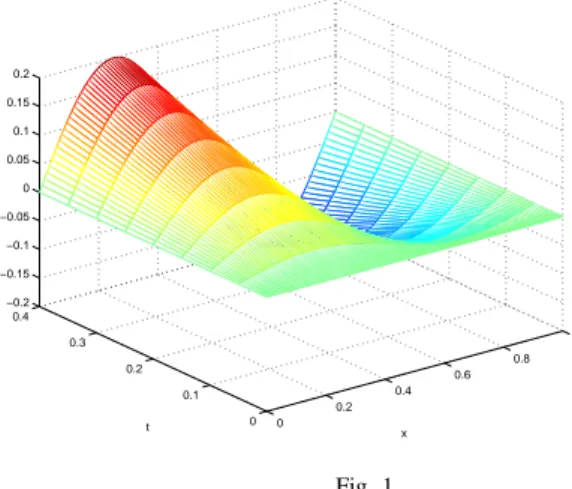
0 0.2 0.4 0.6 0.8 1 0 0.1 0.2 0.3 0.4 −0.2 −0.15 −0.1 −0.05 0 0.05 0.1 0.15 0.2 x t Fig. 1 RESULTS FORn = 121, k = 0.05
The approximate solution (8) is obtained by solving non-linear system using Levenberg-Marquardt optimization method [29] and MATLAB 6.5.
It is easy to see that, the same approximation is applied the other equations (14)-(15).
4. Numerical results
In this section, the method discussed in section 2 and 3 is tested on the following problems from the literature[7], and absolute error in the analytical solutions are calculated. All computations were carried out using MATLAB 6.5. Problem 1.
We consider a 1-D Fisher’s diffusion partial differential equation ∂u ∂t − ∂2 u ∂x2 = u(1 − u) + f (x, t) , 0 ≤ x ≤ 1 , t > 0 , (23) with the initial conditions,
u(x, 0) = 0 , 0 ≤ x ≤ 1 , (24) and the boundary conditions atx = 0 and x = 1 of the form
u(0, t) = u(1, t) = 0, t ≥ 0 . (25) The exact solution of this problem is u(t, x) = 0.5tsin2πx . The observed maximum absolute errors for various values of n and for a fixed value of k=0.05 are given in Table 1. The numerical results are illustrated in Figure 1.
Table 1. Comparison of the Numerical solution with the exact solution at different n and k=0.05
n k = 0.05 21 1.5944141x10⁻³ 41 4.0001700x10⁻⁴ 61 1.7790142x10⁻⁴ 121 4.4492962x10⁻⁵ 191 1.7748496416−5
5. Conclusions
A family of B-spline methods has been considered for the the numerical solution of the Fisher equations . The third-degree B-spline has been tested on the Fisher problem, and have tabulated the maximum absolute errors for different values of n . As is evident from the numerical results, the present method approximate the exact solution very well. Also the numerical results are illustrated in figures. The implementation of the present method is more computational than other numerical techniques.
References
[1] C. de Boor, A Practical Guide to Splines, 108,Springer-Verlag, New York, 1978.
[2] H. Caglar, M. Ozer, N.Caglar, The numerical solution of the one-dimensional heat equation by using third degree B-spline functions, Chaos Solitons Fract., 38, 1197 ˝U1201(2008).
[3] Caglar HN, Caglar SH, Twizell EH. The numerical solution of third-order boundary-value problems with fourth-degree B-spline functions. Int J Comput Math ,71,373 ˝U81(1999).
[4] Caglar HN, Caglar SH, Twizell EH. The numerical solution of fifth-order boundary-value problems with sixth-degree B-spline functions. Appl Math Lett 12,25 ˝U30(1999).
[5] Caglar N, Caglar H, Cagal B. Spline solution of nonlinear beam problems. J Concrete Appl Math 1(3),253 ˝U9(2003).
[6] Caglar H, Caglar N, Elfaituri K. B-spline interpolation compared with finite difference, finite element and finite volume methods which applied to two-point boundary value problems. Appl Math Comput, 175,72 ˝U9(2006).
[7] Caglar N, Caglar H. B-spline solution of singular boundary value problems. Appl Math Comput 182,1509 ˝U13(2006).
[8] R.A. Fisher, The wave of advance of advantageous genes, Ann. Eugen. 7 (1937) 353-369.
[9] R.L. Luther, Ra´l umliche Fortpflanzung Chemischer Reaktinen, Z. fu´l r Elektrochemie und angew, Phys. Chem. 12 (1906) 506-600.
[10] J.D. Murray, Lectures on Non-linear-Differential-Equations Models in Biology, Oxford University Press, London, 1977.
[11] N.F. Britton, Reaction-Diffusion Equations and Their Applications to Biology, Academic Press, New York, 1986.
[12] D.A. Frank-Kamenetskii, Diffusion and Heat Exchange in Chemical Kinetics, Princeton University Press, Princeton, NJ, 1955.
[13] F.A. Williams, Combustion Theory, Addison-Wesley, Reading, MA, 1965.
[14] H.C. Tuckwell, Introduction to Theoretical Neurobiology, Cambridge Studies in Mathematical Biology, vol. 8, Cambridge University Press, Cambridge, UK, 1988.
[15] H. Cohen, Nonlinear diffusion problems, in: A.H. Taut (Ed.), Studies in Applied Mathematics, MAA Studies in Mathematics, vol. 7, Mathematical Association of America, 1971, pp. 27-64 (distributed by Prentice-Hall, Englewood Cliffs, NJ).
[16] P.C. Fife, J.B. McLeod, The approach of solutions of nonlinear diffusion equations to travelling front solutions, Arch. Ration. Mech. Anal. 65 (1977) 335-361.
[17] D.G. Aronson, H.F. Weinberger, Nonlinear diffusion in population genetics, combustion, and nerve pulse propagation in: J.A.Goldstein (Ed.), Partial Differential Equations and Related Topics, Lecture Notes in Mathematics, vol. 446, Springer, Berlin, 1975,pp. 5-49.
[18] M.D. Bramson, Maximal displacement of branching Brownian motion, Comm. Pure Appl. Math. 31 (1978) 531-581.
[19] K. Aoki, Gene-culture waves of advance, J. Math. Biol. 25 (1987) 453-464.
[20] A.J. Ammerman, L.L. Cavalli-Sforza, Measuring the rate of spread of early farming, Man 6 (1971) 674-688.
[21] A.J. Ammerman, L.L. Cavalli-Sforza, The Neolithic Transition and the Genetics of Populations in Europe, Princeton University Press, Princeton, 1983.
[22] J. Canosa, Diffusion in nonlinear multiplicative media, J. Math. Phys. 10 (1969) 1862-1868.
[23] J.J. Tyson, P.C. Fife, Target patterns in a realistic model of the Belousov ˝UZhabotinskii reaction, J. Chem. Phys. 73 (1980) 2224-2257.
[24] P. Brazhnik, J. Tyson, On traveling wave solutions of FisherŠs equation in two spatial dimensions, SIAM J. Appl. Math. 60 (2) (1999) 371-391.
[25] G.F. Carey, Y. Shen, Least-squares finite element approximation of FisherŠs reaction ˝Udiffusion equation, Numer. Methods Part. Differ. Eq. 11 (1995) 175-186.
[26] J.P. Boyd, Chebyshev and Fourier Spectral Methods, Dover, New York, 2000.
[27] K. Al-Khaled, Numerical study of FisherŠs reaction ˝Udiffusion equation by the Sinc collocation method, J. Comput. Appl. Math. 137 (2001) 245-255.
[28] J. Rashidinia, R. Mohammadi, Non-polynomial cubic spline methods for the solution of parabolic equations, International Journal of Comp. Math. 85(5)(2008) 843-850.
[29] Fletcher R. Practical methods of optimization. A Wiley-Interscience Publication;1987.