Genelleştirilmiş Benjamin-Bona-Mahony denklemine Galerkin metodunun bir uygulaması

An Application of Galerkin Method to Generalized Benjamin-Bona-Mahony-Burgers Equation

Turgut AK

Yalova University, Armutlu Vocational School, Department of Food Processing, Yalova, Türkiye, akturgut@yahoo.com

Abstract

In this study, Galerkin finite element method is applied to generalized Benjamin-Bona-Mahony-Burgers (gBBM-B) equation. Quadratic B-spline functions are used as interpolation function. Stability analysis is investigated based on von Neumann theory. The performance of the proposed method is checked by two test problems with zero boundary conditions. As a result, it is observed that applied method is successful and efficient to show motions of some waves. 

Keywords: Benjamin-Bona-Mahony-Burgers equation, Finite element, Galerkin

method.

Genelleştirilmiş Benjamin-Bona-Mahony Denklemine Galerkin Metodunun Bir Uygulaması

Özet

Bu çalışmada, genelleştirilmiş Benjamin-Bona-Mahony (gBBM-B) denklemine Galerkin sonlu elemanlar yöntemi uygulanmıştır. İnterpolasyon fonksiyonu olarak kuadratik B-spline fonksiyonlar kullanılmıştır. Von Neumann teorisine bağlı olarak kararlılık analizi incelenmiştir. Sıfır sınır şartları ile iki test problemi yardımıyla önerilen yöntemin

Adıyaman University Journal of Science

dergipark.gov.tr/adyusci

ADYUSCI

performansı kontrol edilmiştir. Sonuç olarak, uygulanan yöntemin bazı dalga hareketlerini göstermek için başarılı ve etkili olduğu gözlenmiştir.

Anahtar Kelimeler:  Benjamin-Bona-Mahony-Burgers denklemi, Sonlu eleman, Galerkin metodu.

Introduction

The dynamics of shallow water waves is a seriously growing research area in the area of fluid dynamics. There are various models to describe the shallow water waves along lakeshores and beaches. These are Korteweg-de Vries (KdV) equation [1-3], Kawahara equation [4], equal width (EW) wave equation [5, 6], regularized long wave (RLW) equation [7, 8], Burgers equation [9, 10] and others [11, 12]. This paper will focus on the generalized Benjamin-Bona-Mahony-Burgers (gBBM-B) equation with following form

= 0.

p

t xxt xx x x

u u u u u u (1)

where u x t

 

, represents fluid velocity in the horizontal direction x , u is evolution term, _t x

u is dispersion term, u is dissipative term and _xx p x

u u is nonlinear term [13]. Also, ,

 , ,  are arbitrary constants, p is positive integer and  satisfying



























2 2 2 2 1 2 1 ₄ 2 2 3 2 2 1 2 4 1 = . 2 _{2 2} c p p p c p a p p a p p p c p        _{   }   _{ }   _              (2)

Many analytical and numerical methods including finite difference method [14], meshless method [15], tanh method [16], homotopy analysis method [17], exp-function method [18], tan-cot function method [19], collocation method [20] were applied to BBM-B equation in the past decades.

The organization of the paper is as follows: In Section 1, we describe quadratic B-spline interpolation function and its some properties. In Section 2, the gBBM-B equation is

considered and obtained its numerical solution using Galerkin finite element method based on quadratic B-splines. In Section 3, stability of the applied method is investigated based on von Neumann theory. In Section 4, numerical simulation is performed to check the performance of the proposed method. Finally, a brief conclusion is given in Section 5.

1. Quadratic B-splines and Properties

In this study, gBBM-B equation (1) is considered where  ,  ,  and  are arbitrary parameters, p is positive integer and the subscripts x and t denote the spatial and temporal differentiations, respectively.

Firstly, solution domain of the problem is restricted over an interval a x b  . Space interval

 

a b is separated into uniformly sized finite elements of length , h by the knots

m

x like that a=x0 <x1< ... <xN =b . Lengths of these finite elements are

1 =b a= ( _{m m}) h x x N   _{ for} = 1, 2,..., m N .

Eq. (1) is solved by taking

( , ) = 0, ( , ) = 0,

( , ) = 0, ( , ) = 0 , > 0

x x

u a t u b t

u a t u b t t (3)

homogeneous boundary conditions and

( , 0) = ( ) , .

u x f x a  x b (4)

the initial condition.

The cubic B-spline approximation functions _m( )x are defined as

2 2 2 2 1 1 2 2 2 1 1 2 2 2 1 2 ( ) 3( ) 3( ) , [ , ], ( ) 3( ) , [ , ], 1 ( ) = ( ) , [ , ], 0, . m m m m m m m m m m m m m x x x x x x x x x x x x x x x h x x x x elsewhere                  _{  }   _   (5)

functions apart from _m1( )x , _m( )x and _m1( )x are zero over the element [ ,x_m x_m1].

Each quadratic B-spline function covers three elements so that each element [ ,x_m x_m₁] is covered by three spline functions. The values of _m

 

x and its first derivative may be

tabulated as in Table 1.

Table 1. Quadratic B-splines and its derivatives at nodes x_m

x ₁ m x _ x_m x_m1 x_m2

 

m x  0 1 1 0

 

' m h x 0 -2 2 0

The set of these approximation functions



₁( ), ( ), , ( )x ₀ x N x



forms a basis for

approximate solution which will be defined over [ , ]a b . A global approximation is signified

in terms of the quadratic B-spline approximation functions as

= 1 ( , ) = N ( ) ( ), N i i i u x t  x t 



(6)

where _i( )t are time dependent parameters to be determined from the boundary and

weighted residual conditions. A typical finite interval [ ,x_m x_m1] can be converted to the interval

 

0,1 by a local coordinate transformation defined as

= _m , 0 1

h xx    (7)

In this way, it can be studied more easily on the defined new interval [0,1]. In this case, quadratic B-spline functions (5) can be defined in terms of  over the interval as the following.

 

2 1 = (1 ) , m  _  

 

2 = 1 2 2 , m      (8)

 

2 1 = . m  _  

   

1 = 1 ( , ) = m , N i i i m u  t    t  



(9)

where _m1, _m, _m1 act as element parameters and B-splines _m1, _m, _m1 as element shape functions.

Using trial function (6) and quadratic splines (5), the values of u and '

u at the knots

are determined in terms of the element parameters _m by



, =



= 1 , N m m m m u x t u  _  1 1 2 = ( _{ }).    m m m u h  

where the symbol “ ” denotes first differentiation with respect to x . The splines _m( )x and

its first derivative vanish outside the interval [x_m1,x_m2].

2. Implementation of The Method

By applying the Galerkin method to the Eq. (1) with weight function ( )w x , the weak

form of Eq. (1) is obtained as

( ) = 0. b p t xxt xx x x aw u u u u u u dx



(10)

For a single element [ ,x_m x_m₁], the following equation is obtained by using transformation (7) into the equation (10)

1 2 2 0 1 1 1 1 = 0. p t t w u u u u u u d h   h   h   h     _  _  _  _            _{       }   



(11)

Also, Eq. (11) can be written as

1 1 2 3 4 0 = 0. p t t w u_ a u_ a u_ a u_ a u u__d



(12) where a₁= ₂ h  _, 2= 2 a h  _, 3= a h  _, 4 = a h  _and = p m

z u . Integrating Eq. (12) by parts and

1 _{1 1}

1 2 3 4 1 0 2 0

0[wuta w u ta w u  a wu a z wu dm ] a wut| a wu | = 0.



(13)

Taking the weight function as quadratic B-spline shape functions given by Eq. (5) and substituting approximation (9) in integral equation (13) with some manipulation, the element contributions are obtained in the form

1 _{1 1} 1 1 1 0 0 0 , = 1 1 _{1 1 1} 1 2 ₀ 3 ₀ 4 ₀ 2 0 , = 1 | | = 0. m ' ' ' _e i j i j i j j i j m m _{' '} ' ' ' e i j i j m i j i j j i j m d a d a a d a d a z d a                           _{ }         _    _  

 











 (14)

In matrix notation, this equation becomes









1 ] 2 3 4 2 = 0, e e e e e e e e m A a B C  _a B  a a z D a C _ (15) where e = ( ₁ m    , m , 1) T m

  are the element parameters and the dot denotes

differentiation with respect to t . The element matrices e, e, e

A B C and D are given by the e

following integrals: 1 0 6 13 1 1 = = 13 54 13 30 1 13 6 e ij i j A   d          



1 0 2 1 1 2 = = 1 2 1 3 1 1 2 e ' ' ij i j B   d     _{ }        



1 0 1 1 0 = | = 2 1 2 1 0 1 1 e ' ij i j C      _        

1 0 3 2 1 1 = = 8 0 8 6 1 2 3 e ' ij i j D  d    _        



where the suffices i , j take only the values m , m , 1 m for the typical element 1

1

[ ,x_m x_m]. A lumped value for  and  are found from ( ₁) / 2p p

m m u u  as 1 1 1 = ( 2 ) . 2 p m p m m m   _    _ (16)

By assembling all contributions from all elements, Eq. (15) leads to the following matrix equation;









1 ] 2 3 4 m 2 = 0, A a B C  _a B a a Da C_ (17) where  = (_1, ₀, ..., N1, ) T N

 are global element parameters. The rows of matrices

A , B , C and



a3a4 m



D have the following form:











 





 





 

 



3 4 1 3 4 1 3 4 2 3 4 1 3 4 3 3 4 2 3 4 3 3 4 3 1 = (1, 26,66, 26,1), 30 2 = 1, 2,6, 2, 1 3 = (0,0,0,0,0), , 2 8 , 1 = 3 3 , 6 8 2 , A B C a a a a a a D a a a a a a a a a a                      _{  }            (18) where

1 1 1 2 1 2 3 1 2 3 1 = ( 2 ) , 2 1 = ( 2 ) , 2 1 = ( 2 ) . 2 p m m m p p m m m p p m m m p                          (19)

Replacing the time derivative of the parameter  by Crank-Nicolson formulation and parameter  by usual forward finite difference approximation



1





1



1 1 = , = 2 n n n n t    _    _   ₍₂₀₎

into Eq. (17), it gives the (N  2) (N2) matrix system

















1 1 2 3 4 2 1 2 3 4 2 2 = , 2 n m n m t A a B C a B a a D a C t A a B C a B a a D a C       _{        }  _{   }     _{        }  _{   }    (21)

where t is time step. Applying the boundary conditions (3) to the system (22), a N N matrix system is obtained. This system is efficiently solved with a variant of the Thomas algorithm. A typical member of the matrix system (22) may be written in terms of the nodal parameters n _and n1 _as 1 1 1 1 1 1 2 2 1 3 4 1 5 2 = 5 2 4 1 3 2 1 1 2 n n n n n n n n n n m m m m m m m m m m                                          (22) where

















3 4 1 2 1 3 4 1 2 2 3 1 2 3 4 1 2 4 3 4 1 2 5 2 1 = , 30 3 3 12 10 4 2 26 = , 30 3 3 12 66 = 4 2 , 30 10 4 2 26 = , 30 3 3 12 2 1 = , 30 3 3 12 m m m m a a t a a t a a t a a t a a t a a t a a t a a t a a t                                     (23)

which all depend on n_{. The initial vector of parameters} 0 0 1

= (

 _ ,  , 0₎

N

 must be determined to iterate the system (22). To do this, the approximation is rewritten over the interval [ , ]a b at time = 0t as follows:

0 = 1 ( , 0) = N ( ) N m m m u x  x 



(24)

where the parameters 0 m

 will be determined. u_N( , 0)x are required to satisfy the following

relations at the mesh points x for _m m= 0,1, , N ,

( ,0) = ( ,0), N m m u x u x 0 ( , 0) = ( , 0) = 0. ' ' N N u x u x (25)

The above conditions lead to a matrix system of the form

0 1 0 0 0 0 0 1 1 0 1 1 _{( ,0)} 1 1 _{( ,0)} = ( ,0) 1 1 _{( ,0)} ' N N N N N N N N u x u x u x u x                                                      _{ }    _

3. Stability of the Scheme

The stability analysis is based on the von Neumann theory. The growth factor  of the error in a typical mode of amplitude

= ,

n n imkh

m e

  (26)

where h the element size and k is the mode number, is determined from a linearization of the numerical scheme. Substituting the Fourier mode (26) into (27) gives the following equality                     2 1 1 2 1 1 1 1 1 1 2 3 4 5 2 1 1 2 5 4 3 2 1 = . i m kh i m kh i m kh i m kh i m kh n n n n n i m kh i m kh i m kh i m kh i m kh n n n n n e e e e e e e e e e                                          (27) where

































1 1 2 2 3 3 4 4 5 5 = 1 , = 1 , = 26 2 2 10 , = 26 2 2 10 , = 66 6 6 , = 66 6 6 , = 26 2 2 10 , = 26 2 2 10 , = 1 , = 1 , m m m m m m m m E M K z E M K z E M K z E M K z E M E M E M K z E M K z E M K z E M K z                                                               (28) and 2 2 20 10 5 = , = , = . 2 t E M K h h h    (29) Now, if Euler’s formula

 

 

= cos sin ,

ikh

e kh i kh (30)

is used in Eq. (27) and this equation is simplified to the following growth factor:

1 2 = i , i        (31) in which



 









 















1 2 = 66 6 6 52 4 4 cos( ) 2 2 2 cos(2 ), = 66 6 6 52 4 4 cos( ) 2 2 2 cos(2 ), = 20 _m sin( ) 2 _m sin(2 ). E M E M kh E M kh E M E M kh E M kh K z kh K z kh                           (32)

The von Neumann criterion for stability | | 1  will be satisfied when



 









₆₆ 2 _{60 52} 2 _{40 cos( )} 2 _{20 cos(2 ) > 0.}



h t h t kh h t kh

         (33)

4. Results and Discussion

Numerical results of the gBBM-B equation are obtained for two problems with zero boundary conditions.

Example 1. Consider gBBM-B equation (1) with boundary condition

u( 1, ) = (1, ) = 0 , t u t t

 

0,3 (34) and initial condition

u x( , 0) =sech k x_



x₀



_ , x 



1,1 .



(35) The parameters are taken as  = 1 , = 1 ,  = 1, a₁= 1, c= 1, h= 0.01 and

= 0.01

t

 . Also, coefficient of dissipative term is chosen as  = 0.61 , 1.16, 1.49, 1.75

 for p= 1,3,5, 7, respectively. Amplitudes of the initial solitary waves are amp= 1.

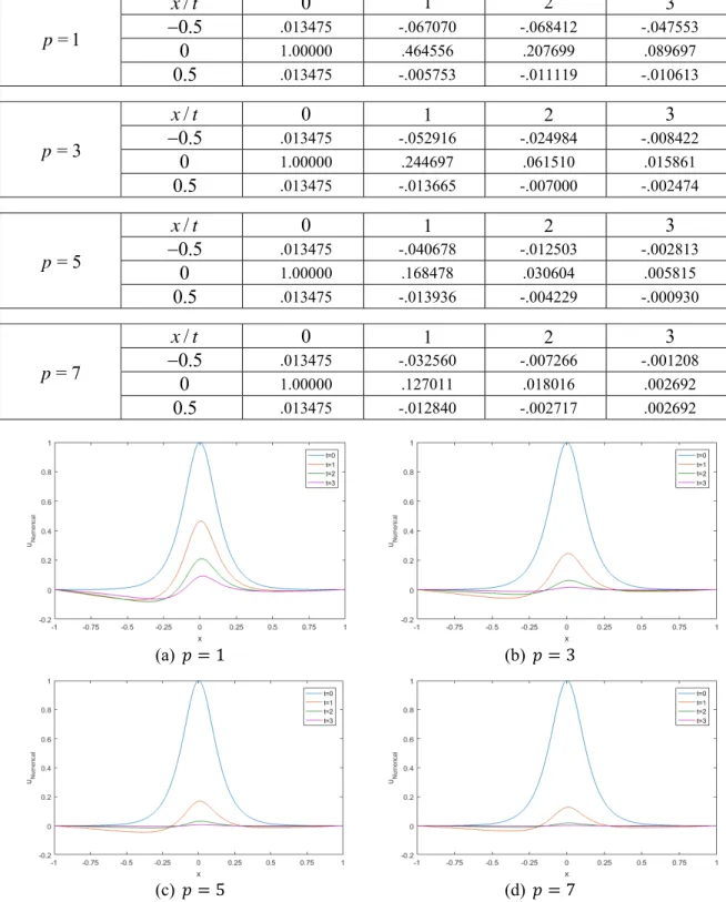
Numerical solution of Eq. (1) is given in Table 2 for some values of x in selected times. It can be observed from Figure 1, the height of the solution waves to u is more and more low with time elapsing according to the effect of dissipative term u and its coefficient. _xx

Also, the wave is faster damping as the nonlinear effect increases. Because, coefficient of dissipative term  is based on degree of the nonlinearity from Eq. (2) .

Table 2. Numerical results of Example 1 with different values of p = 1 p / x t 0 1 2 3 0.5  .013475 -.067070 -.068412 -.047553 0 1.00000 .464556 .207699 .089697 0.5 .013475 -.005753 -.011119 -.010613 = 3 p / x t 0 1 2 3 0.5  .013475 -.052916 -.024984 -.008422 0 1.00000 .244697 .061510 .015861 0.5 .013475 -.013665 -.007000 -.002474 = 5 p / x t 0 1 2 3 0.5  .013475 -.040678 -.012503 -.002813 0 1.00000 .168478 .030604 .005815 0.5 .013475 -.013936 -.004229 -.000930 = 7 p / x t 0 1 2 3 0.5  .013475 -.032560 -.007266 -.001208 0 1.00000 .127011 .018016 .002692 0.5 .013475 -.012840 -.002717 .002692 (a) 𝑝 1 (b) 𝑝 3 (c) 𝑝 5 (d) 𝑝 7

Example 2. Consider gBBM-B equation (1) with boundary condition

u( 4, ) = (4, ) = 0 , t u t t



0,0.5



(36) and initial condition

u x( ,0) = sin

 

x , x 



4, 4 .



(37) The parameters are chosen as  = 1 , = 1 ,  = 1, a₁= 1, c= 1, h= 0.01 and

= 0.01

t

 . Also, coefficient of dissipative term is taken as  = 0.61 , 1.34, 1.75, 2.07

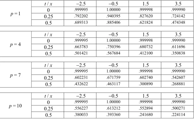
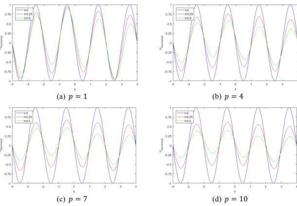
 for p= 1, 4, 7,10, respectively. Numerical solution of Eq. (1) is given in Table 3 for some values of x in selected times. Figure 2 shows that the height of the numerical approximation to u decreases as time progresses. It can be seen from Eq. (2), the effect of the dissipative term u is based on value of p . So, the height of the solution waves to u _xx

decreases faster as nonlinearity of Eq. (1) increases.

Table 3. Numerical results of Example 2 with different values of p

= 1 p / t x 2.5 0.5 1.5 3.5 0 .999995 1.00000 .999998 .999990 0.25 .792202 .940395 .827620 .724142 0.5 .689313 .885406 .621824 .474348 = 4 p / t x 2.5 0.5 1.5 3.5 0 .999995 1.00000 .999998 .999990 0.25 .663783 .750396 .680732 .611696 0.5 .501421 .567684 .412100 .350838 = 7 p / t x 2.5 0.5 1.5 3.5 0 .999995 1.00000 .999998 .999990 0.25 .602231 .671759 .602740 .542607 0.5 .432622 .463117 .300890 .268881 = 10 p / t x 2.5 0.5 1.5 3.5 0 .999995 1.00000 .999998 .999990 0.25 .556227 .613212 .552894 .500271 0.5 .380033 .393360 .241680 .224114

(a) 𝑝 1 (b) 𝑝 4

(c) 𝑝 7 (d) 𝑝 10

Figure 2. Numerical solution of u x t( , ) with different values of p for Example 2

5. Conclusion

 

In this paper, Galerkin finite element method based on quadratic B-spline interpolation function is applied to gBBM-B equation. Stability analysis is investigated based on von Neumann theory. Then, it is showed that the applied method is conditionally stable. Also, two test problems with zero boundary conditions is successfully studied to prove performance of the method. Consequently, it can be said that this method is a reliable method for calculating the numerical solutions of similar type non-linear equations and representing similar type waves.

References

[1] Korteweg, D.J., de Vries, G., On the change of form of long waves advancing in a

rectangular canal, and on a new type of long stationary wave, Philosophical Magazine, 39,

422-443, 1895.

[2] Triki, H., Ak, T., Moshokoa, S.P., Biswas, A., Soliton solutions to KdV equation

with spatio-temporal dispersion, Ocean Engineering, 114, 192-203, 2016.

[3] Triki, H., Ak, T., Biswas, A., New types of soliton-like solutions for a second order

wave equation of Korteweg-de Vries type, Applied and Computational Mathematics, 16(2),

168-176, 2017.

[4] Karakoc, S.B.G., Zeybek, H., Ak, T., Numerical solutions of the Kawahara

equation by the septic B-spline collocation method, Statistics, Optimizatin and Information

Computing, 2, 211-221, 2014.

[5] Raslan, K.R., Collocation method using quartic B-spline for the equal width (EW)

equation, Applied Mathematics and Computation, 168(2), 795-805, 2005.

[6] Saka, B., Dag, I., Dereli, Y, Korkmaz, A., Three different methods for numerical

solution of the EW equation, Engineering Analysis with Boundary Elements, 32(7), 556-566,

2008.

[7] Inan, B., Bahadir, A.R., A fully implicit finite difference scheme for the regularized

long wave equation, General Mathematics Notes, 33(2), 40-59, 2016.

[8] Lu, C., Huang, W., Qiu, J., An adaptive moving mesh finite element solution of the

regularized long wave equation, Journal of Scientific Computing, 74(1), 122-144, 2018.

[9] Inan, B., Bahadir, A.R., Numerical solution of the one-dimensional Burgers’

[10] Mittal, R.C., Tripathi, A., Numerical solutions of two-dimensional Burgers’

equations using modified Bi-cubic B-spline finite elements, Engineering Computations,

32(5), 1275-1306, 2014.

[11] Ak, T., Karakoc, S.B.G., A numerical technique based on collocation method for

solving modified Kawahara equation, Journal of Ocean Engineering and Science, 3(1),

67-75, 2018.

[12] Ak, T., Aydemir, T., Saha, A., Kara, A.H., Propagation of nonlinear shock waves

for the generalized Oskolkov equation and its dynamic motions in presence of an external periodic perturbation, Pramana-Journal of Physics, 90:78, 1-16, 2018.

[13] Sierra, C.A.G., Closed form solutions for a generalized Benjamin-Bona-Mahony-Burgers equation with higher-order nonlinearity, Applied

Mathematics and Computation, 234, 618-622, 2014.

[14] Omrani, K., Ayadi, M., Finite difference discretization of the

Benjamin-Bona-Mahony-Burgers equation, Numerical Methods for Partial Differential

Equations, 24(1), 239-248, 2008.

[15] Dehghan, M., Abbaszadeh, M., Mohebbi, A., The numerical solution of nonlinear

high dimensional generalized Benjamin-Bona-Mahony-Burgers equation via the meshless method of radial basis functions, Journal Computers Mathematics with Applications, 68(3),

212-237, 2014.

[16] Alquran, M., Al-Khaled, K., Sinc and solitary wave solutions to the generalized

Benjamin-Bona-Mahony-Burgers equations, Physica Scripta, 83, 065010, 2011.

[17] Fardi, M., Sayevand, K., Homotopy analysis method: A fresh view on

Benjamin-Bona-Mahony-Burgers equation, The Journal of Mathematics and Computer

[18] Ganji, Z.Z., Ganji, D.D., Bararnia, H., Approximate general and explicit solutions

of nonlinear BBMB equations by Exp-function method, Applied Mathematical Modelling,

33, 1836-1841, 2009.

[19] Jawad, A.J.M., New exact solutions of nonlinear partial differential equations

using tan-cot function method, Studies in Mathematical Sciences, 5(2), 13-25, 2012.

[20] Arora, G., Mittal, R.C., Singh, B.K., Numerical soltion of BBM-Burger equation

with quartic B-spline collocation method, Journal of Engineering Science and Technology,

Special Issue on (ICMTEA 2013), 104-116, 2014.