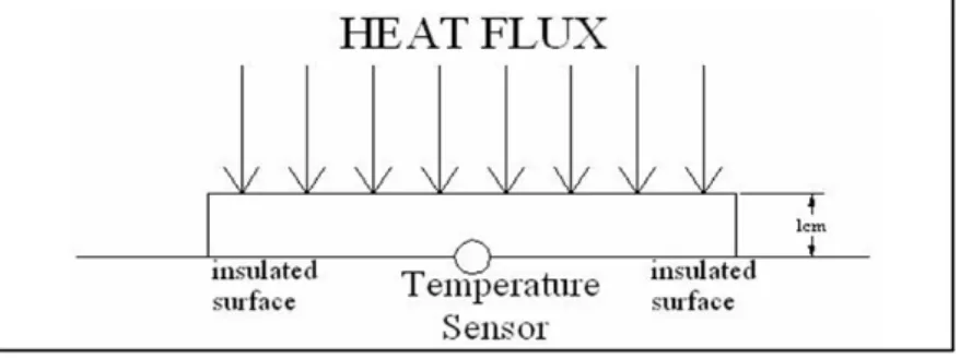
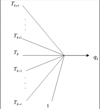
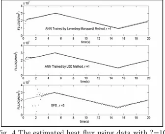
Training based method for heat flux function estimation using sensed temperatures

一、計畫主持人及共同主持人（個別型計畫）或總計畫主持人、各子計 畫主持人（整合型計畫）及協同主持人應需符合下列二項規定： （一）

We have considered the problem of linear precoder design with the aim of minimizing the sum MMSE in MIMO interfer- ence channels with energy harvesting constraints.. In the case

frequency generation, simultaneous phase matching, Q-switched Nd:YAG laser, red beam generation, modelling continuous-wave intracavity optical parametric

This study shows that noise benefits in joint detection and estimation systems can be realized to improve the perfor- mances of given suboptimal and relatively simple joint

Teacher-Related Studies \ This category consists of those studies focused on teachers in adult ESL j programs—either as the subject of the studies themselves or in the case of action

In this study, cobalt-substituted STO thin films made from a target with 30 at.% Cobalt, or STCo30 hereafter, were grown on STO substrates under different oxygen pressures, and

Ayrıca çalışmanın uygulama kısmının üçüncü bölümünde adli muhasebenin alt dalları olan “dava destek danışmanlığı”, “hile denetçiliği” ve

2577 sayılı yasa ise bu kurala koşut olarak "Kararların Sonuçları" başlıklı 28/1 maddesinde "Danıştay, bölge idare mahkemeleri, idare ve vergi mahkemelerinin esasa