Selçuk J. Appl. Math. Selçuk Journal of Vol. 7. No. 1. pp. 69-93, 2006 Applied Mathematics
A Performance Analysis For Mınımum Spanning Tree Based Genetic Algorithm Approach To Design And Optimize Distribution Network Problem
Turan Paksoy1 and Hasan Kursat Gule¸s2
1Department of Industrial Engineering, Faculty of Engineering and Architecture, Selçuk
University, Alaaddin Keykubad Campus, Konya, Turkey; e-mail: tpaksoy@ selcuk.edu.tr;
2Department of Production and Operations Management, Selcuk University, Konya,
Turkey.
Received: December 12, 2005
Summary. Supply chain management encompasses a complex business rela-tions network that contains synchronized inter and intra organizational efforts to optimizing forward flow of materials and reverse flow of knowledge through the overall production and distribution system from raw material suppliers to the last customers. Thus, one of the vital issues in supply chain management is design and optimization of a large network consisting of various business enti-ties such as suppliers, manufacturers, distribution centers and customers. In the literature, this design problem is generally defined as non polynomial-hard (NP-hard ) and genetic algorithm approach is one of the popular solution methods for the problem.
From this point of view, in this study, performance analysis for minimum span-ning based genetic algorithm approach to a design and optimization of distri-bution networks problem (which is a combination of multiple-choice Knapsack problem with the capacitated location-allocation problem) in supply chain man-agement is made and optimum combination of genetic operators is searched. 162 experimentations are made by a genetic algorithm based program written in Borland Delphi 6.0. The program is run 972 times and as a result of experi-mentations, optimum combination is determined as elitist tournament /partially matching (PMX) for the problem. Furthermore, there is no statistical differ-ence at 0.05 significance level between two mutation operators, which are analyzed. Also, 50x1500 is found as optimum for the combination of population size-generation number.
Key words: Supply Chain Management; Design and Optimization of Distribu-tion Networks; Genetic Algorithms; Minimum Spanning Tree Based Approach; Performance Analysis.
1. Introduction
A supply chain is referred to as an integrated system which synchronizes a series of inter-related business processes in order to: ) acquire raw materials and parts; ii) transform these raw materials and parts into finished products; iii) add value to these products; iv) distribute and promote these products to either retailers or customers; ) facilitate information exchange among various business entities which means traditionally suppliers, manufacturers, distributors and customers as shown by Fig. 1 (Min and Zhou, 2002).
Figure1. Traditional Supply Chain Network.
Genetic Algorithms (GAs) are search and optimization algorithms based on the principles of natural evolution (Holland, 1992). GAs start with an initial set of solutions, called population. Each solution in the population is called a chromo-some (or individual), which represents a point or one potential solution in the search space (Torabi et al., 2005). A chromosome (string) is composed of genes, which represents a number of values called alleles (Chan et al., 2005a). The chromosomes are evolved through successive iterations, called generations, by genetic operators (selection,crossover and mutation) that mimic the principles of natural evolution, until some condition (generally number of populations) is satisfied. Generation by generation, the new individuals, called offspring, are created and survive with chromosomes in the current population, called par-ents, to form a new population (Torabi et al., 2005). A new chromosome may or may not be stronger than the parents. Solutions, which are selected to form offsprings, are selected according to their fitness-the more suitable they are the more chances they have to reproduce (Smirnov et al., 2004). In a GA, a fitness value is assigned to each individual according to a problem-specific objective function (Torabi et al., 2005).
Due to its ease of applicability, numerous applications of GAs has been used successfully to find optimal or sub-optimal solutions in the area of business, scientific, and engineering optimization problems for a wide variety (Jeong et al., 2002; Chan et al., 2005b). It has also emerged as one of the most efficient stochastic solution search methods for solving supply chain optimization and management problems (Table 1).
Table 1 Genetic Algorithm based studies in supply chain optimization and management.
Syarif et al. (2002) considered the traditional supply chain network in Fig 1. and developed a 0-1 mixed integer linear programming mathematical model. The design tasks of the proposed problem involve the choice of the facilities (plants and distribution centers) to be opened and the distribution network design to satisfy the demand with minimum cost. They proposed a spanning tree-based genetic algorithm by using Prüfer number representation as solution method and demonstrated the efficiency of their method by comparing experimental results of the proposed approach with those of traditional matrix-based genetic algorithm and professional software package LINDO. But they haven’t presented a performance analysis for genetic operators for proposed approach. In order to fill up this gap in literature, in this study, as an extension to Syarif et al. (2002)’s study, a performance analysis of genetic operators for minimum spanning tree based genetic algorithms to design and optimization of supply chain network problem and optimal combination of operators are determined.
The outline of this paper is organized in five sections as follows: in Section 2 the mathematical formulation of the supply chain network design problem is given. The minimum spanning tree based genetic algorithm approach developed by Syarif et al. (2002) is summarized in Section 3. Methodology and results
of experimental performance analysis is presented in Section 4. Finally, some concluding remarks are presented in Section 5.
2. Mathematical Model of the Supply Chain Network
In the multi-echelon supply chain model developed by Syarif vd. (2002), objec-tive function is minimization of the total cost of ) fixed cost of opening potential facilities (plants, distribution centers etc.) and ii) variable cost of transporting the customer demand from facilities. The problem modeled as mixed integer linear programming model below is known as NP-hard in literature, because this kind of problem can be viewed as the combination of multiple-choice Knapsack problem with the capacitated location-allocation problem simultaneously.
minX X + X X + X X + X + X Constraints: P
6 ∀ (Capacity constraints of suppliers) P
6 ∀ (Capacity constraints of plants) P
6 (Constraints of potential plants) P
6 ∀ (Capacity constraints of distribution centers) P
6 (Constraints of potential distribution centers) P
> ∀ (Demand constraints)
= {0 1} ∀ (0-1 variable constraints) > 0 ∀
The construction of the mathematical model requires the definition of the fol-lowing elements: indices, parameters and variables given below.
Indices:
Number of suppliers (=1,2,...) Number of plants (=1,2,...)
Number of distribution centers ( =1,2,...) Number of customers ( =1,2,...)
Parameters:
Capacity of supplier ,
Capacity of plant ,
Demand of customer ,
Unit cost of production in plant using material from supplier ,
Unit cost of transportation from plant to distribution center , Unit cost of transportation from distribution center to customer , Fixed cost for operating plant ,
Fixed cost for operating distribution center ,
An upper limit on total number of distribution centers that can be opened, An upper limit on total number of plants that can be opened„
Variables:
Quantity produced at plant using raw material in supplier , Amount shipped from plant to distribution center
Amount shipped from distribution center to customer , = ½ 1 0 = ½ 1 0
3. Minimum Spanning Tree Based Genetic Algorithm Approach In this section, a minimum spanning tree based genetic algorithm approach developed by Syarif et al. (2002) regarding multi-stage supply chain (illustrated in Fig. 1) will be introduced.
Procedure:Binary Numbers
Step 1: Generate 0-1 variables for available (possible) number of plant to open ()
Step 2: Check the number of open plants for its upper limit constraint ( ) Step 3: If it exceeds the given upper limit, close one of the opened plants that has minimum capacity
Step 4: Check whether the total capacities of the opened plants satisfies the customer demand
Step 5: If the total capacity is less than total demand, then close the facility with minimum capacity and then open closed facility with maximum capacity. Continue this process until the total capacity of facilities is enough to satisfy the customer demands.
Procedure: Feasibilty check and repairing procedure for Prüfer number Repeat the following steps, until P
∈
= P ∈
Step 1: Determine indicates how many times node ( ∈ ∪ ) used from ( )
Step 3: If P ∈
P ∈
, then select one (i ∈ S) node in ( ) and replace it with the node ( ∈ D). Otherwise, select one (i∈ D) node in ( ) and replace it with node (j ∈ S) then go to Step 1.
Below, the controlling case of whether P = [4 2 6 5 6] Prüfer number is feasible or not is dealt with.
Consequently, due to P ∈
= P ∈
, Prüfer number is feasible.
Procedure: Encoding (I-J)
Step 1: Let node be the smallest labeled leaf node in a labeled sub-tree − Step 2: Let be the first digit in the encoding as the node incident to node is uniquely determined.
Step 3: Remove node and the link from to ; thus we have a sub-tree with + -1 nodes.
Step 4: Repat the above steps, until one link is left. Thus, we produce a Prüfer number or an encoding with + -2 digits between 1 and + inclusive. Procedure: Decoding (I-J)
Step 1: Let be the original Prüfer number and let ¯ be the set of all nodes not included in , which designates as eligible nodes for consideration in building a tree.
Step 2: Repeat the process (2.1)-(2.5) until no digits left in
2.1Let be the smallest label node ¯ . Let be the leftmost digit of 2.2If and are not in the same set or , add the edge from to into the tree. Otherwise, select the next digit from that not included in the same set with . Exchange with , add the edge ( ) to the tree.
2.3Remove (or ) from and from ¯ . If (or ) does not appear anywhere in the remaining part of , put it into ¯ . Designate as no longer eligible.
2.4 Assign the available amount of units to = min { } or = min { }
2.5Update the availability = − and = −
Step 3: If no digits remains in , there are exactly two nodes, and , still elligible for consideration. Add link from to into the tree and form a tree with + -1 links.
Step 4: If no available amount of units to assign, stop. Otherwise, there are remaining supply of node and demand of node , add edge ( ) to tree and assign the available amount of units = min { } to edge. If there exists a wheel, then remove the edge that assigned zero flow. A new spanning tree is formed with + -1 edges.
4. An Experimental Performance Analysis for Minimum Spanning Tree Based Genetic Algorithm Approach
Syarif et al. (2002) demonstrated that in the solution of mixed integer multi-stages supply chain model presented in section 1, the minumum spanning tree based genetic algorithm approach is more effective considering traditional ma-trix based genetic algorithm. However, there is not an analysis of operators concerning proposed minumum spanning tree based genetic algorithm. In this study, performance analysis has been carried out by means of three different types of reproduction (roulette wheel, elitist tournament and ranking selection) and crossover (one-cut-point, uniform and partially mapped cossover) operators, two differen types of mutation operators (Inversion and displacement) and opti-mal combination of evolution mechanism tried to be find concerning determined problem.
4.1 Procedures Related To Developed Minumum Spanning Tree Based Genetic Algorithm Program
In this section, the procedures related to minumum spanning tree based genetic algorithm program that used in the solution of multi-stages mixed integer supply chain network problem are presented.
i- Main Program Procedure
Initially, general procedure (main program procedure) that is used to solve the problem is given below:
Step 1: Set the beginning population,
Step 2: Check the feasibility, repair infeasible chromosomes, Step 3: Apply the evaluation procedure,
Step 4: Apply the selection procedure, Step 5: Apply the crossover procedure, Step 6: Apply the mutation procedure,
Step 7: Determine the chromosome gives the minumum value,
ii- Procedure of Binary Numbers (Open/Closed Plant/Distribution Center) Binary numbers procedure that indicates the open/closed case of plant or dis-tribution center is as follows:
Step 1: Determine number of plant/DC available to open (J), Step 2: Determine the upper limit of plant/DC number (P0), Step 3: Determine the capacity of potential plant/DC, Step 4: Determine demands of customer,
Step 5: Generate number between 0-1 amount of J, Step 6: Add the gathered (0-1) numbers (top),
Step 7: If not top6P0then close the plant/DC that has minumum capacity. Go to Step 6,
Step 8: If top6P0then add the demands (T), Step 9: Add the capacity of open plant/DC (K),
Step 10: If not K >T, then find the plant/DC that has the maximum capacity from closed plants/DCs and open it, go to Step 6,
Step 11: If K>Tthen list the open plants/DCs and stop. iii- Procedure of Feasibility Check for Prüfer (1-2-3) Numbers
The procedure of feasibility check for Prüfer numbers is given here. In this procedure, the feasibility check is designed and infeasible chromosomes which does not satisfy the feasibility criteria are repaired as follows.
Step 1: Generate supplier label 1 to I at amount of supplier (I) and build the set
Step 2: Generate plant label from I+1 to I+J at amount of plant (J) and build the D set
Step 3: Generate DC label from I+J+1 to I+J+K at amount of DC (K) and build the T set
Step 4: Determine customer label from I+J+K+1 to I+J+K+L at amount of customer (M) and build the M set
Step 5: Determine the digit number of Prüfer 1 (I+J-2) Step 6: Determine the digit number of Prüfer 2 (J+K-2) Step 7: Determine the digit number of Prüfer 3 (L+K-2) Step 8: Create the random Prüfer 1 using labels in S and D sets Step 9: Create the random Prüfer 2 using labels in T and D sets Step 10: Create the random Prüfer 3 using labels in T and M sets
Step 11: Determine (R) value indicates how many times labels in S and D sets used in Prüfer1
Step 12: Determine (R) value indicates how many times labels in T and D sets used in Prüfer2
Step 13: Determine (R) value indicates how many times labels in T and M sets used in Prüfer3
Step 14: Determine the value of L=(R+1)
Step 15: Determine the total of L in (S/D/T) set (L). Step 16: Determine the total of L in (D/T/M) set (L).
Step 17: If (L)=(L), Prüfer 1 / Prüfer 2 / Prüfer 3 is feasible.
Step 18: If (L) not equal to (L); if (L)(L), select a random node from the first label part of the Prüfer and exchange with random node from the second part of the Prüfer. Go to Step (11/12/13).
Step 19: If (L)(L), select a random node from the second label part of the Prüfer and exchange with random node from the first label part of the Prüfer. Go to Step (11/12/13).
iv- Evaluation Procedure
The evaluation procedure could be ranked as follows:
Step 1: Initialize the beginning parameters. Take the size and elements of population from main procedure.
Step 2: Run the decoding procedure for all chromosomes in the population. Step 3: Compare the cost of population elements and determine the smallest one.
v- Decoding Procedure
The decoding procedure that helps to find out the equivalent of a solution in the code space at real solution space is defined as follows:
Step 1: Enter the beginning values. Establish S, D, T, M sets. Assign labels. Enter the capacities for Prüfer (1-2-3) (a,b)
Step 2: Read the Prüfer number
Step 3: Build the set. = (Prüfer number)
Step 4: Establish the set. = (Labels of node not take part in Prüfer) Step 5: Determine the smallest element of set ()
Step 6: Determine the element that places in the most left side of set () Step 7: If and have the same group label, move right only one square and accept as . Go to Step 6.
Step 8: Constitute an arc from to : X
Step 9: Allocate resource at amount of X =min{a,b} Step 10: Update capacities a= a- X , b= b- X Step 11: Delete from and from
Step 12: If there is not another in , add to else go to next step. Step 13: If there is an element in , then go to Step 6 else go to next step Step 14: Build an arc between two elements remain in . (r,s): Apply X and Step 12 and 13, in turn.
Step 15: If not remain any transportation greater than 0 in ago to Step 20 else go to next step
Step 16: If not remain any transportation greater than 0 in bgo to Step 20 else go to next step
Step 17: Build an arc from to : X
Step 18: Allocate resource at amount of X=min{a,b} Step 19: Update capacities a= a- X, b= b- X Step 20: Stop.
vi- Procedure of Roulette Wheel Selection
Roulette Wheel method is used along with power scaling method proposed by Gillies (1985) for the purpose of preventing the early convergence of algorithm. Step 1: Enter the beginning values.
Step 2: Apply the evaluation procedure
Step 3: Find out the greater taken value (MAXF) and increase one (MAXF+1) Step 4: = P =1 ( ( ) = − ( )) Step 5: = 0995 + ( − 1)(100 ) Step 6: 0 Step 7: 0=P0( ) Step 8: Apply ( ) = 0( ) 0
Step 9: Q(EVA) Calculate the cumulative values
Step 10: Generate [0,1] variable to population size (POPSIZE). R set, (n: counter is used as - to POPSIZE)
Step 11: Get the nelement of random number set (R), find out the element that Q(EVA) is greater than R(I) and transfer it to the next gene.
Step 12: Reiterate Step 7 up to n=POPSIZE., vii- Procedure of Selection of Elitist Tournament
The developed procedure for elitist tournament which is second selection oper-ator used in experiments is defined as follows:
Step 1: Enter the beginning value Step 2: Apply the evaluation procedure
Step 3: Find out the chromosome which fitness value is best (BEST) Step 4: Select randomly two chromosomes through population
Step 5: Compute the fitness value of selected chromosomes. Register the chromosome that fitness value is lower to the next generation
Step 6: Reiterate Step 3, 4 and 5 to population size
Step 7: If there is not BEST chromosome through the new generation, then select randomly a chromosome and add its BEST chromosome.
viii- Procedure of Ranking Selection
The developed procedure regarding ranking selection is as follows: Step 1: Enter the beginning values (popsize, maxgen, etc...) Step 2: Roulette wheel procedure
Step 3: Take the outputs of Roulette Wheel Procedure and add them outputs of Crossover Procedure.
Step 4: Add the outputs of crossover to outputs of roulette wheel Step 5: Rank the elements ascently and get the first popsize element Step 6: Mutation the elements equal to popsize
Step 7: Add the outputs of mutation to population and rank them ascently. Step 8: Get the first element equals to popsize
Step 9: If wheel number is equal or less than maximum generation number, go to Step 2
ix- Procedure of One-Cut-Point Crossover
The developed procedure of one-cut-point crossover that one of the crossover mechanisms enables to change information between chromosomes is as follows: Step 1: Enter the beginning values and crossover rate (P)
Step 2: Generate random numbers in [0,1] (r)
Step 3: If rP then send the chromosome to crossover set (CSET) Step 4: If rP go to Step 2. Do population size (POPSIZE) times. Step 5: Determine the element number of CSET set (CSN)
Step 6: If CSN is odd number, then delete the chromosome in a random CSET Step 7: Divide equally the CSET set into CSET1 and CSET2 sets.
Step 8: Determine the amount of label about Prüfer number (PRU: m+n-2) Step 9: Take the Ielement of CSET1 and CSET2 and detemine a random k integer 16 k6PRU-1
Step 10: Change the parts of Ielement of CSET1 and CSET2 which are in the right side of k digit
Step 11: Transfer recently created chromosomes to new population Step 12: Repeat Step 9, 10 and 11 up to amount of CSET1’s element x- Procedure of Uniform Crossover
The developed procedure regarding another crossing method (uniform crossover) is presented as folows:
Step 1: Enter the beginning values and crossover rate (P) Step 2: Generate random numbers in [0,1] (r)
Step 3: If rP then send the chromosome to crossover set (CSET) Step 4: If rP go to Step 2. Do population size (POPSIZE) times. Step 5: Determine the element number of CSET set (CSN)
Step 6: If CSN is odd number, then delete the chromosome in a random CSET Step 7: Divide equally the CSET set into CSET1 and CSET2 sets.
Step 8: Determine the amount of label about Prüfer number (PRU: m+n-2) Step 9: Generate random number between 0 and 1: r and if r=0 then regenerate random number. Counter=Counter+1
Step 10: Change the Counterunit of Ielement of CSET1 and CSET2 sets. Transfer chromosome to new population
Step 11: Stop when counter=PRU
xi- Procedure of Partially Mapped/Planned Crossover
The developed procedure of partially mappedcrossover is as follows: Step 1: Enter the beginning values and crossover rate (P)
Step 2: Generate random numbers in [0,1] (r)
Step 4: If rP go to Step 2. Do population size (POPSIZE) times. Step 5: Determine the element number of CSET set (CSN)
Step 6: If CSN is odd number, then delete the chromosome in a random CSET Step 7: Divide equally the CSET set into CSET1 and CSET2 sets.
Step 8: Determine the amount of label about Prüfer number (PRU: m+n-2) Step 9: Take the I element of CSET1 and CSET2
Step 10: Generate two random numbers interval of 16 k 6 PRU and 16 h 6 PRU
Step 11: Exchange the parts of chromosomes which are between h and k Step 12: Change the Counterunit of Ielement of CSET1 and CSET2 sets Step 13:When counter=PRU, transfer recently created chromosomes to YEN˙IB˙IR set and exchange YENB˙IR with CSET and create a new population then stop xii- Procedure of Inversion Mutation
Mutation has a secondary role in a genetic algorithm study. The mutation operator in genetic algorithm enables to get new chromosomes (namely, new solution points in searching space) in the batch with a minor probability by randomly changing one or several values in a chromosomes (Altıparmak, 1996). In this study, Inversion and displacement mutations that not violate feasibility when applied to chromosomes were used. The procedure relating to Inversion mutation is as follows:
Step 1: Enter beginning values and rate of mutation (P) Step 2: Generate a random number in [0,1] (r)
Step 3: If not rP then register chromosome to MSET set without any change
Step 4: If rPthen get the MUT chromosome in the population
Step 5: Generate two random integers (k1, k2) in 16k6PRU. If k1=k2,then regenerate
Step 6: Reverse the parts between k1 and k2 units in the chromosome Step 7: Check the feasibility of the offspring and repair the infeasible offspring. Step 8: Apply Step 2, 3, 4, 5, 6 and 7 in turn until MUT=POPS˙IZE
xiii- Procedure of Displacement Mutation
The developed procedure of second mutation method (displacement mutation) that not violates feasibility when applied to chromosomes is given below: Step 1: Enter beginning values and rate of mutation (P)
Step 2: Generate a random number in [0,1] (r)
Step 3: If not rP then register chromosome to MSET set without any change
Step 4: If rPthen get the MUT chromosome in the population
Step 5: Generate two random integers (k1, k2) in 16k6PRU. If k1=k2then regenerate
Step 6: Determine units that constitue the sub part in interval of k1-k2 (SUB) Step 7: Determine units that are outside of SUB set (CSUB)
Step 8: Add sub part to front of a randomly selected unit in CSUB
Step 9: Check the feasibility of the offspring and repair the infeasible offspring. Step 10: Apply Step 2, 3, 4, 5, 6, 7, 8 and 9 in turn, until MUT=POPS˙IZE 4.2 Test Problems Used in Experiments
For the purpose of establishing the sensitivity of genetic algorithm operators toward problem size and building a performance analysis, three different size of test problems are used. In this section, the characteristics of test problems are defined.
For the first problem type, a supply chain network consists of 3 suppliers, 4 customers, 5 plants and 5 distribution centers is dealt with. It is assumed that maximum plant and distribution center number available to open is 4 (Syarif et al., 2002).
For the second problem type, a supply chain network consists of 5 suppliers, 10 customers, 7 plants and 7 distribution centers is dealt with. It is assumed that maximum plant and distribution center number available to open is 5.
For the third problem, a supply chain network consists of 10 suppliers, 21 cus-tomers, 10 plants and 10 distribution centers is handled. It is assumed that maximum plant and distribution center number available to open is 6.
4.3 The Working Principle and Interface of Genetic Algorithm Based Supply Chain Management Program
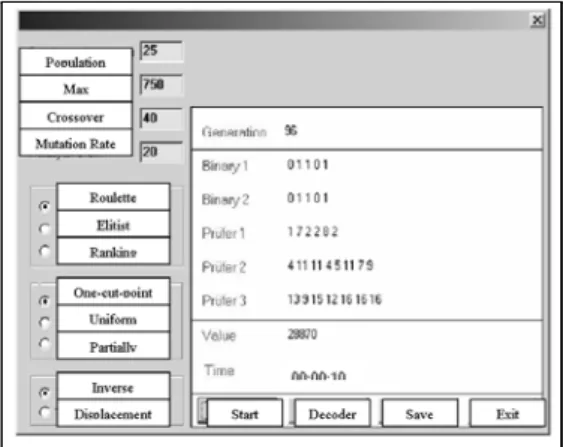
The interface of genetic algorithm based supply chain management program that is developed on Delphi 6.0 and used for experiments is illustrated in Fig. 2.
Figure 2. The Interface of Genetic Algorithm Based Supply Chain Manage-ment Program.
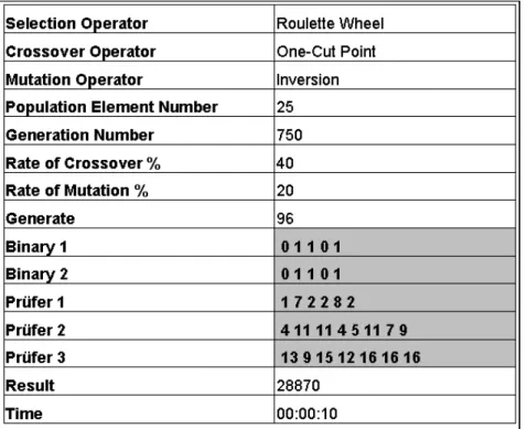
Initially user should load the new (“new problem” button) or an existing (“load problem” button) problem. User fills the capacity and fixed cost of suppliers, plants and distribution centers, customer demands, the upper limit of plants and distribution centers, unit transportation costs for each three stage to the related form regarding new problem. After problem once loaded and saved via “saved ” button, it does not necessitate to reload and able to be called back through “load problem“ button. User faces with the interface illustrated in Fig. 5.13 by means of “Solution”. In this interface, user is capable of selecting genetic algorithm operator via radio button and also able to determine number of population element and maximum generation, rate of crossover and mutation. Program runs by means of “Start ” button and obtained result is presented as chromosome (Table 2).
Table 2 Chromosome Notation of Solution Attained by Genetic Algorithm Based Program for Test 1
By “Save” button, result is saved as an Excel form. The detailed solution of Test 1 that its result is illustrated as chromosome above is pointed out in Table 3.
Table 3 The Sample Solution Results (Solved in Genetic Algorithm Based Program) of Test1.
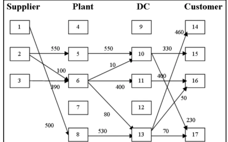
A typical figure of supply chain network designed according to obtained program result is presented below (Fig. 3).
Figure 3Supply Chain Network Build by Program for Test 1.
4.4 The Evaluation of Experiment Results
An experimental study on design and optimization of transportation networks in supply chain management is performed to determine most suitable genetic operators.162 experiments have been executed for chosen problem using three different size of test problems for combination of three population size-generation number (25x750; 30x1000; 50x1500) agreed rate of crossover % 40 and rate of mutation % 20. Program is totally run 972 times that consist of 10 run for Test 1, 5 run for Test 2, 3 run for Test 3 (Table 4).
Multi-directional variance analysis performed on SPSS 12.0 for Test 1, 2 and 3 and results were evaluated. Thus, it was purposed to determine the interaction arised between problem charecteristics (selection, crossover and mutation oper-ator, population-generation number) and folowing hypothesises were developed: Hypothesis 1: Selection operator hyphothesis
H10: There is not meaningful statistical difference between selection operators with significance level 0.05
H1: There is meaningful statistical difference between selection operators with significance level 0.05
Hypothesis 2: Crossover operator hypothesis
H20: There is not meaningful statistical difference between crossover operators with significance level 0.05
H2: There is meaningful statistical difference between crossover operators with significance level 0.05
Hypothesis 3:Mutation operator hypothesis
H30: There is not meaningful statistical difference between mutation operators with significance level 0.05
H3: There is meaningful statistical difference between mutation operators with significance level 0.05
Hypothesis 4: Population size-generation number hypothesis
H40: There is not meaningful statistical difference between combinations of population size-generation number with significance level 0.05
H4: There is meaningful statistical difference between combinations of popu-lation size-generation number with significance level 0.05
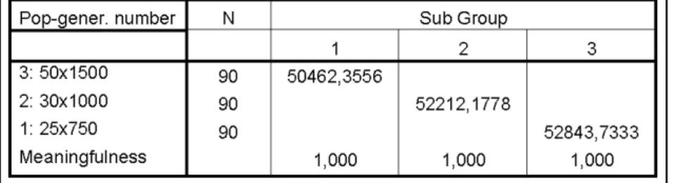
Through the multi-directional varience analysis with significance level % 5 about Test 1; selection, crossover and combination of population size-generation num-ber are statistically meaningful (Table 5.41). Therefore, H10, H20and H40hypothesis were refused with significance level 0.05 and H30was agreed. There are mean-ingful differences among groups regarding operators because of (significance level) p0.001 for selection mechanism, 0.05 for crossover and 0.001 for population-generation number. However, it is not asserted that which group or groups cause this difference merely reviewing these values. Therefore, Duncan Test that one of the test statistics enabling multiple comparisons (Altunı¸sık et al., 2002) was selected and applied on each one of three factors.(Table 5-8)
Table 5Multi-Directional Varience Analysis for Minumum Spanning Tree Based Genetic Algorithm Characteristics (Selection, Crossover and Mutation Opera-tor,
Population-Generation Number) Related to Test 1
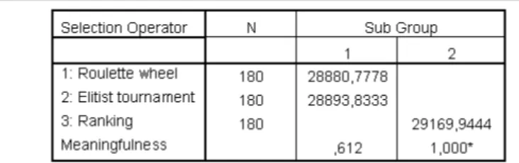
Table 6 Duncan Grouping of Selection Operator for Test 1
Two sub groups have been emerged on Duncan grouping with significance level % 5. First group consists of roulette wheel and elitist tournament methods. There is not difference between these two methods up to significance level 0.612. Therefore, it is claimed that there is not meaningful statistical difference between roulette wheel and eltist tournament methods with significance level 0.05
for Test 1. But, there is meaningful difference between ranking operator and these two operators that are in first sub group and this difference is inclened to roulette wheel and elitist tournament.
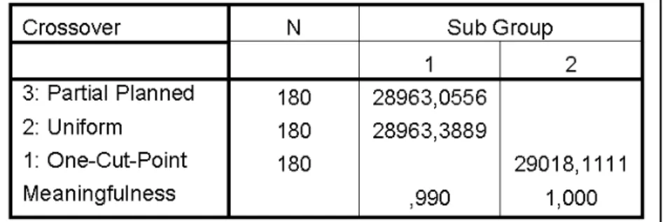
Table 7 Duncan Grouping of Crossover Operator for Test 1
Two sub groups have been emerged on Duncan grouping regarding crossover operator with significance level % 5. First group consists of partially mappedand uniform crossover methods. There is not difference between these two methods up to significance level 0.990. There is high similarity among them. Therefore, it is claimed that there is not meaningful statistical difference between partially mappedand uniform crossover methods with significance level 0.05 for Test 1. But, there is meaningful difference between one-cut-point crossover operator and these two operators that are in first sub group and this difference is inclened to partially mappedand uniform.
Table 8 Duncan Grouping of Population-Generation Number for Test 1. Two sub groups have been emerged on Duncan grouping regarding population-generation number with significance level % 5. First group consists of 50x1500 and 30x1000. There is not difference between these two combinations up to significance level 0.059. Therefore, it is claimed that there is not meaning-ful statistical difference between 50x1500 and 30x1000 combinations for Test 1. But, there is meaningful difference between 25x750 with significance level 0.05 and these two combinations that are in first sub group and this differ-ence is inclened to 50x1500 and 30x1000. It is recommended that 50x1500 and 30x1000combinations should be used for population size-generation number.
Table 9Multi-Directional Varience Analysis for Minumum Spanning Tree Based Genetic Algorithm Characteristics (Selection, Crossover and Mutation Opera-tor,
Population-Generation Number) Related to Test 2
Through the multi-directional varience analysis with significance level % 5 about Test 1; selection, crossover and combination of population size-generation num-ber are statistically meaningful (Table 9). Therefore, H10, H20and H40hypothesis were refused with significance level 0.05 and H30was agreed. There are mean-ingful differences among groups regarding operators because of (significance level) p0.001 for selection mechanism, 0.001 for crossover and 0.001 for population-generation number. Therefore, Duncan Test was applied upon each one of three factors (Table 10-12).
Three sub groups have been emerged on Duncan grouping with significance level % 5 for Test 2. These groups alternately consist of elitist tournament, roulette wheel and ranking methods. Consequently, there is meaningful statis-tical difference between roulette wheel, ranking and eltist tournament methods with significance level 0.05 for Test 2. This difference is inclened to elitist tournament.
Table 11Duncan Grouping of Crossover Operator for Test 2.
Three sub groups have been emerged on Duncan grouping regarding crossover operator with significance level % 5 for Test 2. These groups alternately consist of partially mapped crossover, uniform crossover and one-cut-point crossover methods. Consequently, there is meaningful statistical difference between par-tial planned, uniform and one-cut-point crossover methods with significance level % 5 for Test 2. This difference is inclened to partially mapped crossover.
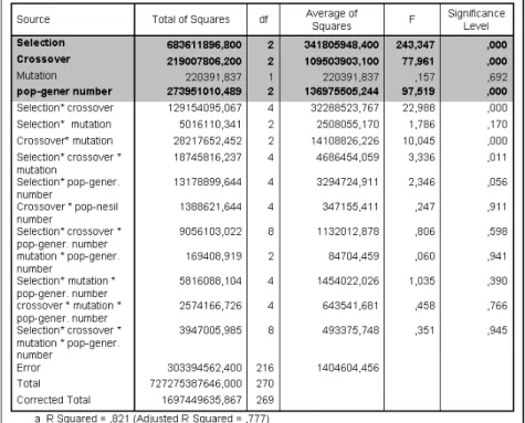
Table 12Duncan Grouping of Population-Generation Number for Test 2.
Three sub groups have been emerged on Duncan grouping regarding population-generation number with significance level % 5 for Test 2. These groups alter-nately consist of 50x1500, 30x1000 and 25x750 combinations. Consequently, there is meaningful statistical difference between 50x1500, 30x1000 and 25x750 combinations with significance level % 5 for Test 2. This difference is inclened to 50x1500. It is recommended that 50x1500 combination should be used for population size-generation number.
Table 13Multi-Directional Varience Analysis for Minumum Spanning Tree Based Genetic Algorithm Characteristics (Selection, Crossover and Mutation Operator, Population
Through the multi-directional varience analysis with significance level % 5 about Test 3; selection, crossover and combination of population size-generation num-ber are statistically meaningful (Table 13). Therefore, H10, H20and H40hypothesis were refused with significance level % 5 and H30was agreed. There are mean-ingful differences among groups regarding operators because of (significance level) p0.001 for selection mechanism, 0.001 for crossover and 0.001 for population-generation number. Therefore, Duncan Test was applied upon each one of three factors.(Table 14-16)
Table 14 Duncan Grouping of Selection Operator for Test 3.
Three sub groups have been emerged on Duncan grouping regarding selection operator with significance level % 5 for Test 3. These groups alternately consist
of elitist tournament, roulette wheel and ranking methods. Consequently, there is meaningful statistical difference between roulette wheel, ranking and eltist tournament methods with significance level % 5 for Test 3. This difference is inclened to elitist tournament.
Table 15Duncan Grouping of Crossover Operator for Test 3.
Three sub groups have been emerged on Duncan grouping regarding crossover operator with significance level % 5 for Test 3. These groups alternately con-sist of partially mappedcrossover, uniform crossover and one-cut-point crossover methods. Consequently, there is meaningful statistical difference between par-tial planned, uniform and one-cut-point crossover methods with significance level % 5 for Test 3. This difference is inclened to partially mappedcrossover.
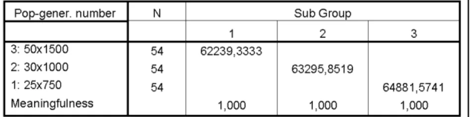
Table 16Duncan Grouping of Population-Generation Number for Test 3.
Three sub groups have been emerged on Duncan grouping regarding population-generation number with significance level % 5 for Test 3. These groups alter-nately consist of 50x1500, 30x1000 and 25x750 combinations. Consequently, there is meaningful statistical difference between 50x1500, 30x1000 and 25x750 combinations with significance level % 5 for Test 3. This difference is inclened to 50x1500. It is recommended that 50x1500 combination should be used for population size-generation number.
5. Conclusions
Genetic Algorithm is compution models that was developed to be inspired by evolution theory. In this algorithms, potential solutions of a determined problem
encode as simple chromosomes in data structure which based upon number systems that binary or not and some special processes are applied on these chromosomes in order to save critical information. Genetic algorithms that have a comprehensive application area are generally used as an optimization method (Michalewicz, 1999).
In this study, a distribution network design and optimization problem in supply chain management is dealt with by means of a minumum spanning tree based ge-netic algorithm approach. Elitist tournament selection operator/partially mapped-crossover operator is determined as most appropriate operator combination via experiments by program running. There is not meaningful statistical difference between two mutation operator reviewed with significance level % 5. Also it is established that 50x1500 combination for population-generation number com-bination must be used. The effectiveness of comcom-bination of proposed “elitist tournament selection, partially mappedcrossover operator and 50x1500 popula-tion size-generapopula-tion number” is understood when problem size increased. Acknowledgement
This paper is based on the corresponding author PhD thesis entitled “Design And Optimization Of Distribution Networks In Supply Chain Management: A Case Study And An Experimental Study Based On Genetic Algorithms”. References
1. F. Altıparmak (1996): Topological Optimization Of Communication Networks With Genetic Algorithms, Unpublished Phd Thesis, Gazi University Institute Of Natural And Applied Sciences, Ankara, Turkey.
2. R. Altuni¸sik, R. Co¸skun , S. Bayraktaro˘glu (2004): Research Methods In Social Sciences: Spss Applications, Sakarya Publishing Inc., Adapazari, Turkey (In Turkish). 3. G. Berning, M. Branderburg, K. Gürsoy, J. S. Kussi, V Mehta, F.-J. Tölle (2004): Integrated Collaborative Planning And Supply Chain Optimization For The Chemical Process Industry (I)-Methodology, Computers And Chemical Engineering, Vol. 28, Pp913-927.
4. F. T. S. Chan, S. H. Chung, S. Wadhwa (2005): A Hybrid Genetic Algorithm For Production And Distribution, Omega-The International Journal Of Management Science, Vol. 33, Pp345-355.
5. F. T. S. Chan, S. H. Chung, P .L. Y. Chan (2005): An Adaptive Genetic Algorithm With Dominated Genes For Distributed Scheduling Problems, Expert Systems With Applications, In Press.
6. A. M. Gillies (1985): Machine Learning Procedures For Generating Image Domain Feature Detectors, Doctoral Dissertation, University Of Michigan.
7. J. H. Holland (1975): Adaptation In Natural And Artificial Systems, University Of Michigan Press, 2nd Edition, Mit Press.
8. C. M. Hsu, K.-Y. Chen, M. C. Chen (2005): Batching Orders In Warehouses By Minimizing Travel Distance With Genetic Algorithms, Computers In Industry, Vol.56, Pp 169-178.
9. H.-S. Hwang (2002): Design Of Supply-Chain Logistics System Considering Service Level, Computers & Industrial Engineering, Vol. 43, Pp283-297.
10. B. Jeong, H.-S. Jung, N.-K. Park (2002): A Computerized Causal Forecasting Sys-tem Using Genetic Algorithms In Supply Chain Management, The Journal Of SysSys-tems And Software, Vol.60, Pp223-237.
11. H. J. Ko, G. W. Evans (2005): A Genetic Algorithm-Based Heuristic For The Dynamic Integrated Forward/Reverse Logistics Network For 3pls, Computers & Oper-ations Research, In Press.
12. Z. Michalewicz (1999): Genetic Algorithms + Data Structures = Evolution Pro-grams, Springer, Berlin.
13. H. Min, G. Zhou (2002): Supply Chain Modeling: Past, Present And Future, Computers & Industrial Engineering, Vol 43, Issue 1-2, Pp231-249.
14. C. Moon, J. Kim, S. Hur (2002): Integrated Process Planning And Scheduling With Minimizing Total Tardiness In Multi-Plants Supply Chain, Computers & Industrial Engineering, Vol. 43, Issue 1-2, Pp331-349.
15. A. V. Smirnov, L. B. Sheremetov, N. Chilov, J. R. Cortes (2004): Soft- Computing Technologies For Configuration Of Cooperative Supply Chain, Applied Soft Computing, Vol. 4, Pp87-107.
16. A. Syarif, Y. Yun, M. Gen (2002): Study On Multi-Stage Logistics Chain Net-work: A Spanning Tree-Based Genetic Algorithm Approach, Computers & Industrial Engineering, Vol. 43, Issue 1-2, Pp 299-314.
17. S. A. Torabi, S. M. T. Ghomi, B. Karimi (2005): A Hybrid Genetic Algorithm For The Finite Horizon Economic Lot And Delivery Scheduling In Supply Chains, European Journal Of Operational Research, In Press.
18. G. Zhou, H. Min, M. Gen (2002): The Balanced Allocation Of Customers To Multiple Distribution Centers In The Supply Chain Network: A Genetic Algorithm Approach, Computers & Industrial Engineering, Vol. 43, Pp251-261.
19. G. Zhou, H. Min, M. Gen(2003): A Genetic Algorithm Approach To The Bi-Criteria Allocation Of Customers To Warehouses, International Journal Of Production Economics, Vol. 86, Pp35-45.