Selçuk J. Appl. Math. Selçuk Journal of Vol. 13. No. 1. pp. 89-109, 2012 Applied Mathematics
Scattering by a Moving Circular Cylinder in Hertzian Electrodynamics
Burak Polat
Electrical and Electronics Engineering Department, Faculty of Engineering and Architecture,Trakya University, Edirne Turkey
e-mail: burakp [email protected]
Received Date: December 30, 2011 Accepted Date: February 8, 2012
Abstract. We provide a general formulation of electromagnetic scattering by an arbitrarily moving material object in the context Hertzian Electrodynamics, which is followed by applications to 2-D canonical problems involving perfect electric conductor and dielectric circular cylinders under plane wave incidence for various modes (uniform, harmonic, rotational) of motion.
Key words: Maxwell equations; Moving media; Hertz equations; Continuum mechanics; Frame indifference; Progressive derivatives.
2000 Mathematics Subject Classification: 78A25, 35Q60, 74A05. 1. Introduction
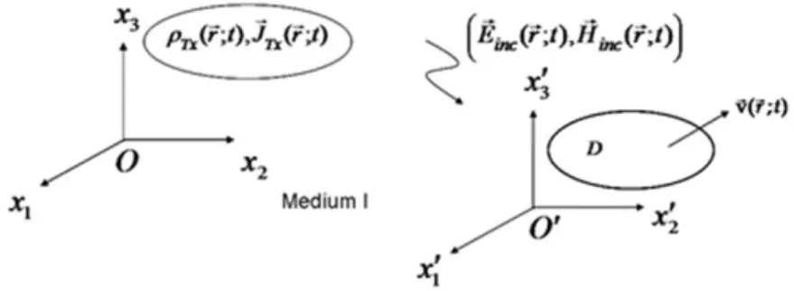
The present work is structured as a sequel of [1] where we reviewed and extended certain aspects of the mathematical foundations, axiomatic structure and prin-ciples of Hertzian Electrodynamics (HE). The introduction of a commutative property of the comoving time derivative operator in Theorem A.4 in Appendix of [1] and the corresponding Hertzian wave equations helps one construct the as-sociated boundary value problem for rigid bodies in arbitrary Euclidean motion. In that context in Section 2 we provide the general field and boundary relations for electromagnetic scattering by an arbitrarily moving material object. Specif-ically, we consider the scenario in Figure 1 where, according to an observer in Cartesian reference configuration Ox1x2x3t, the incident electromagnetic wave with fields (Einc(r; t), Hinc(r; t)) and sources (ρT x(r; t), JT x(r; t)) generated by a stationary transmitter in an ambient medium I is impinging on an object oc-cupying a region D and in arbitrary relative motion with instantaneous velocity v(r; t).
Figure 1. An illustration of a scattering problem
This is followed in the subsequent sections by applications to 2-D canonical prob-lems involving perfect electric conductor (PEC) and dielectric circular cylinders under plane wave incidence for various modes (uniform, harmonic, rotational) of motion. A theoretical comparison of similar results using the principle of special or general space-time covariance is mentioned to in Concluding Remarks. The reader is assumed to be already familiar with the terminology, definitions, postulates, theorems, etc. in [1] so that many of them shall not be repeated herein for practical reasons. In particular we shall frequently use the terms “E-frame” and “L-frame” as abbreviations of Eulerian and Lagrangian frames from fluid mechanics for denoting reference (spatial) and current (material) configurations for brevity.
2. The General Formulation of a Scattering Problem
When the coordinate transformations that describe the motion of the moving object is given, one can solve the corresponding scattering problem from an isolated moving body formally by “frame hopping”1 following the steps below:
1. Map the incoming field from E- to L-frame
2. Solve the scattered field from the associated boundary value problem in L-frame
3. Map the scattered field back from L- to E-frame
In constructing the boundary value problem in L-frame, the corresponding spa-tial/temporal jump and edge conditions are obtained from the distributional investigation of the field equations along with complementary conditions such as radiation condition, periodicity, boundedness, etc.
2.1. The Incoming Wave
In E-frame the incident fields satisfy the Maxwell equations of stationary media (2.1a,b)
curl Einc(r; t) + ∂
∂tBinc(r; t) = 0, curl Hinc(r; t) − ∂
∂tDinc(r; t) = JT x(r; t)
(2.1c,d) div Dinc(r; t) = ρT x(r; t), div Binc(r; t) = 0
Let us assume medium I simple and lossless with constitutive parameters (ε, μ). Then the incident time domain (& phasor) fields in E-frame satisfy the station-ary wave (& Helmholtz) equations
µ lap − c12 ∂2 ∂t2 ¶ µ Einc(r; t) Hinc(r; t) ¶ = µ (1/ε) grad ρT x(r; t) 0 ¶ , ¡ lap + k2¢ µ Einc(r) Hinc(r) ¶ = µ (1/ε) grad ρT x(r) 0 ¶ ,
where c = 1/√με is the phase velocity and k = ωinc/c is the wave number with angular frequency ωinc and time dependence taken as exp(−iωinct). For an observer in Cartesian L-frame Ox0
1x02x03t, the object is stationary and the sur-rounding medium I is in relative motion with an instantaneous velocity v0(r0; t). Accordingly, in L-frame the incident fields satisfy the Hertzian field and wave equations
(2.3a) curl0Einc0 (r0; t) + ♦0
♦0tBinc0 (r0; t) = 0,
(2.3b) curl0Hinc0 (r0; t) − ♦ 0
♦0tDinc0 (r0; t) = JT x0 (r0; t) (2.3c,d) div0D0inc(r0; t) = ρT x0 (r0; t), div0B0inc(r0; t) = 0
(2.4) µ lap0− 1 c2 ♦02 ♦02 ¶ µ E0 inc(r0; t) Hinc0 (r0; t) ¶ = µ (1/ε) grad0ρ0 T x(r0; t) 0 ¶ . In (2.3) the comoving time derivative of a vector A0inc(r0; t) is given by (2.5) ♦0
♦0tA0inc= ∂ ∂tA
0
inc+ v0· grad0A0inc− A0inc· grad0v0+ A0incdiv0v0. When the incident fields and sources in L-frame are monochromatic with an arbitrary time dependence, say exp (−iω0inct), then their phasors satisfy the reduced field equations (see [1], Section 7)
(2.6a,b)
curl0Einc0 (r0) − iωincBinc0 (r0) = 0, curl0Hinc0 (r0) + iωincD0inc(r0) = JT x0 (r0) (2.6c,d) div0D0inc(r0) = ρT x0 (r0), div0B0inc(r0) = 0
and the Helmholtz equations (2.7) ¡lap0+ k2¢ µ E0 inc(r0) Hinc0 (r0) ¶ = µ (1/ε) grad0ρ0 T x(r0) 0 ¶ .
2.2. The Scattered Wave
Let us express the total field in space in E- and L-frames respectively as (Etot, Htot) =
½
(Einc, Hinc) + (Esc, Hsc), in medium I (Ed, Hd), in region D
and
(E0tot, Htot0 ) = ½
(E0
inc, Hinc0 ) + (Esc0 , Hsc0 ), in medium I (Ed0, Hd0), in region D .
In L-frame of the scattered wave, i.e., with reference to the motion of region D, an L-observer senses the entire space (constituting the ambient source free medium I and region D) in motion with instantaneous velocity −v0(r0; t). Ac-cordingly, the scattered fields in medium I satisfy the Hertzian equations (2.8a,b) curl0Esc0 (r0; t) + ♦¯¯0 ♦0tB 0 sc(r0; t) = 0, curl0Hsc0 (r0; t) − ¯ ♦0 ¯ ♦0tD 0 sc(r0; t) = 0 (2.8c,d) div0D0sc(r0; t) = 0, div0Bsc0 (r0; t) = 0 (2.9) à lap0− 1 c2 ¯ ♦02 ¯ ♦0t2 ! µ E0 sc(r0; t) Hsc0 (r0; t) ¶ = 0,
where the accompanying comoving time derivative of a vector A0scis defined as (2.10) ♦¯¯0
♦0tA0sc= ∂ ∂tA
0
sc− v0· grad0A0sc+ A0sc· grad0v0− A0sc div0v0. When the scattered fields in L-frame are monochromatic with an arbitrary time dependence, say exp (−iω0
sct), then their phasors satisfy the Hertzian equations (2.11a,b) curl0Esc0 (r0) − iωincBsc0 (r0) = 0, curl0Hsc0 (r0) + iωincD0sc(r0) = 0 (2.11c,d) div0Dsc0 (r0) = 0, div0Bsc0 (r0) = 0 (2.12) ¡lap0+ k2¢ µ E0 sc(r0) H0 sc(r0) ¶ = 0.
2.3. Total Field inside the Moving Object In L-frame of the fields (E0
d, Hd0) and sources (ρ0d, Jd0) inside the moving object, the region D is sensed as stationary since the ambient medium I is observed as source-free. Therefore in region D the field equations of stationary media (2.13a,b) curl0Ed0(r0; t) + ∂ ∂tB 0 d(r0; t) = 0, curl0Hd0(r0; t) − ∂ ∂tD 0 d(r0; t) = Jd0(r0; t)
(2.13c,d) div0Dd0(r0; t) = ρd0(r0; t), div0Bd0(r0; t) = 0
are satisfied. When the region D is simple with constitutive parameters (εd, μd, σd), (2.13) yield the stationary wave equations
(2.14) µ lap0− 1 c2 d ∂2 ∂t2 − σdμd ∂ ∂t ¶ µ E0 d(r0; t) H0 d(r0; t) ¶ = µ (1/εd) grad0ρ0d(r0; t) 0 ¶ , with cd= 1/√μdεd. When the transmitted fields in L-frame are monochromatic with an arbitrary time dependence, say exp(−iω0
dt), then their phasors satisfy the reduced field equations
(2.15a,b) curl0Ed0(r0) − iωincBd0(r0) = 0, curl0Hd0(r0) + iωincDd0(r0) = Jd0(r0)
(2.15c,d) div0Dd0(r0) = ρd0(r0), div0Bd0(r0) = 0 and the Helmholtz equations
(2.16) ¡lap0+ k2d¢ µ E0 d(r0) Hd0(r0) ¶ = µ (1/εd) grad0ρ0d(r0) 0 
with kd2= ω2incεdμd+ iωincσdμd. For E-observer the field and wave equations (2.13), (2.14) read (2.17a,b) curl Ed(r; t) + ♦ ♦tBd(r; t) = 0, curl Hd(r; t) − ♦ ♦tDd(r; t) = Jd(r; t) (2.17c,d) div Dd(r; t) = ρd(r; t), div Bd(r; t) = 0 (2.18) µ lap −c12 d ♦2 ♦t2 − σdμd ♦ ♦t ¶ µ Ed(r; t) Hd(r; t) ¶ = µ (1/εd) grad ρd(r; t) 0 ¶ ,
where the accompanying comoving time derivative of a vector Ad is defined as
(2.19) ♦
♦tAd= ∂
∂tAd+ v · grad Ad− Ad· grad v + Ad div v.
When the transmitted fields in E-frame are monochromatic with an arbitrary time dependence, say exp(−iωtrt), then their phasors satisfy the reduced field equations
(2.20a,b) curl Ed(r0) − iωincBd(r) = 0, curl Hd(r) + iωincDd(r) = Jd(r)
and the Helmholtz equations (2.21) ¡lap + kd2¢ µ Ed(r) Hd(r) ¶ = µ (1/εd) grad ρd(r) 0 ¶ .
When the incident fields in L-frame are not monochromatic but possess arbi-trary waveforms which can be expressed as a superposition of monochromatic components in terms of a Fourier series or integral representation, then their each (discrete or continuous) component satisfies (2.7) individually, while similar arguments also hold in (2.12), (2.16) and (2.21).
It should be remarked that the wave numbers k, kd remain invariant in E- and L-frames, while the derivation of the Hertzian wave equations (2.4) and (2.9) are restricted to rigid bodies in arbitrary Euclidean motion as expressed by (3.18) in [1].
2.4. Boundary Relations on the Moving Object
In the context of the scattering problems investigated in the subsequent sections we shall assume the enclosure S = ∂D of the moving medium a simple interface, which might be a PEC or a dielectric interface supporting surface charges and currents ρ0
S(r0S; t), JS0(r0S; t). In these cases the distributional form of stationary field (Maxwell) equations in L- frame respectively read
(2.22a) nˆ0×hE0inc(r0S; t) + E0sc(r0S; t)i= 0 (2.22b) nˆ0×hHinc0 (r0S; t) + Hsc0 (r0S; t)i= JS0(r0S; t) (2.22c) nˆ0·hD0inc(rS0; t) + Dsc0 (r0S; t)i= ρ0S(r0S; t) (2.22d) nˆ0·hBinc0 (r0S; t) + Bsc0 (rS0; t)i= 0 and (2.23a) ˆn0×hEinc0 (rS0; t) + Esc0 (rS0; t)i= ˆn0× Ed0(r0S; t) (2.23b) nˆ0×hHinc0 (r0S; t) + Hsc0 (r0S; t)i= ˆn0× Hd0(r0S; t) (2.23c) nˆ0·hDinc0 (r0S; t) + D0sc(r0S; t)i= ˆn0· D0d(rS0; t) (2.23d) nˆ0·hBinc0 (r0S; t) + Bsc0 (rS0; t)i= ˆn0· Bd0(r0S; t).
Along with constitutive relations and radiation, edge, tip, periodicity, bounded-ness etc. type complementary conditions, the associated boundary value prob-lem can be solved uniquely to yield the L-fields (E0
sc, Hsc0 ) and ³ E0 d, Hd0 ´ , whose maps also yield the E-fields (Esc, Hsc) and (Ed, Hd).
3. TE Plane Wave Scattering by a Moving Circular PEC Cylinder In this section we consider the scattering of an incident monochromatic TE plane wave
(3.1a,b) Einc(r; t) = ˆx3eik ˆninc·re−iωinct, Hinc(r; t) = (1/Z) ˆninc× Einc(r; t) with ˆninc·r = x1cos α+x2sin α, α ∈ [0, π/2), Z =
p
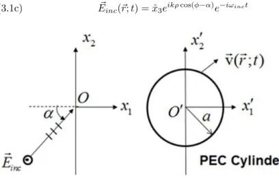
μ/ε from an infinitely long circular PEC cylinder lying along x3-axis, centered at origin and having radius a for three different modes of motion (see Figure 2). In cylindrical coordinates x1= ρ cos φ, x2= ρ sin φ the incident electrical field is represented by
(3.1c) Einc(r; t) = ˆx3eikρ cos(φ−α)e−iωinct
Figure 2. A cross section illustration of TE plane wave scattering by a moving circular PEC cylinder
3.1.Case I: Uniform Motion
Based on the coordinate transformations x1= x01+ Gt, G = const, x2,3= x02,3; ˆ
xi= ˆx0i, i = 1, 2, 3, the incoming electrical field in L-frame reads (3.2a) Einc0 (r0; t) = ˆx03eik ˆn0inc·r0e−iω0inct= ˆx0
3eikρ
0cos(φ0
−α)e−iω0inct
with ω0inc= ωinc(1−β cos α), β = G/c, where we introduced the local cylindrical coordinates ρ0 = q(x0 1) 2 + (x0 2) 2 , φ0 = tan−1(x0
known Bessel property (3.2b) eiΩ sin(ωt)= ∞ X −∞ Jm(Ω)eimωt
the incident field can be expressed as a sum of hypothetical cylindrical modes as (3.2c) E0 inc(r0; t) = ∞ P −∞ Einc0(m)(r0; t) = P∞ −∞
Einc0(m)(r0) e−iω0inct
= ˆx0 3 ∞ P −∞ Jm(kρ0) e−im(φ 0−α−π/2) e−iω0 inct.
Based on the principle of superposition for sources and fields, which stem from the linear structure of field equations, the scattered field can be considered as a superposition of modes E0 sc(r0; t) = ∞ P −∞ Esc0(m)(r0; t) = ˆx03 ∞ P −∞ Esc0(m)(r0) e−iω 0(m) sc t,
which satisfy the reduced boundary value problem (3.3)⎧ ⎪ ⎪ ⎪ ⎪ ⎪ ⎨ ⎪ ⎪ ⎪ ⎪ ⎪ ⎩ ¡ lap0+ k2¢E0(m) sc (r0) = 0, in medium I Boundary Condition : Jm(ka)e−im(φ 0−α−π/2) e−iω0 inct+ Esc0(m)¡ρ0= a, φ0¢e−iω0(m)sc t= 0, ∀φ0, t Periodicity Condition : Esc0(m)(ρ0, φ0) = Esc0(m)(ρ0, φ0+ 2π), ∀ρ0, φ0 Radiation Condition as ρ0 → ∞
From (3.3) one uniquely solves ω0inc= ω0(m)sc and (3.4) Esc0(m)(ρ0, φ0) = − Jm(ka) Hm(1)(ka) Hm(1)(kρ0) e−im(φ0−α−π/2) to get (3.5) Esc(x1, x2; t) = −ˆx3 ∞ P −∞ Jm(ka) Hm(1)(ka) Hm(1) ³ kp(x1− Gt)2+ x22 ´
× e−im(tan−1(x2/(x1−Gt))−α−π/2)e−iωinc(1−β cos α)t
In the far field of the scatterer one can substitute the asymptotic formula (3.6) Hm(1)(kρ0) ∼= r 2 πkρ0 e i(kρ0−π/4−mπ/2), kρ0>> 1 into (3.4) to get (3.7a) Esc0 (ρ0, φ0; t) ∼= ˆx03F0(φ0)e ikρ0 √ kρ0e −iω0 inct, kρ0 >> 1
with the scattering pattern (3.7b) F0¡φ0¢= −e−iπ/4 r 2 π ∞ X −∞ Jm(ka) Hm(1)(ka) e−im(φ0−α). The corresponding phasor modes of the magnetic field are derived as
Hsc0(m)(r0) = (1/iμωinc) curl0Esc0(m)(r0) = (1/iμωinc) " ˆ ρ0 ρ0(−im) − ˆφ 0 ∂ ∂ρ0 # Esc0(m)(r0). The special case ω = 0 coincides with Case I.
3.2. Case II: Harmonic Motion In this mode we consider the special case
(3.8) v(t) = G(t)ˆx1, G(t) = G cos(ωt), G = const with coordinate transformations
(3.9)
x1= x01+ F (t), F (t) = (G/ω) sin(ωt), x2= x02, x3= x03; ˆxi= ˆx0i, i = 1, 2, 3. Then the incoming electrical field in L-frame reads
(3.10) E0
inc(r0; t) = ˆx03eikˆn
0
inc·r0eiΩ sin(ωt)e−iωinct= ˆx0
3 ∞ P −∞ Jm(Ω)eikρ 0cos(φ0 −α)e−iω0(m)inc t = ˆx0 3 ∞ P −∞ ∞ P −∞ Jm(Ω)Js(kρ0) e−is(φ 0−α−π/2) e−iω0(m)inc t = ˆx0 3 ∞ P −∞ ∞ P −∞ Einc0(m,s)(r0; t) = ˆx0 3 ∞ P −∞ ∞ P −∞
Einc0(m,s)(r0) e−iω0(m)inc t
with Ω = (G/ω) k cos α, ω0(m)inc = ωinc−mω. The scattered field can be expressed in the form E0 sc(r0; t) = ˆx03 ∞ P −∞ ∞ P −∞ Esc0(m,s)(r0) e−iω 0(m)
sc t, where each (hypothetical)
mode satisfies the boundary value problem (3.11)⎧ ⎪ ⎪ ⎪ ⎪ ⎪ ⎨ ⎪ ⎪ ⎪ ⎪ ⎪ ⎩ ¡ lap0+ k2¢E0(m,s) sc (r0) = 0, in medium I Boundary Condition : Jm(Ω)Js(ka)e−is(φ 0
−α−π/2)e−iω0(m)inc t+ Esc0(m,s)¡ρ0, φ0¢e−iω0(m)sc t= 0, ∀φ0, t
Periodicity Condition : Esc0(m,s)(ρ0 = a, φ0) = Esc0(m,s)(ρ0 = a, φ0+ 2π), ∀φ0 Radiation Condition as ρ0 → ∞
from which one obtains ω0(m)sc = ω0(m)inc and (3.12) Esc0 (ρ0, φ0; t) = −ˆx03 ∞ X −∞ ∞ X −∞ Jm(Ω) Js(ka) Hs(1)(ka)
(3.13) Esc(x1, x2; t) = −ˆx3 ∞ P −∞ ∞ P −∞ Jm(Ω) Js(ka) Hs(1)(ka) Hs(1) ³ kp(x1− F (t))2+ x22 ´
× e−is(tan−1(x2/(x1−F (t)))−α−π/2)e−i(ωinc−mω)t
3.3. Case III: Rotational Motion
In this case the cylinder is assumed to rotate in counterclockwise direction with uniform angular frequency ω, which obeys the coordinate transformations
∙ x01 x0 2 ¸ = ∙ cos(ωt) sin(ωt) −sin(ωt) cos(ωt) ¸ ∙ x1 x2 ¸ , x03= x3
and linear velocity v(t) = ωaˆφ(t), ˆφ(t) = −ˆx1sin(ωt) + ˆx2cos(ωt). Inserting the polar coordinate maps ρ = ρ0, φ = ωt + φ0 in (3.1c), the incident field has the L-frame representation (3.14) E0 inc(r0; t) = ˆx03eikρ 0cos(φ0−α+ωt) e−iωinct = ˆx0 3 ∞ P −∞ Jm(kρ0) e−im(φ 0 −α−π/2+ωt)e−iωinct = ˆx0 3 ∞ P −∞ Jm(kρ0) e−im(φ 0−α−π/2) e−iω0(m)inc t = P∞ −∞ Einc0(m) (r0; t)
where we define ω0(m)inc = ωinc+ mω. For L-observer, the cylinder is stationary and the ambient medium I is rotating clockwise with linear velocity
v0(r0; t) = −ωρ0φˆ0(t), ˆφ0(t) = −ˆx01sin(−ωt) + ˆx02cos(−ωt).
That the incident field satisfies the homogeneous frame indifferent wave equation (3.15) µ lap0− 1 c2 ♦02 ♦0t2 ¶ Einc0 = 0 can be seen upon the substitutions
lap0Einc0 = xˆ03lap0³eikρ0cos(φ0−α+ωt)´e−iωinct= −k2E0
inc, v0· grad0 = −ω ∂ ∂φ0, ♦0 ♦0t = ∂ ∂t− ω ∂ ∂φ0, ♦0
♦0tEinc0 = −iωincEinc0 , 1 c2 ♦02 ♦0t2Einc0 = − ω2 inc c2 Einc0 = −k2Einc0 Then the scattered field can be expressed in the form
Esc0 (r0; t) = ∞ X −∞ Esc0(m)(r0; t) = ˆx03 ∞ X −∞ E0(m)sc (r0; t) = ˆx03 ∞ X −∞ Esc0(m)(r0) e−iω0(m)sc t,
where each mode is to be calculated from the boundary value problem (3.16) ⎧ ⎪ ⎪ ⎪ ⎪ ⎪ ⎪ ⎨ ⎪ ⎪ ⎪ ⎪ ⎪ ⎪ ⎩ µ lap0− 1 c2 ³ ∂ ∂t+ ω ∂ ∂φ0 ´2¶ E0(m)sc (r0; t) = 0, in medium I Boundary Condition : Jm(ka)e−im(φ 0
−α−π/2)e−iω0(m)inct+ Esc0(m)¡ρ0= a, φ0¢e−iω0(m)sc t= 0, ∀φ0, t
Periodicity Condition : Esc0(m)(ρ0, φ0) = Esc0(m)(ρ0, φ0+ 2π), ∀ρ0, φ0 Radiation Condition as ρ0 → ∞
We may apply the method of separation of variables proposing (3.17) Esc0(m)(r0; t) = R(m)(ρ0)Φ¡φ0¢e−iω0(m)inct.
The component describing angular variation satisfies the reduced boundary value problem
(3.18) ••Φ¡φ0¢+ v2Φ(φ0) = 0, Φ(φ0) = Φ(φ0+ 2π)
which restricts the separation constant ν to positive integer values ν = 1, 2, ... for linearly independent eigenmodes, while we choose Φv(φ0−iν(φ
0−α−π/2)
for convenience. Then the radial component satisfies the Bessel equation
(3.19) ⎛ ⎝ d2 dρ02 + 1 ρ0 d dρ0 + Ã ω0(m−ν)inc c !2 − ν 2 ρ02 ⎞ ⎠ R(m) ν = 0,
with ω0(m−ν)inc = ωinc+ (m − ν)ω, which uniquely yields ν-th order Hankel functions of the first kind Hν(1)
µ ω0(m−ν)inc
c ρ0 
under the radiation condition. Ac-cordingly, the sought for m-th mode of the scattered field can be written as (3.20) E0(m)sc (r0; t) = ˆx03 ∞ X ν=1 a(m)ν Hν(1) Ã ω0(m−ν)inc c ρ 0 !
e−iν(φ0−α−π/2)e−iω0(m)inct,
where the unknown coefficients a(m)ν are to be solved from the reduced boundary condition (3.21) ∞ X ν=1 a(m)ν Hν(1) Ã ω0(m−ν)inc c a !
e−iν(φ0−π/2) = −Jm(ka)e−im(φ
0−α−π/2)
, ∀φ0.
Based on the orthogonality property (3.22) Z 2π 0 e+ir(φ0−π/2)e−iν(φ0−π/2)dφ0= ½ 0, ν 6= r 2π, ν = r ,
of the trigonometric functions one can multiply both sides of (3.21) by e+ir(φ0−α−π/2) and integrate w.r.t. φ0 from 0 to 2π to get
2πa(m)r Hr(1) Ã ω0(m−r)inc c a ! = −Jm(ka) Z 2π 0 e+ir(φ0−π/2)e−im(φ0−π/2)dφ0 = ½ 0, m 6= r −2πJm(ka), m = r which reads (3.23) a(m)r = ½ 0, r 6= m −Jm(ka)/Hm(1)(ka), r = m and eventually (3.24) Esc0(m) (r0; t) = −ˆx03 Jm(ka) Hm(1)(ka)
Hm(1)(kρ0) e−im(φ0−α−π/2)e−iω0(m)inc t
(3.25) Esc(m)(r; t) = −ˆx3
Jm(ka) Hm(1)(ka)
Hm(1)(kρ)e−im(φ−α−π/2)e−iωinct
(3.26) Esc(r; t) = −ˆx3 "∞ X −∞ Jm(ka) Hm(1)(ka) Hm(1)(kρ)e−im(φ−α−π/2) # e−iωinct.
It is observed that the total scattered field is monochromatic, having the same angular frequency as the incident field and its expression is independent of the angular frequency of rotation ω, coinciding with the result for the stationary case ω = 0.
4. TE Plane Wave Scattering by a Moving Circular Dielectric Cylin-der
In this section we shall investigate the scattering of an incident homogeneous monochromatic TE plane wave given in (3.1) by a lossless circular dielectric cylinder with constitutive parameters (εd,μd) for the same three modes of motion as in Section 3 in a similar fashion. Therefore the same quantities already defined for the corresponding problem in Section 3 will not be repeated.
4.1. Case I: Uniform Motion
As in Section 3.1 the incident, scattered and transmitted fields in L-frame read
(4.1a) E0 inc(r0; t) = ∞ P −∞ Einc0(m)(r0; t) = P∞ −∞
Einc0(m)(r0) e−iω0inct
= ˆx03 ∞ P −∞ Jm(kρ0) e−im(φ 0−α−π/2) e−iω0inct
(4.1b)
H0inc(r0; t) = (1/Z) ˆn0inc× E0inc(r0; t) = ∞ P −∞ Hinc0(m)(r0; t) = P∞ −∞
Hinc0(m)(r0)e−iω0inct
(4.2a) Esc0 (r0; t) = ∞ X −∞ Esc0(m)(r0; t) = ∞ X −∞ Esc0(m)(r0) e−iω0(m)sc t (4.2b) Hsc0 (r0; t) = ∞ X −∞ Hsc0(m)(r0; t) = ∞ X −∞ Hsc0(m)(r0) e−iω0(m)sc t (4.3a) Ed0(r0; t) = ∞ X −∞ Ed0(m)(r0; t) = ∞ X −∞ E0(m)d (r0) e−iω0(m)d t (4.3b) Hd0(r0; t) = ∞ X −∞ Hd0(m)(r0; t) = ∞ X −∞ Hd0(m)(r0) e−iω0(m)d t
which are related by
(4.4a) Hinc0(m)(r0) = (1/iμωinc) curl0Einc0(m)(r0)
(4.4b) Hsc0(m)(r0) = (1/iμωinc) curl0Esc0(m)(r0)
(4.4c) Hd0(m)(r0) = (1/iμdωinc) curl0Ed0(m)(r0) with ω0
value problem (4.5a,k) ⎧ ⎪ ⎪ ⎪ ⎪ ⎪ ⎪ ⎪ ⎪ ⎪ ⎪ ⎪ ⎪ ⎪ ⎪ ⎪ ⎪ ⎪ ⎪ ⎪ ⎪ ⎪ ⎪ ⎪ ⎪ ⎪ ⎪ ⎪ ⎪ ⎪ ⎪ ⎪ ⎪ ⎪ ⎪ ⎪ ⎪ ⎪ ⎪ ⎪ ⎪ ⎪ ⎪ ⎪ ⎪ ⎨ ⎪ ⎪ ⎪ ⎪ ⎪ ⎪ ⎪ ⎪ ⎪ ⎪ ⎪ ⎪ ⎪ ⎪ ⎪ ⎪ ⎪ ⎪ ⎪ ⎪ ⎪ ⎪ ⎪ ⎪ ⎪ ⎪ ⎪ ⎪ ⎪ ⎪ ⎪ ⎪ ⎪ ⎪ ⎪ ⎪ ⎪ ⎪ ⎪ ⎪ ⎪ ⎪ ⎪ ⎪ ⎩ ¡ lap0+ k2¢ à E0(m)sc (r0) Hsc0(m)(r0) ! = 0, in medium I ³ lap0− 1 c2 d ∂2 ∂t2 ´Ã E0(m) d (r0; t) Hd0(m)(r0; t) ! = 0 or¡lap0+ k2 d ¢Ã Ed0(m)(r0) Hd0(m)(r0) ! = 0, in region D Boundary Conditions : Einc0(m)(ρ0= a, φ0; t) + Esc0(m)(ρ0 = a, φ0; t) ¯ ¯ ¯ tangential = Ed0(m)(ρ0= a, φ0; t)¯¯¯ tangential, ∀φ 0, t Hinc0(m)(ρ0= a, φ0; t) + H0(m) sc (ρ0= a, φ0; t) ¯ ¯ ¯ tangential = Hd0(m)(ρ0 = a, φ0; t)¯¯¯ tangential, ∀φ 0, t Periodicity Conditions : Esc0(m)(ρ0, φ0) = Esc0(m)(ρ0, φ0+ 2π), ∀ρ0, φ0 Ed0(m)(ρ0, φ0) = Ed0(m)(ρ0, φ0+ 2π), ∀ρ0, φ0 Hsc0(m)(ρ0, φ0) = Hsc0(m)(ρ0, φ0+ 2π), ∀ρ0, φ0 Hd0(m)(ρ0, φ0) = Hd0(m)(ρ0, φ0+ 2π), ∀ρ0, φ0 Boundedness Conditions : Ed0(m)(ρ0= 0, φ0) = finite, ∀φ0 Hd0(m)(ρ0= 0, φ0) = finite, ∀φ0
Radiation Condition for each mode as ρ0 → ∞ (4.5a,b) uniquely yields
(4.6) ω0(m)sc = ω0inc, ω0(m)d = ωinc and the electrical field modes can be represented by
(4.7) E 0(m) sc (ρ0, φ0) = ˆx03AmHm(1)(kρ0) e−im(φ 0 −α−π/2), Ed0(m)(ρ0, φ0) = ˆx0 3BmJm(kdρ0) e−im(φ 0 −α−π/2)
The boundary conditions (4.5c,d) require the constants Am, Bm to be solved from the system
(4.8a) Jm(ka) + AmHm(1)(ka) = BmJm(kda)
(4.8b) (k/μωinc) h Jm0 (ka) + AmHm0(1)(ka) i = (kd/μdωinc) BmJm0 (kda) to get (4.9a) Am= 1 ∆m[−J 0
(4.9b) Bm= 1 ∆m
h
−Jm0 (ka)Hm(1)(ka) + Jm(ka)Hm(1)0(ka) i
=(2i/πka) ∆m with
(4.9c) ∆m= Jm(kda)Hm(1)0(ka) − (Z/Zd) Jm0 (kda)Hm(1)(ka), while Zd =
p
μd/εd. Hence, the scattered and transmitted electrical fields in L-frame read (4.10a) Esc0 (ρ0, φ0; t) = ˆx03 ∞ X −∞ AmHm(1)(kρ0) e−im(φ 0 −α−π/2)e−iω0inct (4.10b) Ed0(ρ0, φ0; t) = ˆx03 ∞ X −∞ BmJm(kdρ0) e−im(φ 0 −α−π/2)e−iωinct (4.11a) Esc(x1, x2; t) = ˆx3 ∞ P −∞ AmHm(1) ³ kp(x1− Gt)2+ x22 ´
× e−im(tan−1(x2/(x1−Gt))−α−π/2)e−iωinc(1−β cos α)t
(4.11b) Ed(x1, x2; t) = ˆx3 ∞ P −∞ BmJm ³ kd p (x1− Gt)2+ x22 ´
× e−im(tan−1(x2/(x1−Gt))−α−π/2)e−iωinct
In the far field of the scatterer one has (3.7a) with the scattering pattern (4.12) F0¡φ0¢= e−iπ/4 r 2 π ∞ X −∞ Ame−im(φ 0 −α).
4.2. Case II: Harmonic Motion
Similar to the case in Section 3.2 the incident, scattered and transmitted fields in L-frame read (4.13a) Einc0 (r0; t) = ∞ X −∞ ∞ X −∞
Einc0(m,s)(r0) e−iω0(m)inc t
(4.13b) Hinc0 (r0; t) = (1/Z) ˆn0inc× Einc0 (r0; t) = ∞ X −∞ ∞ X −∞
Hinc0(m,s)(r0) e−iω0(m)inc t
(4.14) E0 sc(r0; t) = ∞ P −∞ ∞ P −∞ Esc0(m,s)(r0) e−iω 0(m) inc t, H0 sc(r0; t) = P∞ −∞ ∞ P −∞ Hsc0(m,s)(r0) e−iω 0(m) inc t
(4.15) E0 d(r0; t) = ∞ P −∞ ∞ P −∞ Ed0(m,s)(r0) e−iωinct, H0 d(r0; t) = P∞ −∞ ∞ P −∞ Hd0(m,s)(r0) e−iωinct with
(4.16a) Einc0(m,s)(r0) = ˆx30Jm(Ω)Js(kρ0) e−is(φ
0−α−π/2) (4.16b) E0(m,s) sc (r0) = ˆx03Am,sJm(Ω)Hs(1)(kρ0) e−is(φ 0 −α−π/2) (4.16c) Ed0(m,s)(r0) = ˆx03Jm(Ω)Bm,sJs(kdρ0) e−is(φ 0 −α−π/2) and
(4.17a) Hinc0(m,s)(r0) = (1/iμωinc) curl0Einc0(m,s)(r0) (4.17b) Hsc0(m,s)(r0) = (1/iμωinc) curl0Esc0(m,s)(r0)
(4.17c) Hd0(m,s)(r0) = (1/iμdωinc) curl0Ed0(m,s)(r0)
while Ω = (G/ω) k cos α, ω0(m)inc = ωinc− mω. The boundary conditions require the constants Am,s, Bm,sto be solved from the system
(4.18a) hJs(ka) + Am,sHs(1)(ka) i
e−iω0(m)inc t= B
m,sJs(kda)e−iωinct (4.18b) (k/μωinc) ∙ J0 s(ka) + Am,sHs(1) 0 (ka) ¸ e−iω0(m)inc t= (k
d/μdωinc) Bm,sJs0(kda)e−iωinct to get
(4.19a) Am,s= 1 ∆m,s[−J
0
s(ka)Js(kda) + (Z/Zd) Js(ka)Js0(kda)] (4.19b)
Bm,s= 1 ∆m,s
∙
−Js0(ka)Hs(1)(ka) + Js(ka)Hs(1)
0 (ka) ¸ eimωt= (2i/πka) ∆m,s eimωt with (4.19c) ∆m,s= Js(kda)Hs(1) 0
(ka) − (Z/Zd) Js0(kda)Hs(1)(ka) Hence, the scattered and transmitted electrical fields in L-frame read (4.20a) Esc0 (ρ0, φ0; t) = ˆx03 ∞ X −∞ ∞ X −∞ Am,sJm(Ω)Hs(1)(kρ0) e−is(φ 0−α−π/2) e−iω0(m)inct
(4.20b) Ed0(ρ0, φ0; t) = ˆx03(2i/πka) ∞ X −∞ ∞ X −∞ 1 ∆m,s Jm(Ω)Js(kdρ0) e−is(φ 0−α−π/2) e−iω0(m)inc t (4.21a) Esc(x1, x2; t) = ˆx3 ∞ P −∞ ∞ P −∞ Am,sJm(Ω)Hs(1) ³ kp(x1− F (t))2+ x22 ´
× e−is(tan−1(x2/(x1−F (t)))−α−π/2) e−i(ωinc−mω)t
(4.21b) Ed(x1, x2; t) = ˆx3(2i/πka) ∞ P −∞ ∞ P −∞ 1 ∆m,sJm(Ω)Js ³ kd p (x1− F (t))2+ x22 ´
× e−is(tan−1(x2/(x1−F (t)))−α−π/2) e−i(ωinc−mω)t
4.3. Case III: Rotational Motion
Similar to the case in Section 3.3 the incident fields in L-frame read
(4.22) E 0 inc(r0; t) = ∞ P −∞ Einc0(m) (r0; t) = P∞ −∞
Einc0(m)(r0) e−iω0(m)inc t,
Einc0(m) (r0) = ˆx0 3Jm(kρ0) e−im(φ 0 −α−π/2) (4.23) H 0 inc(r0; t) = ∞ P −∞ Hinc0(m)(r0; t) = P∞ −∞
Hinc0(m)(r0) e−iω0(m)inc t,
Hinc0(m)(r0) = (1/iμωinc) curl0E0(m) inc (r0)
with ω0(m)inc = ωinc+ mω. Then the scattered and transmitted fields can be considered in the form
E0 sc(r0; t) = ∞ P −∞ Esc0(m)(r0; t) = ∞ P −∞ Esc0(m)(r0) e−iω 0(m) sc t, Hsc0 (r0; t) = P∞ −∞ Hsc0(m)(r0; t) = ∞ P −∞ Hsc0(m)(r0) e−iω 0(m) sc t Ed0(r0; t) = P∞ −∞ Ed0(m)(r0; t) = P∞ −∞ Ed0(m)(r0) e−iω0(m)d t, H0 d(r0; t) = ∞ P −∞ Hd0(m)(r0; t) = P∞ −∞ Hd0(m)(r0) e−iω0(m)d t
These modes satisfy the stationary boundary value problem (4.24) ⎧ ⎪ ⎪ ⎪ ⎪ ⎪ ⎪ ⎪ ⎪ ⎪ ⎪ ⎪ ⎪ ⎪ ⎪ ⎪ ⎪ ⎪ ⎪ ⎪ ⎪ ⎪ ⎪ ⎪ ⎪ ⎪ ⎪ ⎪ ⎪ ⎪ ⎪ ⎪ ⎪ ⎪ ⎪ ⎪ ⎪ ⎪ ⎪ ⎪ ⎪ ⎪ ⎪ ⎪ ⎪ ⎪ ⎪ ⎪ ⎪ ⎪ ⎨ ⎪ ⎪ ⎪ ⎪ ⎪ ⎪ ⎪ ⎪ ⎪ ⎪ ⎪ ⎪ ⎪ ⎪ ⎪ ⎪ ⎪ ⎪ ⎪ ⎪ ⎪ ⎪ ⎪ ⎪ ⎪ ⎪ ⎪ ⎪ ⎪ ⎪ ⎪ ⎪ ⎪ ⎪ ⎪ ⎪ ⎪ ⎪ ⎪ ⎪ ⎪ ⎪ ⎪ ⎪ ⎪ ⎪ ⎪ ⎪ ⎪ ⎩ µ lap0− 1 c2 ³ ∂ ∂t+ ω ∂ ∂φ0 ´2¶ à E0(m) sc (r0; t) Hsc0(m)(r0; t) ! = 0 or ¡ lap0+ k2¢ à Esc0(m)(r0) Hsc0(m)(r0) ! = 0, in medium I ³ lap0−c12 d ∂2 ∂t2 ´Ã E0(m) d (r0; t) Hd0(m)(r0; t) ! = 0 or ¡ lap0+ kd2¢ à Ed0(m)(r0) Hd0(m)(r0) ! = 0, in region D Boundary Conditions : Einc0(m)(ρ0 = a, φ0; t) + E0(m) sc (ρ0= a, φ0; t) ¯ ¯ ¯ tangential = Ed0(m)(ρ0= a, φ0; t)¯¯ ¯ tangential, ∀φ 0, t Hinc0(m)(ρ0 = a, φ0; t) + Hsc0(m)(ρ0 = a, φ0; t) ¯ ¯ ¯ tangential = Hd0(m)(ρ0= a, φ0; t)¯¯¯ tangential, ∀φ 0, t Periodicity Conditions : Esc0(m)(ρ0, φ0) = Esc0(m)(ρ0, φ0+ 2π), ∀ρ0, φ0 Ed0(m)(ρ0, φ0) = E0(m) d (ρ0, φ0+ 2π), ∀ρ0, φ0 Hsc0(m)(ρ0, φ0) = Hsc0(m)(ρ0, φ0+ 2π), ∀ρ0, φ0 Hd0(m)(ρ0, φ0) = H0(m) d (ρ0, φ0+ 2π), ∀ρ0, φ0 Boundedness Conditions : Ed0(m)(ρ0= 0, φ0) = finite, ∀φ0 Hd0(m)(ρ0 = 0, φ0) = finite, ∀φ0
Radiation Condition for each mode as ρ0→ ∞ which directly yield ω0(m)sc = ω0(m)inc , ω0(m)d = ωincand
(4.25a) Esc0(m) (r0; t) = ˆx03 ∞ X ν=1 a(m)ν Hν(1) Ã ω0(m−ν)inc c ρ 0 !
e−iν(φ0−α−π/2)e−iω0(m)inc t
(4.25b) Ed0(m) (r0; t) = ˆx03 ∞ X ν=1 b(m)ν Jv(kdρ0) e−iν(φ 0 −α−π/2)e−iωinct
with ω0(m−ν)inc = ωinc+ (m − ν)ω, while (4.26)
Hsc0(m)(r0) = (1/iμωinc) curl0E0(m)sc (r0), Hd0(m)(r0) = (1/iμdωinc) curl0Ed0(m)(r0). The unknown coefficients a(m)ν , b(m)ν are to be solved from the reduced boundary
conditions (4.27a)∙ Jm(ka)e−im(φ 0−α−π/2) + P∞ ν=1 a(m)ν Hν(1) µ ω0(m−ν)inc c a ¶ e−iν(φ0−π/2)¸ e−iω0(m)inc t= = P∞ ν=1 b(m)ν Jv(kda) e−iν(φ 0 −α−π/2)e−iωinct (4.27b)∙ kJ0 m(ka)e−im(φ 0−α−π/2) + P∞ ν=1 a(m)ν ω 0(m−ν) inc c H (1) ν 0µω0(m−ν)inc c a ¶ e−iν(φ0−π/2)¸ × e−iω 0(m) inc t μωinc = kd μdωinc ∞ P ν=1 b(m)ν Jv0(kda) e−iν(φ 0−α−π/2) e−iωinct
for ∀φ0, t. Based on the orthogonality property (3.22), one can multiply both sides of (4.27) by e+ir(φ0−α−π/2)
and integrate w.r.t. φ0 from 0 to 2π to get a(m)r , b(m)r = 0, r 6= m, while (4.28a) a(r) r = 1 ∆r[−J 0
r(ka)Jr(kda) + (Z/Zd) Jr(ka)Jr0(kda)], Ar (4.28b) b(r) r = 1 ∆r h
−Jr(ka)Hr(1)(ka) + Jr(ka)Hr(1) 0
(ka)ie−irωt=(2i/πka) ∆r
e−irωt with
(4.28c) ∆r= Jr(kda)Hr(1) 0
(ka) − (Z/Zd) Jr0(kda)Hr(1)(ka), which read (4.29a) Esc0(m) (r0; t) = ˆx30AmHm(1)(kρ0) e−im(φ 0 −α−π/2)e−iω0(m)inc t (4.29b) Ed0(m) (r0; t) = ˆx03(2i/πka) 1 ∆m Jm(kdρ0) e−im(φ 0−α−π/2) e−iω0(m)inc t
(4.30a) Esc(m)(r; t) = ˆx3AmHm(1)(kρ)e−im(φ−α−π/2)e−iωinct
(4.30b) Ed(m)(r; t) = ˆx3(2i/πka) 1 ∆m
Jm(kdρ)e−im(φ−α−π/2)e−iωinct
(4.31a) Esc(r; t) = ˆx3 "∞ X −∞ AmHm(1)(kρ)e−im(φ−α−π/2) # e−iωinct (4.31b) Ed(r; t) = ˆx3 " (2i/πka) ∞ X −∞ 1 ∆m Jm(kdρ)e−im(φ−α−π/2) # e−iωinct
Similar to the case with PEC cylinder in Section 3.3, it is observed that the total scattered and transmitted fields (4.31) are monochromatic, having the same angular frequency as the incident field. Their expressions are independent of the angular frequency of rotation ω, coinciding with the result for the stationary case ω = 0.
5. Concluding Remarks
With the wide acceptance of Special and General Relativity Theories (SRT&GRT) as experimental facts in early 20th century, problems of electromagnetic wave propagation and scattering for moving bodies have been handled and solved mostly in a relativistic frame in literature till date in the context of the prin-ciple of special or general space-time covariance. With relevance to the cases investigated in the present work, the solution of the problem of plane wave scat-tering by PEC and dielectric circular cylinders in uniform motion can be seen at Section 5.16 of [2] and the references cited therein. For a comparison in this mode it should be realized that the Euclidean transformations of HE for rigid bodies reduce to the Galilean transformations
(5.1a) x01= x1− Gt, t0= t
while SRT assumes the standard Lorentz transformations (5.1b) x01= γ (x1− Gt) , t0= γ (t − βx1/c)
with γ = 1/p1 − β2. A first order approximation in β reads first order Lorentz transformations
(5.1c) x0
1= x1− Gt, t0 = t − βx1/c,
which also indicates that a first or higher order departure in β should be expected between the physical quantities to be calculated with HE and SRT. For bodies in nonuniform motion SRT no more applies since Lorentz transformations can-not be generalized directly for nonuniform velocities while keeping the Maxwell equations form invariant. In that context one can mention to the heuristic ap-proaches in the works of Censor (see [3] and the references cited therein) where a number of canonical scattering problems including oscillating circular cylin-ders are investigated. Regarding plane wave scattering by a circular cylinder in rotational motion, we observe the same phenomenon in both frame indifferent and form invariant formulations for PEC case, while for a dielectric cylinder the scattering coefficients are dependent on the rotation frequency in relativity theory (cf.[2], Sections 10.7,10.8), unlike the prediction of HE.
With the scope of reviving interest in HE, the present work is planned to be extended to demonstrate the predictions of HE for a broad set of canonical prob-lems with important applications. In that context the probprob-lems of plane wave scattering by a moving PEC plane and a dielectric half-space in uniform and harmonic motions have also been investigated by the present author elsewhere [4].
References
1. Polat, B. (2012): On the axiomatic structure of Hertzian Electrodynamics, TWMS Journal of Applied and Engineering Mathematics, 2, no. 1, 35-59.
2. Bladel, J, V, (1984): Relativity and Engineering, Springer Series in Electrophysics, Vol.15.
3. Censor, D. (2004): Non-relativistic scattering by time varying bodies and media, Progress in Electromagnetics Research, 48, 249-278.
4. Polat, B. (2012): Scattering by a moving PEC plane and a dielectric half-space in Hertzian Electrodynamics, to appear in TWMS Journal of Applied and Engineering Mathematics, 2, no. 2.