A FAST BISECTION BASED ANALYZER DESIGN FOR THE DETERMINATION OF MODES IN CIRCULAR WAVEGUIDES
1Coşkun DENİZ
1Adnan Menderes University, Department of Electrical and Electronics Engineering, Aytepe Campus,
Aytepe-09010, Aydin, TURKEY
(Geliş/Received: 06.04.2017; Kabul/Accepted in Revised Form: 21.07.2017)
ABSTRACT: Determination of zeros of Bessel functions and their derivatives are essential in the TE and TM modes supported by the circular waveguides. However, since these functions are conventionally defined as infinite series, fast calculation of their numerical values and zeros with reliable accuracy requires improved numerical techniques or approximations. Moreover, modes are usually sorted by human inspection and instant retrieval of correctly ordered modes becomes essential especially for higher mode-index values. Here, a fast-computational algorithm design based on the numerical Bisection method to determine the sorted TE and TM mode solutions of the circular waveguides is presented. Our suggestion involves: i) determination of the critical points close to the zeros of Bessel functions and their derivatives within the user selected sampling width (typically =0.01), ii) application of the numerical Bisection method to these functions one after another to scan up to the user selected maximum index number by using these critical points up to maintain the user selected sensitivity values, iii) Bubble sorting of the unified roots matrix, iv) scan the bubble sorted roots matrix to decide the mode type. As a result, our design finds the related TE and TM modes along with the cut-off and propagating wave frequencies in the correct order with a very fast calculation by the user controlled Computable Document File (CDF) environment.
Key Words:Bessel functions, Circular waveguides, Computable document file (CDF), Cylindrical waveguides,
Real time computation, TE modes, TM modes,
Dairesel Dalga Kılavuzlarının Modlarını Belirlemede İkiye Bölme Temelli Hızlı Bir Analizör Tasarımı
ÖZ: Dairesel dalga kılavuzlarının desteklediği TE ve TM modlarının belirlenmesinde, Bessel fonksiyonlarının ve türevlerinin sıfırlarının bulunması elzemdir. Ancak, bu fonksiyonlar konvansiyonel olarak sonsuz seri şeklinde tanımlandığından, sayısal değerlerinin ve sıfırlarının hızlı ve makul güvenirlikte hesaplanması, geliştirilmiş sayısal teknikleri ya da yaklaşım yapmayı gerektirir. Ayrıca, modlar genellikle insan tarafından kontrol edilerek sıralandırılır ve özellikle yüksek mod endekslerinde, doğru olarak sıralanmış modlara anında erişim önemlidir. Burada, sıralanmış modları hızlı olarak hesaplayan, sayısal yöntemlerden ikiye bölme (Bisection) temeline dayanan bir algoritma tasarımı sunulmaktadır. Önerimiz şu hususları içermektedir: i) Bessel fonksiyonlarının ve türevlerinin sıfırlarına yakın kritik noktaların, kullanıcı tarafından seçilen örnekleme genişliğine göre (tipik olarak=0.01) belirlenmesi, ii) Kullanıcı tarafından seçilen hassasiyet değeri elde edilinceye kadar, bu kritik noktaları kullanarak, kullanıcı tarafından seçilen maksimum indeks değerine kadar taranan bu fonksiyonlara ardışık olarak sayısal ikiye bölme yönteminin uygulanması, iii) Birleştirilmiş kökler matrisinin köpük sıralaması (bubble sorting), iv) köpük sıralaması yapılmış kökler matrisinin taranarak mod tipinin belirlenmesi. Neticede, tasarımımız hızlı bir hesaplamayla, ilgili modları, kesim frekansları ve ilerleyen
dalga frekansları ile birlikte doğru sıralanmış olarak, kullanıcı kontrollü hesaplanabilir doküman dosyası (CDF) ortamında bulmaktadır.
Anahtar Kelimeler: Bessel fonksiyonları, Dairesel dalga kılavuzları, Hesaplanabilir doküman formatı, Lindirik Dalga kılavuzları, Gerçek zamanlı hesaplama ,TE modları, TM modları.
INTRODUCTION
The circular waveguide, occasionally used as an alternative to the rectangular waveguide, is constructed from a single, enclosed conductor and supports transverse electric (TE) and transverse magnetic (TM) modes (Balanis, 1989; Beattie, 1958; Cheng, 1989; Kushwaha et al, 2014; Sekeljic, 2010; Deniz, 2016; Deniz, 2017). Each mode has a characteristic cut-off frequency, below which electromagnetic energy is severely attenuated as typical to the other waveguides. Circular waveguide’s round cross section makes it easy to machine and it is often used to feed conical horns. Moreover, very low attenuation of their 𝑇𝐸0𝑛 modes also makes it popular in engineering applications (Balanis, 1989;
Cheng, 1989). These modes are conventionally given by the 𝜒𝑚𝑛′ values for the 𝑇𝐸𝑚𝑛 mode and 𝜒𝑚𝑛
values for the 𝑇𝑀𝑚𝑛 mode where the first one is the 𝑛th zero of derivative of the first kind of Bessel
functions with index 𝑚, namely 𝐽𝑚′(𝑥), and the second one is the 𝑛th zero of the first kind of Bessel
functions with index 𝑚, namely 𝐽𝑚(𝑥), respectively (Balanis, 1989; Beattie, 1958; Cheng, 1989; Kushwaha
et al, 2014; Sekeljic, 2010; Deniz, 2016; Deniz, 2017). Bessel functions have infinite zeros in the entire domain or finite zeros in a given subdomain; like trigonometric functions, Airy functions, etc., and finding their zeros as accurate and as fast as possible is essential here for the circular waveguides. Since analytical solutions in finding roots of such functions is always not possible, various numerical and approximation techniques are being improved (Abuelma’atti, 1999; Blachman and Mousavinezhad, 1986; Deniz, 2016; Deniz, 2017; Harrison, 2009; Luke, 1975; Millane and Eads, 2003; Newman, 1984; Waldron, 1981). For the Bessel functions of the first kind and their derivatives, we have the following conventional analytic expressions in the form of infinite series (Abramowitz and Steugun, 1965; Arfken and Weber, 2005; Bell, 1968; Boas, 2006; Korenev, 2002; Watson, 1995):
𝐽𝑚(𝑥) = ∑ (−1)𝑘 𝑘! Γ(𝑘 + 𝑚 + 1) ∞ 𝑘=0 (𝑥 2) 2𝑘+𝑚 , 𝑚𝜖ℝ+ (1a) 𝐽𝑚′(𝑥) = 𝑑𝐽𝑚(𝑥) 𝑑𝑥 = 𝐽𝑚−1(𝑥) − 𝐽𝑚+1(𝑥) 2 = 𝑚 2 𝐽𝑚(𝑥) − 𝐽𝑚+1(𝑥) (1b)
where 𝐽𝑚(𝑥)&𝐽𝑚′ (𝑥) are the Bessel functions of first kind and their derivatives with index 𝑚 and Γ is the
gamma function. Their values for negative index values are also defined as well as their integral forms and approximate forms under special cases (such as asymptotic, large Bessel indices, etc.) (Abramowitz and Steugun, 1965; Arfken and Weber, 2005; Bell, 1968; Boas, 2006; Korenev, 2002; Watson, 1995). We can also see that their exact analytical calculations as well as finding their zeros are impractical but can be calculated by some approximations such as asymptotic approximations, approximations for large Bessel indices, etc. Todays advanced computation software, such as Mathematica, Mapple, Matlab, etc., can find their numerical values and zeros by some approximations within the desired sensitivity (Richards, 2002; Wolfram, 2003; Wolfram, 2017a). Besides the determination of these zeros, their sorting, fast and accurate ordering is also important for designing and analyzing the circular waveguides.
Here we suggest a very fast and accurate algorithm design based on the conventional Bisection method to find and sort the zeros of Bessel functions of first kind and their derivatives to represent the solutions of the circular waveguides. For the root finding part, our suggestion employs the conventional numerical Bisection technique given in the fundamental textbooks regarding numerical methods such as in (Chapra and Canale, 2014; Hamming, 1987; Hoffman, 2001). It is also applicable to the other similar functions involving oscillatory zeros obeying the Intermediate Value Theorem (IVT) in a given domain.
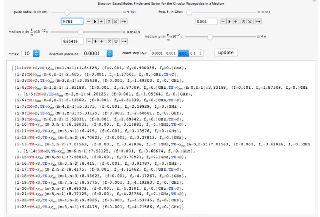
General view of our design while operating is given in Figure 1. It runs under the Mathematica CDF (Computable Document Format) player, which is a free-software downloadable from the Wolfram’s web page given in (Wolfram, 2017b). General properties of the CDF are given in (Guillermo and León, 2017; Hastings et al., 2016; Hong, 2016; Wellin, 2016; Wolfram, 2017b; Wolfram, 2017c; Wolfram Research, 2017) and some of the sample applications are available in (Al-Shamali, 2015; Beaulieu, 2012; Deshmukh, 2012; Hollingsworth and Narayanan, 2016; Jones, 2014; Kahle, 2014; Russel, 2013; Selinger, 2016; Tasgal and Band, 2015). To summarize, it can be coded to have a user console enabling real time computations. Moreover, once it is coded on Mathematica software, it can be easily converted to a CDF file which runs under the free CDF player without requiring any other software purchasing (Guillermo and León, 2017; Hastings et al., 2016; Hong, 2016; Wellin, 2016; Wolfram, 2017a; Wolfram, 2017b; Wolfram, 2017c; Wolfram Research, 2017).
Our Bisection-based algorithm involves two main stages. In the first stage, we use iterations by the desired scanning step (typically=0.01) to scan the related Bessel functions of first kind first and then its derivative to determine the critical points near the zeros for both roughly. These critical points are then instantaneously being processed by the conventional Bisection technique given in (Chapra and Canale, 2014; Hamming, 1987; Hoffman, 2001) to determine the related zeros in the second stage. In effect, we have very fast and accurate results since the iteration number for the desired accuracy level is very low (typically=5 iterations for the sensitivity set value=0.0001). Once these roots are found, they are unified and the conventional Bubble Sorting, which is normally known to be not much fast and practical (Arora et al, 2012; Astrachan, 2003; Cormen et al, 2009; Khairullah, 2013; Rohil and Manisha, 2014) is applied. Though, we have very fast and accurate modes in the correct order. Sorted and unified roots matrix is then re-scanned to determine the related mode type to be assigned for each. In effect, we have very fast and correctly ordered modes with the related cut-off and propagating wave frequency values. As seen in Figure 1, user console involves guide radius, operation frequency, relative permittivity and permeability values of the medium, maximum Bessel index value, Bisection precision value, count step value and an update button. When the update button is pushed, user selected values are entered.
Applications of the Bessel functions and their zeros to determine the modes of circular waveguides is being summarized in Chapter 2. Bisection method and our suggested algorithm regarding the numerical root finding based on the conventional Bisection method is being presented in Chapter 3 and their application to specific circular waveguide is being presented and discussed in Chapter 4.
CIRCULAR WAVEGUIDES
General properties of the 𝑇𝐸 and 𝑇𝑀 modes given in (Balanis, 1989; Cheng, 1989; Deniz, 2017; Kushwaha et al, 2014) can be summarized as follows:
TE Modes
The Transverse Electric to 𝑧, (𝑇𝐸𝑧) modes, can be derived by letting the vector potential 𝑨 and 𝑭 be equal to the followings:
𝑨 = 0 (2a)
𝑭 = 𝒂𝒛𝐹𝑧(𝜌, ∅, 𝑧) (2b)
from which we have ∇2𝐹
𝑧(𝜌, ∅, 𝑧) + 𝛽2𝐹𝑧(𝜌, ∅, 𝑧) = 0 (3a)
whose solution gives:
𝐹𝑧(𝜌, ∅, 𝑧) = [𝐴1𝐽𝑚(𝛽𝜌𝜌) + 𝐵1𝑌𝑚(𝛽𝜌𝜌)] × [𝐶2cos(𝑚∅) + 𝐷2sin(𝑚∅)]
× [𝐴3𝑒−𝑗𝛽𝑧𝑧+ 𝐵3𝑒𝑗𝛽𝑧𝑧]
(3b)
where
𝛽𝜌2+ 𝛽𝑧2= 𝛽2 (4)
and 𝐽𝑚&𝑌𝑚 are the Bessel functions of first and second kind respectively. Constants:
{𝐴1, 𝐵1, 𝐶2, 𝐷2, 𝐴3, 𝐵3, 𝑚, 𝛽𝜌, 𝛽𝑧} can be calculated by using the following boundary conditions:
𝐸∅(𝜌 = 𝑎, ∅, 𝑧) = 0 (5a)
𝐸𝑧(𝜌 = 𝑎, ∅, 𝑧) = 0 (5b)
from which we get
𝐹𝑧(𝜌, ∅, 𝑧) = 𝐴𝑚𝑛𝐽𝑚(𝛽𝜌𝜌) × [𝐶2cos(𝑚∅) + 𝐷2sin(𝑚∅)] × 𝐴3𝑒−𝑗𝛽𝑧𝑧 (6)
Then, the electric field component 𝐸∅+ can be calculated from
𝐸∅+(𝜌, ∅, 𝑧) =1 𝜀
𝜕𝐹𝑧+(𝜌,∅,𝑧)
𝜕𝜌 (7a)
and by applying the boundary condition for 𝐸∅+ in (5a), we get:
𝐸∅+(𝜌 = 𝑎, ∅, 𝑧) = 0 ⇒ 𝐽′𝑚(𝛽𝜌) = 0 ⇒ 𝛽𝜌= 𝜒𝑚𝑛′
where 𝜒′𝑚𝑛 represents the 𝑛th zero (𝑛 = 1, 2, 3, …) of the derivative of the Bessel function 𝐽𝑚(𝑥) of the first
kind of order 𝑚 (𝑚 = 0, 1, 2, 3, …). The smallest value of 𝜒′𝑚𝑛 corresponds to 𝜒′11= 1.8412 (𝑚 = 1, 𝑛 = 1).
Using (4) and (7b), 𝛽𝑧 of the 𝑚𝑛 mode can be written as follows:
(𝛽𝑧)𝑚𝑛 = { √𝛽2− 𝛽 𝜌2= √𝛽2− ( 𝜒′𝑚𝑛 𝑎 ) 2 , 𝛽 > 𝛽𝜌= 𝜒𝑚𝑛′ 𝑎 0, 𝛽 = 𝛽𝑐 = 𝛽𝜌= 𝜒′𝑚𝑛 𝑎 −𝑗√𝛽𝜌2− 𝛽2= 𝑗√( 𝜒′𝑚𝑛 𝑎 ) 2 − 𝛽2, 𝛽 < 𝛽 𝜌= 𝜒𝑚𝑛′ 𝑎 (8a) where Cut-off is defined when 𝛽𝑧(𝑚𝑛)= 0, namely:
𝛽𝑐 = 𝜔𝑐√𝜇𝜀 ⇒ (𝑓𝑐)𝑚𝑛 = 𝜒𝑚𝑛′
2𝜋𝑎√𝜇𝜀 (8b)
where (𝑓𝑐)𝑚𝑛 is the cut-off frequency above which the related 𝑇𝐸 mode propogates with the guide
wavelength: 𝜆𝑔=
2𝜋
(𝛽𝑧)𝑚𝑛 (8c)
TM Modes
Similarly, the Transverse Magnetic to 𝑧, (𝑇𝑀𝑧) modes, can be derived by letting the vector potential 𝑨 and 𝑭 be equal to the followings:
𝑭 = 0 (9a)
𝑨 = 𝒂𝒛𝐴𝑧(𝜌, ∅, 𝑧) (9b)
from which we have
∇2𝐴
𝑧(𝜌, ∅, 𝑧) + 𝛽2𝐴𝑧(𝜌, ∅, 𝑧) = 0 (10a)
whose solution gives:
𝐴𝑧(𝜌, ∅, 𝑧) = [𝐴1𝐽𝑚(𝛽𝜌𝜌) + 𝐵1𝑌𝑚(𝛽𝜌𝜌)] × [𝐶2cos(𝑚∅) + 𝐷2sin(𝑚∅)]
× [𝐴3𝑒−𝑗𝛽𝑧𝑧+ 𝐵3𝑒𝑗𝛽𝑧𝑧]
(10b) where
𝛽𝜌2+ 𝛽𝑧2= 𝛽2 (11)
and 𝐽𝑚&𝑌𝑚 are the Bessel functions of first and second kind respectively. Constants: {𝐴1, 𝐵1, 𝐶2, 𝐷2, 𝐴3, 𝐵3,
𝑚, 𝛽𝜌, 𝛽𝑧} can be calculated by using the following boundary conditions:
𝐸∅(𝜌 = 𝑎, ∅, 𝑧) = 0 (12a)
𝐸𝑧(𝜌 = 𝑎, ∅, 𝑧) = 0 (12b)
from which we get
𝐴𝑧+(𝜌, ∅, 𝑧) = 𝐵𝑚𝑛𝐽𝑚(𝛽𝜌𝜌) × [𝐶2cos(𝑚∅) + 𝐷2sin(𝑚∅)] × 𝐴3𝑒−𝑗𝛽𝑧𝑧 (13a)
Then, the electric field component 𝐸𝑧+ can be calculated from
𝐸𝑧+(𝜌, ∅, 𝑧) = −𝑗 1 𝜔𝜇𝜀( 𝜕2 𝜕𝜌2+ 𝛽 2) 𝐴 𝑧 +(𝜌, ∅, 𝑧) (13b)
and by applying the boundary condition in (12b) to (13b), we get 𝐸𝑧(𝜌 = 𝑎, ∅, 𝑧) = 0 ⇒ 𝐽𝑚(𝛽𝜌) = 0 ⇒ 𝛽𝜌=
𝜒𝑚𝑛
𝑎 (13c)
where 𝜒𝑚𝑛 represents the 𝑛th zero (𝑛 = 1, 2, 3, …) of the Bessel function 𝐽𝑚(𝑥) of the first kind of order 𝑚
(𝑚 = 0, 1, 2, 3, …). The smallest value of 𝜒𝑚𝑛 corresponds to 𝜒01= 2.4049 (𝑚 = 0, 𝑛 = 1).
Using (13c) and (11), 𝛽𝑧 of the 𝑚𝑛 mode can be written as follows:
(𝛽𝑧)𝑚𝑛= { √𝛽2− 𝛽 𝜌2= √𝛽2− ( 𝜒𝑚𝑛 𝑎 ) 2 , 𝛽 > 𝛽𝜌= 𝜒𝑚𝑛 𝑎 0, 𝛽 = 𝛽𝑐= 𝛽𝜌= 𝜒𝑚𝑛 𝑎 −𝑗√𝛽𝜌2− 𝛽2= 𝑗√( 𝜒𝑚𝑛 𝑎 ) 2 − 𝛽2, 𝛽 < 𝛽 𝜌= 𝜒𝑚𝑛 𝑎 (14)
where Cut-off is defined when 𝛽𝑧(𝑚𝑛)= 0, namely:
𝛽𝑐= 𝜔𝑐√𝜇𝜀 ⇒ (𝑓𝑐)𝑚𝑛= 𝜒𝑚𝑛
2𝜋𝑎√𝜇𝜀 (15)
where (𝑓𝑐)𝑚𝑛 is the cut-off frequency above which the related 𝑇𝑀 mode propogates with the guide
wavelength given in equation (8c). Since the cut-off frequencies of the 𝑇𝐸0𝑛 and 𝑇𝑀1𝑛 modes are
identical (𝜒0𝑛′ = 𝜒1𝑛), they are referred to also as degenerate modes.
DETERMINATION OF THE MODES The Bisection method
The conventional Bisection technique, based on the Intermediate Value Theorem, is also called as Binary-search method and it is applicable if 𝑓(𝜌) is a continuous function defined on the interval [𝑎 , 𝑏], with 𝑓(𝑎) and 𝑓(𝑏) of opposite sign as follows (Chapra and Canale, 2014; Hamming, 1987; Hoffman, 2001):
Theorem 1 (IVT): Assume 𝑓: 𝐼𝑅 → 𝐼𝑅 is a continuous function and there are two real numbers 𝑎 and 𝑏 such that 𝑓(𝑎) × 𝑓(𝑏) < 0. Then 𝑓(𝜌) has at least one zero between a and b.
The Intermediate Value Theorem implies that a number 𝑐 exists in (𝑎 , 𝑏) with 𝑓(𝑐) = 0. Although the procedure will work in most of the cases when there is more than one root in the interval (𝑎, 𝑏), we assume for simplicity that the root in this interval is unique for now. The method calls for a repeated halving (or bisecting) of sub-intervals of [𝑎, 𝑏] and, at each step, locating the half containing 𝑐 until the desired precision (=𝑝𝑟𝑒𝑐) is attained. To begin, set 𝑎1= 𝑎 and 𝑏1= 𝑏, and let 𝑝1 be the midpoint of [𝑎, 𝑏];
that is, 𝑐1= 𝑎1+ 𝑏1−𝑎1 2 = 𝑎1+𝑏1 2 (16)
Then the calculation involves the following procedures: i) If |𝑓(𝑐1)| ≤ 𝑝𝑟𝑒𝑐, then 𝑐 = 𝑐1, and we are done, root=𝑐.
ii) If 𝑓(𝑝1) ≠ 0, then 𝑓(𝑝1) has the same sign as either 𝑓(𝑎1) or 𝑓(𝑏1).
iii) If 𝑓(𝑝1) and 𝑓(𝑎1) have the same sign, 𝑝(𝑝1, 𝑏1). Set 𝑎2= 𝑐1 and 𝑏2= 𝑏1.
iv) If 𝑓(𝑝1) and 𝑓(𝑎1) have opposite signs, 𝑝(𝑎1, 𝑝1). Set 𝑎2= 𝑎1 and 𝑏2= 𝑐1.
v) Continue the same process to interval [𝑎2, 𝑏2] and reapply with 𝑟 iterations until |𝑓(𝑐 ← 𝑐𝑟)| ≤
𝑝𝑟𝑒𝑐, root=𝑐.
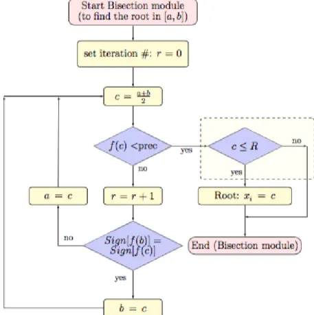
Flowchart of the Bisection algorithm used here is given in Figure 2. The dashed rectangle is our addition here to reject the roots found but out of the guide radius 𝑅. This modified Bisection module is used in our suggested algorithm whose flowchart is given in Figure 3 to find the root (which is guaranteed to exist by the IVT given above) in the determined [𝑎, 𝑏] interval instantaneously.
Figure 2. Flowchart of the Bisection algorithm to calculate the root of 𝑓(𝑥) between 𝑎&𝑏 by 𝑟 iterations. Our Suggestion
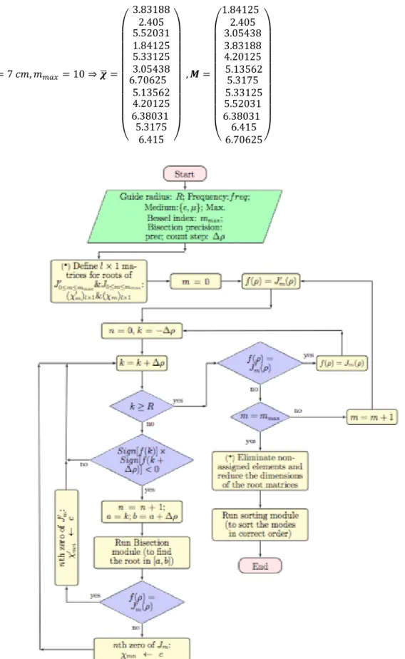
The flowchart of our suggestion is given in figure 3. User enters the following parameters: Guide radius (𝑅), frequency (𝑓𝑟𝑒𝑞), medium permittivity and permeability (𝜀, 𝜇), Bisection precision (𝑝𝑟𝑒𝑐) and, count step (∆𝜌). Bisection method discussed above operates in the determination of one zero between the end points [𝑎, 𝑏] where 𝑓(𝑎)&𝑓(𝑏) are in opposite signs satisfying the IVT as discussed. Since we study the functions with more than one zero, we suggest first to determine such critical points [𝑎𝑛, 𝑏𝑛] as follows:
[𝑎𝑛, 𝑏𝑛] = [𝑘, 𝑎𝑛+ ∆𝑚] (17a)
of the guide radius [0, 𝑅] in ∆𝜌 steps. Here we determine the critical point pairs {𝑎𝑛, 𝑏𝑛} obeying the IVT
as follows:
𝑆𝑖𝑔𝑛[𝑓(𝑎𝑛)] × 𝑆𝑖𝑔𝑛[𝑓(𝑏𝑛)] ≤ 0 (17b)
By this suggestion, the application of the Bisection method can be started within very close critical point pairs {𝑎𝑛, 𝑏𝑛}. So, less iteration steps are needed in the application of the Bisection method. Since
the 𝑛th zeros of 𝐽𝑚′ (𝑥)&𝐽𝑚(𝑥) are searched to determine the modes 𝜒𝑚𝑛′ &𝜒𝑚𝑛 in each application of the
Bisection method, the user initially enters the maximum value of 𝑚 (=𝑚𝑚𝑎𝑥), hence we have: 𝑚 =
0,1,2, … , 𝑚𝑚𝑎𝑥. Once all the parameters are been entered and activated by the update button by the user,
𝜒𝑚′ 𝑙×1matrix for the roots of 𝐽𝑚′(𝜌) and similarly, 𝜒𝑚 𝑙×1 matrix for the roots of 𝐽𝑚(𝜌) are defined in order
that final results for the roots can be assigned to these matrices. So, starting from 𝑘 = 0 and 𝑓(𝜌) = 𝐽𝑚=0′ (𝜌), all the roots are found and assigned to the related elements of matrix 𝜒0′𝑙×1. When 𝑘 reaches 𝑅, it
is complete and it repeats for 𝑓(𝜌) = 𝐽𝑚=0(𝜌) from 𝑘 = 0 up to 𝑘 = 𝑅 and all the roots are found and
assigned to the related elements of matrix 𝜒0𝑙×1. Then the same procedure continues for the next 𝑚 value with 𝑚 = 1 and repeats up to 𝑚 = 𝑚𝑚𝑎𝑥 to find and assign all the roots to the related matrices in the
following order: {𝝌𝑚′ = (𝜒𝑚1′ 𝜒𝑚2′ … 𝜒𝑚𝑛′ … 𝜒𝑚′𝑚𝑎𝑥𝑙) 𝑇 , 𝝌𝑚= (𝜒𝑚1 𝜒𝑚2… 𝜒𝑚𝑛… 𝜒𝑚𝑚𝑎𝑥𝑙) 𝑇} ,𝑚 = 0,1,2, … , 𝑚𝑚𝑎𝑥 𝑛 = 1,2,3, … , 𝑙 (18) Note that 𝑙 is a relatively big number (typically 50 or more) regarding the maximum root number in 0 ≤ 𝜌 ≤ 𝑅 and 0 ≤ 𝑚 ≤ 𝑚𝑚𝑎𝑥, which is not known at the beginning and the blocks marked by (*) are not
necessary if any matrix predefinition is not required by the programming language in use or by the preference of the programmer. Deletion of the non-assigned elements to reduce the matrices at the end of this module is also optional. The outputs at the end of this module for a relatively small guide radius (𝑅 = 7 𝑐𝑚, 𝑚𝑚𝑎𝑥= 10) is given as an example as follows:
𝑅 = 7 𝑐𝑚, 𝑚𝑚𝑎𝑥= 10 ⇒ { 𝑚 = 0 ⇒ 𝝌0′ = (3.83188), 𝝌0= (2.405 5.52031)𝑇 𝑚 = 1 ⇒ 𝝌1′ = (1.84125 5.33125)𝑇, 𝝌1= (3.83188) 𝑚 = 2 ⇒ 𝝌2′ = (3.05438 6.70625)𝑇, 𝝌2= (5.13562) 𝑚 = 3 ⇒ 𝝌3′ = (4.20125), 𝝌3= (6.38031) 𝑚 = 4 ⇒ 𝝌4′ = (5.3175), 𝝌4= 𝜙 𝑚 = 5 ⇒ 𝝌5′ = (6.415), 𝝌4= 𝜙 (19)
Note that for 5 < 𝑚 ≤ 𝑚𝑚𝑎𝑥= 10, 𝜒𝑚 or 𝜒𝑚′ exceeds 𝑅 = 7 𝑐𝑚.
Sorting Module
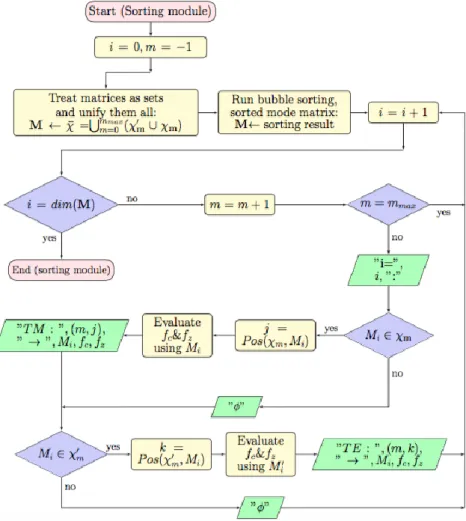
Flow chart algorithm for our sorting module is given in figure 4. We prefer the conventional Bubble sorting given in (Arora et al, 2012; Astrachan, 2003; Cormen et al, 2009; Khairullah, 2013; Rohil and Manisha, 2014). For small guide radius value given above we have the following operations:
𝝌
̅ =∪𝑚=0𝑚𝑚𝑎𝑥(𝝌 𝑚 ′ ∪ 𝝌
𝑅 = 7 𝑐𝑚, 𝑚𝑚𝑎𝑥 = 10 ⇒ 𝝌̅ = ( 3.83188 2.405 5.52031 1.84125 5.33125 3.05438 6.70625 5.13562 4.20125 6.38031 5.3175 6.415 ) , 𝑴 = ( 1.84125 2.405 3.05438 3.83188 4.20125 5.13562 5.3175 5.33125 5.52031 6.38031 6.415 6.70625 ) (20b)
Figure 3. Flowchart of the suggested algorithm to calculate and sort the zeros of 𝐽𝜈′(𝜌) and 𝐽𝜈(𝜌) in the
Unsorted roots (both for 𝝌𝑚′ and 𝝌𝑚) are assigned to column matrix 𝝌̅ and they are sorted in the
column matrix 𝑴. Indice 𝑖 scans from 0 up to 𝑑𝑖𝑚(𝑀) and each time indice 𝑚 scans from 0 up to 𝑚𝑚𝑎𝑥
and 𝑀𝑖∈ 𝝌𝑚′ is checked. If it is true, row number of element 𝑀𝑖 in 𝝌𝑚′ is assigned as indice 𝑛 of the 𝜒𝑚𝑛′ .
If it is false, 𝑀𝑖∈ 𝝌𝑚 is checked and if it is true, row number of element 𝑀𝑖 in 𝝌𝑚 is assigned as indice 𝑛
of the 𝜒𝑚𝑛. Note that 𝜒01′ = 𝜒11= 3.83188 in our simplified illustration. It is due to the fact that (Balanis,
1989; Beattie, 1958; Cheng, 1989; Deniz, 2016; Deniz, 2017; Kushwaha et al, 2014; Sekeljic, 2010):
𝜒0𝑛′ = 𝜒1𝑛 (21)
where the related TM and TE modes are common. Such common modes are also detected by the sequential checking in our design.
Figure 4. Flowchart of the sorting module RESULTS AND CONCLUSION
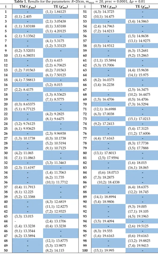
Results for relatively large parameters are given in Table 1. They are in agreement with the results given in (Balanis, 1989; Beattie, 1958; Cheng, 1989; Deniz, 2016; Deniz, 2017; Kushwaha et al, 2014; Sekeljic, 2010) and in the correct order as in (Beattie, 1958), where the first 700 zeros are listed in the correct order as a reference table. Note that results in (Beattie, 1958) with as much as first 700 modes are sorted by the inspection of the author, obviously requiring a great effort without using any sorting algorithm for quick access for practical applications. Although we use here a slow and impractical Bubble sorting as discussed in (Arora et al, 2012; Astrachan, 2003; Cormen et al, 2009; Khairullah, 2013; Rohil and Manisha, 2014), we have very fast and accurate results in the correct mode orders as aimed here. It is enabled by the use of the suggested algorithm running under the free Mathematica CDF player
which offers a real time computation with the user console. Our simplified illustration for selected parameters 𝑅 = 7 𝑐𝑚, 𝑚𝑚𝑎𝑥 = 10 given in Section 3.3 can be followed and verified from Table 1 between
the index numbers 𝑖 = 1 and 𝑖 = 12.
It is obvious that as the selected parameter 𝑚𝑚𝑎𝑥 increases, the maximum 𝑚 value of 𝝌𝒎𝒏 and 𝝌𝒎𝒏′ to
be found and sorted increases and similarly, as the parameter 𝑅 increases maximum 𝑛 value of 𝝌𝒎𝒏 and
𝝌𝒎𝒏′ to be found and sorted increases, too. However, as seen in our algorithm in Figure 3, both
parameters are checked and Bisection method is applied provided that 𝑘 < 𝑅 and 𝑚 < 𝑚𝑚𝑎𝑥 holds. All
the first 𝑛′ → 𝑛th roots of 𝐽𝑚′ (𝜌) are first determined until 𝑘 = 𝑅 is reached then 𝑘 → 0 and all the first 𝑛th
roots of 𝐽𝑚(𝜌) are then obtained until 𝑘 = 𝑅 is reached again by the Bisection method. When both are
completed, 𝑚 is increased by one and it repeats again. Then it sequentially continues until 𝑚 = 𝑚𝑚𝑎𝑥 is
reached (𝑚 = 𝑚𝑚𝑎𝑥 is included). So, our design finds the roots in the following orders:
𝑚 = 0: 𝜒01′ , 𝜒02′ , 𝜒03′ , … 𝜒0𝑛′ ′ , 𝜒 01, 𝜒02, 𝜒03, … 𝜒0𝑛, 𝑚 = 1: 𝜒11′ , 𝜒12′ , 𝜒13′ , … 𝜒1𝑛′ , 𝜒11, 𝜒12, 𝜒13, … 𝜒1𝑛, 𝑚 = 2: 𝜒21′ , 𝜒22′ , 𝜒23′ , … 𝜒2𝑛′ ′ , 𝜒21, 𝜒22, 𝜒23, … 𝜒2𝑛 ⋮ 𝑚 = 𝑚𝑚𝑎𝑥: 𝜒𝑚′𝑚𝑎𝑥1, 𝜒𝑚′𝑚𝑎𝑥2, 𝜒𝑚′𝑚𝑎𝑥3, … 𝜒𝑚𝑚𝑎𝑥𝑛′ ′ , 𝜒 𝑚𝑚𝑎𝑥1, 𝜒𝑚𝑚𝑎𝑥2, 𝜒𝑚𝑚𝑎𝑥3, … 𝜒𝑚𝑚𝑎𝑥𝑛 (22)
Each root is assigned to the related matrix as given in (18). Note that maximum root number of 𝐽𝑚′ (𝜌)
is denoted by 𝑛′ but maximum root number of 𝐽𝑚(𝜌) by 𝑛 here since they may not be equal, though both
are counted by the same dummy index 𝑛 and when 𝑘 = 𝑅 is reached for either one (for 𝐽𝑚′ (𝜌) or 𝐽𝑚(𝜌) in
the related loop), corresponding 𝑛 value for that loop determines the maximum root numbers (say, 𝑛 → 𝑛′ for 𝐽𝑚′(𝜌) and 𝑛 for 𝐽𝑚(𝜌)). Also note that predefined dimensions of matrices (𝝌𝑚′ and 𝝌𝑚) are
large when compared to 𝑛 and 𝑛’ values, namely: 𝑛 ≤ 𝑙 and 𝑛′ ≤ 𝑙.
As the radius (𝑅) increases, zeros of Bessel functions and their derivatives get closer so, choosing small count step values (∆𝜌) prohibits a missing root. On the other hand, too small count step values cause great iteration numbers to scan, which means a decrease in the calculation speed, for small 𝑅 values. For this reason, parameter: “count step values (∆𝜌)” is introduced in the user console as seen in Figure 1. For large 𝑅 values, greater ∆𝜌 parameter to scan can be chosen to avoid a missing root by the user. Similarly, the “Bisection precision” parameter is essential as seen in Figure 1 and in Figure 2. Bisection method sequentially repeats until 𝑝𝑟𝑒𝑐 < 𝑓(𝑐) and this means that smaller 𝑝𝑟𝑒𝑐 parameters cause greater iteration numbers and hence a reduction in speed. Note that, in order to detect and find a root (whatever the precision parameter is), ∆𝜌 parameter should not cause a missing root by the IVT given in Theorem 1 above. Moreover, as the radius increases, choosing lower precision values are advantageous since then the higher order roots get closer. Optimum values of ∆𝜌 and 𝑝𝑟𝑒𝑐 values for user selections are introduced in the user console.
Our sorting module whose flowchart is given in Figure 4 also increases the calculation speed since the unified sorted matrix 𝑴 is used to compare with the related 𝝌𝑚′ and 𝝌𝑚 matrices to determine their
positions (and hence their correct orders). Even though a relatively impractical and slow sorting method (the Bubble sorting) is used here, in effect, related modes and propagating wave frequencies are found accurately and in the correct order with a very fast and instantaneous calculation.
Table 1. Results for the parameters: 𝑅=20cm, 𝑚𝑚𝑎𝑥= 20, 𝑝𝑟𝑒𝑐 = 0.0001, ∆𝜌 = 0.01 i TM ( 𝝌𝒎𝒏) TE (𝝌𝒎𝒏′ ) i TM ( 𝝌𝒎𝒏) TE (𝝌𝒎𝒏′ ) 1 - (1,1): 1.84125 51 (4,3): 14.3725 - 2 (0,1): 2.405 - 52 (10,1): 14.475 - 3 - (2,1): 3.05438 53 - (3,4): 14.5863 4 (1,1): 3.83188 (0,1): 3.83188 54 (2,4): 14.7963 - 5 - (3,1): 4.20125 55 (7,2): 14.8213 - 6 (2,1): 5.13562 - 56 - (1,5): 14.8638 7 - (4,1): 5.3175 57 - (13,1): 14.9275 8 - (1,2): 5.33125 58 (0,5): 14.9312 - 9 (0,2): 5.52031 - 59 - (6,3): 15.2681 10 (3,1): 6.38031 60 - (9,2): 15.2863 11 - (5,1): 6.415 61 (11,1): 15.5894 - 12 - (2,2): 6.70625 62 (5,3): 15.7006 - 13 (1,2): 7.01563 (0,2): 7.01563 63 - (4,4): 15.9638 14 - (6,1): 7.50125 64 - (14,1): 15.975 15 (4,1): 7.58813 - 65 (8,2): 16.0375 - 16 - (3,2): 8.015 66 (3,4): 16.2238 - 17 (2,2): 8.4175 - 67 - (2,5): 16.3475 18 - (1,3): 8.53625 68 - (10,2): 16.4475 19 - (7,1): 8.5775 69 (1,5): 16.4706 (0,5): 16.4706 20 (0,3): 8.65375 - 70 - (7,3): 16.5294 21 (5,1): 8.77125 - 71 (12,1): 16.6988 - 22 - (4,2): 9.2825 72 (6,3): 17.0038 - 23 - (8,1): 9.6475 73 - (15,1): 17.0213 24 (3,2): 9.76125 - 74 (9,2): 17.2413 - 25 (6,1): 9.93625 - 75 - (5,4): 17.3125 26 - (2,3): 9.96938 76 - (11,2): 17.6006 27 (1,3): 10.1738 (0,3): 10.1738 77 (4,4): 17.6163 - 28 - (5,2): 10.5194 78 - (8,3): 17.7738 29 - (9,1): 10.7125 79 - (3,5): 17.7888 30 (4,2): 11.065 - 80 (13,1): 17.8013 - 31 (7,1): 11.0863 - 81 (2,5): 17.9594 - 32 - (3,3): 11.3463 82 - (1,6): 18.015 33 (2,3): 11.6197 - 83 - (16,1): 18.065 34 - (1,4): 11.7063 84 (0,6): 18.0713 - 35 - (6,2): 11.735 85 (7,3): 18.2875 - 36 - (10,1): 11.7712 86 (10,2): 18.4338 - 37 (0,4): 11.7913 - 87 - (6,4): 18.6375 38 (8,1): 12.225 - 88 - (12,2): 18.745 39 (5,2): 12.3388 - 89 (14,1): 18.8994 - 40 - (4,3): 12.6819 90 (5,4): 18.9806 - 41 - (11,1): 12.8275 91 - (9,3): 19.005 42 - (7,2): 12.9325 92 - (17,1): 19.105 43 (3,3): 13.015 - 93 - (4,5): 19.1963 44 - (2,4): 13.1706 94 (3,5): 19.4094 - 45 (1,4): 13.3238 (0,4): 13.3238 95 - (2,6): 19.5125 46 (9,1): 13.3544 - 96 (8,3): 19.555 - 47 (6,2): 13.5894 - 97 (1,6): 19.6163 (0,6): 19.6163 48 - (12,1): 13.8775 98 - (13,2): 19.8825 49 - (5,3): 13.9875 99 - (7,4): 19.9413 50 - (8,2): 14.115 100 (15,1): 19.995 - REFERENCES
Abramowitz, A., Stegun, I.A., 1965, Handbook of Mathematical Functions, with Formulas, Graphs, and Mathematical Tables, 3rd Printing with Corrections, Vol. 55 of NBS Applied Mathematics Series, Superintendent of Documents, US Government Printing Office, Washington DC, pp. 355—479.
Abuelma’atti, M. T., 1999, “Trigonometric Approximations for Some Bessel functions”, Active and Passive Elec. Comp., Vol. 22, pp. 75-85.
Al-Shamali, F., 2015, “Interactive CDF Diagrams in Introductory Physics Course”, Proceedings of 20th International Conference on Multimedia in Physics Teaching and Learning, LMU Munich, p. 77. Arfken, H.J., Weber, G.B., 2005, Mathematical Methods for Physicists (6th ed.), Elsevier Academic Press, pp.
675—686.
Arora, N., Kumar, S., Tamta, V.K., 2012, “A Novel Sorting Algorithm and Comparison with Bubble Sort and Insertion Sort”, International Journal of Computer Applications, Vol. 45(1), pp. 31-32.
Astrachan, O., 2003, “Bubble Sort: An Archaeological Algorithmic Analysis”, SIGCSE '03 Proceedings of the 34th SIGCSE Technical Symposium on Computer Science Education, NY, pp. 1-5.
Balanis, C., 1989, Advanced Engineering Electromagnetics (2nd ed.), Wiley, NY, pp. 483—500.
Beattie, C. L., 1958, “Table of First 700 Zeros of Bessel Functions”—Jl(x) and Jl’(x), Bell System Technical
Journal, Vol. 37, pp. 689-697.
Beaulieu, J.R., 2012, A Dynamic, Interactive Approach to Learning Engineering and Mathematics, MSc. Thesis in Mechanical Eng., Virginia Polytechnic Institute and State University, Blacksburg, VA. Bell, W.W., 1968, Special Functions for Scientists and Engineers, D. Van Nostrand Compant Ltd., London,
pp. 92-110.
Blachman, N. M., Mousavinezhad, S. H., 1986, “Trigonometric Approximations for Bessel functions”, EEE Transactions on Aerospace and Electronic Systems, Vol. AES-22(1), pp.2-7.
Boas, L.M., 2006, Mathematical Methods in the Physical Sciences (3rd ed.), Wiley, NY, pp. 587—606.
Chapra, S., Canale, R., 2014, Numerical Methods for Engineers (7th ed.), WCB/McGraw-Hill, NY, pp.
148-154.
Cheng, D. K., 1989, Field and Wave Electromagnetics (2nd ed.), Addison-Wesley, London, pp., 562-572.
Cormen, T. H., Leiserson, C. E., Rivest, R. L., Stein, C., 2009, Introduction to Algorithms (3rd ed.), MIT
Press, USA, p. 40.
Deniz, C., 2016, “A Secant Based Roots Finding Algorithm Design and its Applications to Circular Waveguides”, IOSR Journal of Electrical and Electronics Engineering, Vol. 11(6), Ver. III, pp. 84-91.
Deniz, C., 2017, “A Newton Raphson Based Roots Finding Algorithm Design and its Applications to Circular Waveguides”, El-Cezeri Journal of Science and Engineering, Vol. 4(1), pp. 32-45.
Deshmukh, S., 2012, Illustration of Fundamentals of Vibrations Using Computable Document Format, MSc. Thesis in Mechanical Eng., The University of Texas At Arlington.
Guillermo, J., León, S., 2017, Mathematica Beyond Mathematics: The Wolfram Language in the Real World, CRC press- Taylor & Francis group, NY.
Hamming, R. W., 1987, Numerical Methods for Scientists and Engineers (2nd Revised ed., Dover Books on Mathematics), Dover Publications, NY, pp. 68-72.
Harrison, J., 2009, “Fast and Accurate Bessel Function Computation”, Computer Arithmetic-proc. of 19th
IEEE symp. on Computer Arithmetic, Portland-Oregon, pp. 104-113.
Hastings, C., Mischo, K., Morrison, M., 2016, Hands-On Start to Wolfram Mathematica: And Programming with the Wolfram Language, 2nd ed., Wolfram Media Inc., Canada.
Hoffman, J.D., 2001, Numerical Methods for Engineers and Scientists, (2nd ed.), Marcel Dekkel, NY-Basel, pp.
141-154.
Hollingsworth, M.L. and Narayanan, N.H., 2016, “Building a Better eTextbook”, Bulletin of the IEEE Technical Committee on Learning Technology, Vol. 18, No. 2/3, pp. 14-17.
Hong, W., 2016, Art of Mathematics, Dorrance Publishing, Pittsburg, pp. 165—166.
Jones, J., 2014, The Technical and Social History of Software Engineering, Pearson, NJ, pp. 201-203.
Kahle, D., 2014, “Animating Statistics: A New Kind of Applet for Exploring Probability Distributions”, Journal of Statistics Education, Vol. 22, No. 2, pp. 1-21.
Khairullah, Md., 2013, “Enhancing Worst Sorting Algorithms”, International Journal of Advanced Science and Technology, Vol. 56, pp. 13-26.
Korenev, B.G., 2002, Bessel Functions and Their Applications, Taylor and Francis, NY.
Kushwaha, R. K., Srivastava, S., Chaursiya, V., 2014, “A Novel Approach to Analyze a Circular Waveguide in Air and Dielectric Medium”, SOP Transactions on Wireless Communications, Vol. 1, No. 2, pp. 1-18.
Luke, Y. L., 1975, Approximation of Special Functions, Academic Press, NY.
Millane R. P., Eads, J. L., 2003, “Polynomial Approximations to Bessel Functions”, IEEE Transactions on Antennas and Propagation, Vol. 51(6), pp. 1398-1400.
Newman, J. N., 1984, “Approximations for the Bessel and Struve functions”, Mathematics of Computation, Vol. 43(168), pp. 551-556.
Richards, D., 2002, Advanced Mathematical Methods with Maple, Cambridge University Press, UK, pp. 325-331.
Rohil, H., Manisha, 2014, “Run Time Bubble Sort–An enhancement of Bubble Sort”, International Journal of Computer Trends and Technology (IJCTT), Vol. 14(1), pp. 36-38.
Russel, D. A., 2013, “Creating İnteractive Acoustics Animations using Mathematica's Computable Document Format”, Proceedings of Meetings on Acoustics, Vol. 19, 025006.
Sekeljic, N., 2010, “Asymptotic Expansion of Bessel Functions; Applications to Electromagnetics”, Dynamics at the Horsetooth, Focused Issue: Asymptotics and Perturbations, Vol. 2A, pp. 1-11.
Selinger, J. V., 2016, Introduction to the Theory of Soft Matter from İdeal Gases to Liquid Crystals, Springer, OH-USA.
Tasgal, R. S., Band, Y.B., 2015, “Sound Waves and Modulational İnstabilities on Continuous-Wave Solutions in Spinor Bose-Einstein Condensates”, Physical Review, A 91, 013615, pp. 1-15.
Waldron, R.A., 1981, “Formulas for Computation of Approximate Values of Some Bessel Functions”, Proceedings of the IEEE, Vol. 69, pp. 1686-1588.
Watson, G. N., 1995, A Treatise on the Theory of Bessel Functions, (2nd ed.), Cambridge University Press,
NY.
Wellin, P., 2016, Essentials of Programming in Mathematica, 1st ed., Cambridge, Cambridge University Press, pp. 449-493.
Wolfram, S., 2003, The Mathematica Book (5th ed.), Wolfram Media Inc., 5th edition, USA, pp. 29-35 & pp.
102-110.
Wolfram, S., 2017a, Wolfram Documentation Center, BesselJ,
http://reference.wolfram.com/mathematica/ref/BesselJ.html (accessed in 22 February 2017). Wolfram, S., 2017b, Wolfram CDF player, https://www.wolfram.com/cdf-player/ (accessed in 22 February
2017).
Wolfram, S., 2017c, Computable Document Format, http://www.wolfram.com/events/siam-2016/files/CDF-4.pdf (accessed in 22 February 2017).