e-ISSN: 2 ISSN: 25 R Abstrac this fam baseline hazard discusse numeric Keywor Özet. S üstel da çalışılm elde edi kareler modelle Anahtar 1. INTR Distribut many sta distribut paramete function where f the skew 2587-246X 587-2680 İsmail Kına 1Departm 2 Dep Received: 11.10. ct. Recently,
mily with exp e distribution rate and surv ed. Simulatio cal example is rds: Distributio on zamanlard ğılım durumu mıştır. APT-Pa ilmiştir. En ço ortalamaların emedeki kullan r Kelimeler: D RODUCTIO tion theory i atistical distr tion function er l to the n of Z is of f and F a w-normal dist
Cu
APT-Pa
acı1 ,Coşk
ment of Actua partment of S . 2018; Accepte the APT-fami ponential distr in APT-famil vival function n study is al s given to illus on family, EstAPT
da, APT-dağıl unu detaylı bir areto dağılımın ok olabilirlik v nı elde edeb nılabilirliğini Dağılımlar ail ON s one of the ributions are ns. Azzalini e normal dist fare the standa tribution is re
umhu
areto Distr
kun Kuş
2 arial Science Statistics, Se ed: 19.10.2018ily has been i ribution is ex ly. Several pro ns are derive
lso performed strate the capa
timation, Pare
T-Pareto D
lım ailesi adın r şekilde ele al na ilişkin mom ve en küçük k bilmek için s göstermek am esi, Tahmin, P most import e introduced i [1] introdu tribution. Let ( ; ) f z l = ard normal d educed standuriyet
ribution a
,Kadir Ka
es, Selçuk Un elçuk Univers introduced as xamined in d roperties of th ed. The maxi d to get the ability of APT eto distributionDağılımı
nda yeni bir d lınmıştır. Bu m mentler, hazar kareler yöntem simülasyon ç macıyla gerçek Pareto dağılım tant areas of d by includin uced the sk t Z be the ( ) ( 2f l = z F density and d dard normal
t Scien
CSJ
Cumhuriyetand its Pr
arakaya
2* niversity, 422 sity, 42250, K http://dx.d a new family details. In this he APT-Pareto mum likeliho bias and me T-Pareto distrib n, Simulationve Özellik
dağılım ailesi makalede, AP rd fonksiyonu mleri tartışılmı çalışması yap k bir veri uygu mı, Simülasyon f statistics. In ng an extra p kew normal skew-norma ), , lz z istribution fu distributionnce Jo
Sci. J., Vol.40roperties
,Yunus Ak
250, Konya, Konya, TURK doi.org/10.1777 y of distributio s paper, Paret o distribution ood and least ean square er bution for mo .kleri
tanıtılmıştır. B T-dağılım aile u, yaşam fonk ıştır. Tahmin pılmıştır. AP ulaması yapılm nn the last two parameter to distribution al random va unction, resp for 0.
ourna
0-2 (2019) 378kdoğan
2 TURKEY RKEY 76/csj.469493 ons. A specia to is conside such as the m t square meth rrors of estim odelling real da Bu dağılım a esinde Pareto ksiyonu gibi öz edicilerin yan PT-Pareto dağ mıştır. o decades, th o an existing n by adding ariable, then t pectively. It ial
8-387 al case of ered as a moments, hods are mates. A ata. ilesi için dağılımı zellikleri n ve hata ğılımınınhere are too g family of g an extra
the density
Mudholkar and Srivastava [2] proposed a method to include an extra parameter to a two-parameter Weibull distribution. If a random variable Z has distribution function F z( ), then (F z( ))q
(q >0) is also distribution function and it is called exponentiated family, where F z( ), is baseline distribution. Mudholkar and Srivastava [2] considered F z( )=
(
1 exp- (-z/s)a)
as a baseline distribution and they get the distribution with cdf( )= -
(
1 exp(- /s)a)
qF z z
and called it as exponentiated-Weibull family, where q is an extra parameter. Some exponentiated distributions have been introduced by several authors, see for example Gupta et al. [3], Gupta and Kundu [4] and etc.
Marshall and Olkin [5] proposed another method to introduce an additional parameter to any distribution function as follows. Let Z is a random variable with cdf F and density f , then
( ) ( ) ( )( ( )) {1 1 1 }2 a a = - - -f z g z F z
is also pdf of a random variable, where a is an extra parameter. Marshall and Olkin [5] cosidered exponential and Weibull distribution for baseline distribution f z( ).
Eugene et al. [6] proposed the beta generated method which is defined as follows: Let Z is a random variable with cdf F , then
( ) ( ) ( ) ( ) ( ) ( ) 1 1 0 1 b , a a b a b -G + = -G G
ò
F z G z t t dtis a distribution function as well, where (a b, ) 2 +
is an extra parameter vector.
Alzaatreh et al. [7] introduced a new method for generating families of continuous distributions called T-X family using same idea of Eugene et al. [6]
Mahdavi and Kundu [8] introduced an extra parameter to a family of distributions functions to bring more flexibility to the given family. This new method is called a -power transformation (APT) method. The proposed APT method is very easy to use, hence it can be used extensively for the data modelling purposes. The pdf and cdf of APT-family are given, respectively, by
( ) ( ) ( ) ( ) ( ) ( ) log 1 , 1 , 1 a a a a a -ìï ¹ ï = íï = ïî F x A APT f x I x f x f x (1) and ( ) ( ) ( ) ( ) 1 1 , 1 , 1, a a a a -ìï ¹ ï = íï = ïî F x A APT I x F x F x (2) where a > is an extra parameter and 0 IA( )x is indicator function on set A which is domain of baseline distribution. Mahdavi and Kundu [8] applied the a -power transformation to exponential
distribution.
An extra parameter supplies more flexibility to a class of distribution functions and it can be very useful for the data analysis. It should be point out that the adding extra parameter caused the estimation problem, but it can be solved by numerical methods. R and Matlab have several numerical algorithms for this job.
In this paper, a -power transformation is applied to Pareto distribution. In Section 2, moments, hazard rate and survival functions are given. The maximum likelihood and least square methods are discussed in Section 3. In Section 4, a simulation study is also performed to observe the performance of the estimates. A numerical example with the real data is given to illustrate the flexibility of APT-Pareto distribution for modelling real data in Section 5.
2. a -POWER PARETO DISTRIBUTION
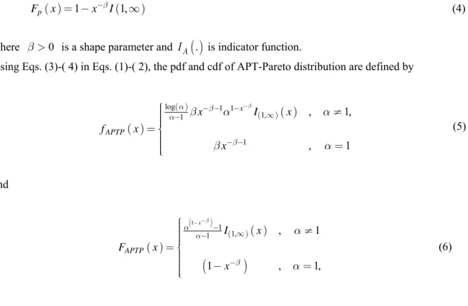
In this paper, Pareto distribution is considered. The pdf and cdf of the Pareto distribution are given, respectively, by ( )=b - -b 1 (1,¥) p f x x I (3) and ( )= -1 -b (1,¥) p F x x I (4)
where b > is a shape parameter and 0 IA
( )
. is indicator function.Using Eqs. (3)-( 4) in Eqs. (1)-( 2), the pdf and cdf of APT-Pareto distribution are defined by
(5) and ( ) ( ) ( )( )
(
)
1 1 1, 1 , 1 1 , 1, b a a b a a -¥ -ìïï ¹ ïïï = í ïï ï - = ïïî x APTP I x F x x (6)respectively. The random variable X is said to have a two-parameter APT-Pareto distribution and it is denoted by APTP( , )a b .
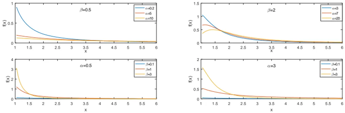
Fig. 1 presents the plots pdf of APTP( , )a b for some choices of a and b .
( ) ( ) ( )( ) log 1 1 1, 1 1 , 1, , 1 b a b a b b a a b a -- -- -¥ -ìï ¹ ïï ï = í ïï = ïïî x APTP x I x f x x
Figure 1. Pdf of APTP distribution for some choices of a and b
In the rest of paper, the case a ¹ is only considered. The survival function and the hazard rate 1 function for APTP distribution are given in the following forms
( ) (1 ) 1 b a a a -= -x APTP S x and ( ) ( ) ( ) 1 1 1 log , b b b a b a a a -- -- -= -x APTP x x h x
respectively. Fig. 2 presents the plots the hazard rate function of APTP( , )a b for some choices of a
and .b
Figure 2. Hazard rate function of APTP distribution for some choices of a and b The r th moment of APTP distribution is obtained by
( )
( ) ( ) ( ) ( ) ( ) ( )(
)
(
( )(
( ))
)
( )( )( )( ) ( )(
)
(
(
( ))
( ( ) ))
( )( )( )( ) 2 2 1 2 2 1 1 1 0 2 2 3 2 2 3 2 2 log 1 log log 1 1 . 1 ! 1 log 2 , , log 2 3 1log , , log log 2
2 3 1 b b b b b b b b b b b b b a b a a a a ab a b a b b a b b a b a b b a a b b b b a b -¥ - - -¥ = - + - + - + -= -æ ö÷ ç = - - ççè - + ÷÷ø -= - - - -- -- - -
-ò
å
r r r x i i i r r r r E X x x dx i r i a r WhittakerM r r r a WhittakerM r r r r , 1 1.5 2 2 .5 3 3 .5 4 4 .5 5 5 .5 6 x 0 0 .5 1 f( x ) =0.5 =0.2 =5 =10 1 1 .5 2 2 .5 3 3 .5 4 4 .5 5 5.5 6 x 0 0 .5 1 1 .5 f( x ) =2 =3 =7 =20 1 1.5 2 2 .5 3 3 .5 4 4 .5 5 5 .5 6 x 0 1 2 3 4 f( x ) =0.5 =0.1 =1 =3 1 1 .5 2 2 .5 3 3 .5 4 4 .5 5 5.5 6 x 0 0 .5 1 1 .5 2 f( x ) =3 =0.1 =1 =3 1 1 .5 2 2 .5 3 3 .5 4 4 .5 5 5 .5 6 x 0 0 .5 1 1 .5 h (x ) =2 =2 =5 =10 1 1 .5 2 2 .5 3 3 .5 4 4 .5 5 5 .5 6 x 0 0 .5 1 1 .5 h (x ) =0.5 =0.1 =2 =5 1 1 .5 2 2 .5 3 3 .5 4 4 .5 5 5 .5 6 x 0 0 .2 0 .4 0 .6 h (x ) =2 =0.2 =0.5 =0.8 1 1 .5 2 2 .5 3 3 .5 4 4 .5 5 5 .5 6 x 0 2 4 6 h (x ) =2 =1 =4 =7where the WhittakerM( , ,a b c ) is a Whittaker function and it can be easily calculated by Maple or Matlab. It should be noted that r th moments works for only 3
2
b > r . This restriction has been observed in simulation study. It is not proved here.
Moment generating function of APTP distribution is given by
( ) ( ) ( ) ( ) ( ) ( )( ( )) ( ( ) ) 1 1 1 1 0 log exp 1 log log 1 , 1 ! b b b a b a a a ba a b a -¥ - - -¥ + = = -- - G - + -=
-ò
å
x X i i i M t tx x dx t i t i where G a b is the incomplete gamma function. ( , )3. ESTIMATION
3.1. Maximum-Likelihood Method
Let X1,X2, , Xn be a random sample from APTP( , )a b , then log-likelihood function is given by
( ) ( ) ( ) ( ) ( ) ( )
1 1
log
, log log 1 log log .
1 b a a b b b a a = = æ ö æ ö÷ ç ÷ ç ç ÷ = çèç - ÷÷ø+ - + +ç - ÷÷÷ çè ø
å
å
n n i i i i n n x n xThe likelihood equations are found to be
( ) ( ) ( ) ( ) ( ) ( ) ( ) ( ) ( ) 1 2 1 1 , 1 1 log 0, log 1 1 ,
log log log 0.
b b a b a a a a a a a a a b a b b = = = æ ö æ ö ¶ = ç - ÷÷çç - ÷÷÷+ -å = ç ÷ç ç ÷ ¶ è øçè - - ÷ø ¶ = - - = 
å
å
n i i n n i i i i i n x n n x x xMaximum likelihood estimates (MLE) of a and b are obtained by solving likelihood equations. The likelihood equations cannot be solved explicitly. Likelihood function can be maximized by numerical method. fminsearch MATLAB command can be used for this job. fminsearch uses the simplex search method of Lagarias et al. [9].
3.2. Least-squares Method
Let x( )1 <x( )2 <<x( )n denote the ordered observations from APTP( , )a b distribution. Using
the distribution function given in Eq. (6), we can write
(
( ))
( ( ) ) 1 1 , 1, 2, , 1 b a a -= = - i x i F x i n (7)Empirical distribution function, denoted by F*can be used to estimate F x
(
( )i)
in (7). Substituting the empirical distribution function in Eq. (7), we have the following model:( )
(
)
(1 ( ) ) 1 , 1, 2, , , 1 b a e a -* = - + = - i x i i F x i nwhere ei is the error term for i th observation. Now, the least squares estimators ( a b ) of ,
parameters can be obtained by minimizing the following equation with respect to a and b :
( )
(
)
( ( )) 2 1 2 1 1 1 ( , ) , 1, 2, , . 1 b a a b e a -* = = æ ö÷ ç - ÷ ç ÷ = = çç - - ÷ = ÷÷ çè øå
å
i x n n i i i i L F x i nLeast-squares estimates (LSE) of a and b can be obtained by numerical methods. fminsearch MATLAB command can be used for this job.
4. SIMULATION STUDY
In this section, a simulation study is conducted to compare the ability of estimation procedures discussed in the previous section. In the simulation, X1,X2,...,X from the APTP distribution are n
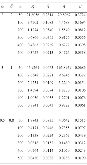
generated and then computed the MLEs and LSEs of a and b with 10000 repetitions. We then compared the performance of these estimates in terms of their biases and mean square errors (MSE). We reported the biases and MSEs of these estimates in Tables 1-2, for different values of n and (a b . , ) From Tables 1-2, it is observed that both estimates are biased but asymptotically unbiased. Also, as the sample size n increases, the bias and MSEs of the estimators decreases as expected.
Table 1: Bias of MLEs and LSEs for some parameter values of a and b
a b n aˆ ˆ a b 2 2 50 1.3612 0.0939 1.5310 0.1023 100 0.5514 0.0420 0.5679 0.0413 200 0.2525 0.0196 0.2718 0.0226 300 0.1734 0.0146 0.1764 0.0151 400 0.1341 0.0120 0.1395 0.0137 500 0.1031 0.0094 0.1053 0.0102 3 1 50 2.1219 0.0398 2.4204 0.0439 100 0.8103 0.0178 0.8230 0.0196 200 0.3690 0.0085 0.3904 0.0107 300 0.2532 0.0063 0.2573 0.0071 400 0.1809 0.0044 0.1837 0.0050 500 0.1532 0.0043 0.1553 0.0051 0.5 0.8 50 0.4662 0.0908 0.6711 0.1070 100 0.1950 0.0402 0.2800 0.0435 200 0.0912 0.0173 0.1241 0.0131 300 0.0620 0.0109 0.0849 0.0073 400 0.0477 0.0088 0.0648 0.0059 500 0.0392 0.0071 0.0506 0.0039
Table 2: MSEs of MLEs and LSEs for some parameter values of a and b a b n aˆ bˆ a b 2 2 50 21.6056 0.2314 29.8067 0.3724 100 3.4502 0.1083 4.4688 0.1694 200 1.1274 0.0540 1.5549 0.0812 300 0.6866 0.0365 0.9176 0.0556 400 0.4863 0.0269 0.6272 0.0398 500 0.3657 0.0213 0.4724 0.0318 3 1 50 46.9261 0.0463 165.8959 0.0686 100 7.6548 0.0221 9.6245 0.0322 200 2.4231 0.0109 3.2240 0.0154 300 1.4694 0.0074 1.8830 0.0106 400 1.0050 0.0055 1.2791 0.0076 500 0.7841 0.0043 0.9722 0.0061 0.5 0.8 50 1.9843 0.0835 4.0642 0.1515 100 0.4171 0.0446 0.7355 0.0797 200 0.1338 0.0224 0.2367 0.0439 300 0.0818 0.0152 0.1480 0.0312 400 0.0564 0.0114 0.1050 0.0243 500 0.0430 0.0088 0.0788 0.0190
5. REAL DATA ANALYSIS
In this section, we illustrate the ability of the APTP distribution. We fit this distribution to two real data sets and compare the results with the distributions in the literature. In order to compare the models, we used following three criterions: Akaike Information Criterion(AIC), Bayesian Information Criterion (BIC) and log-likelihood ( ) values, where the lower values of AIC, BIC and the upper value of values for models indicate that these models could be chosen as the best model to fit the data sets.
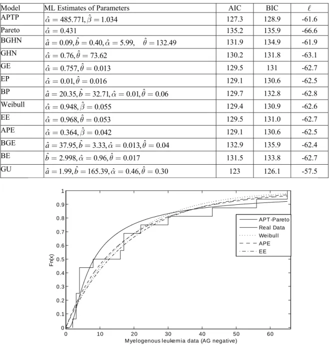
First real data: First real data set is given in Feigl and Zelen [10] for the patients who died of acute myelogenous leukemia. Feigl and Zelen [10] represent observed survival times (weeks) for AG negative. The data set is: 56, 65, 17, 17, 16, 22, 3, 4, 2, 3, 8, 4, 3, 30, 4, 43. APTP, Weibull, Alpha-Power Exponential( Mahdavi and Kundu [8]), Exponentiated Exponential (Gupta and Kundu, [3]), Beta Generalized-Exponential (BGE) (Barreto-Souza et al. [11]), Beta-Exponential (BE) (Nadarajah and Kotz [12]), Beta-Pareto (BP)(Akinsete et al. [13]), Generalized Exponential (GE)(Gupta and Kundu [14]), Exponential Poisson (EP) (Kus [15]), Beta Generalized Half-Normal (BGHN) (Pescim et al. [16]), Generalized Half-Normal (GHN)(Cooray and Ananda [17]) and Gamma-Uniform (GU) (Torabi
and Montazeri [18]) distributions are fitted to data. Table 3 shows that the APTP distribution gives a better fit than the other models for all criteria except GU distribution.
Table 3. Results of AIC, BIC and log-likelihood for APTP and other distributions for the data set
Model ML Estimates of Parameters AIC BIC
APTP aˆ =485.771,bˆ =1.034 127.3 128.9 -61.6 Pareto a =ˆ 0.431 135.2 135.9 -66.6 BGHN aˆ=0.09,bˆ=0.40,aˆ =5.99, ˆq =132.49 131.9 134.9 -61.9 GHN aˆ =0.76,qˆ=73.62 130.2 131.8 -63.1 GE aˆ =0.757,qˆ=0.013 129.5 131 -62.7 EP aˆ =0.01,qˆ=0.016 129.1 130.6 -62.5 BP aˆ=20.35,bˆ=32.71,aˆ=0.01,qˆ=0.06 129.7 132.8 -62.8 Weibull aˆ =0.948,bˆ =0.055 129.4 130.9 -62.6 EE aˆ =0.968,qˆ=0.053 129.5 131.0 -62.7 APE aˆ =0.364,bˆ=0.042 129.1 130.6 -62.5 BGE aˆ=37.95,bˆ=3.33,aˆ =0.013,qˆ=0.04 132.9 135.9 -62.4 BE bˆ=2.998,aˆ =0.96,qˆ=0.017 131.5 133.8 -62.7 GU aˆ=1.99,bˆ=165.39,aˆ =0.46,qˆ=0.30 123 126.1 -57.5
Figure 3. Empirical and some fitted distribution functions based on myelogenous leukemia data
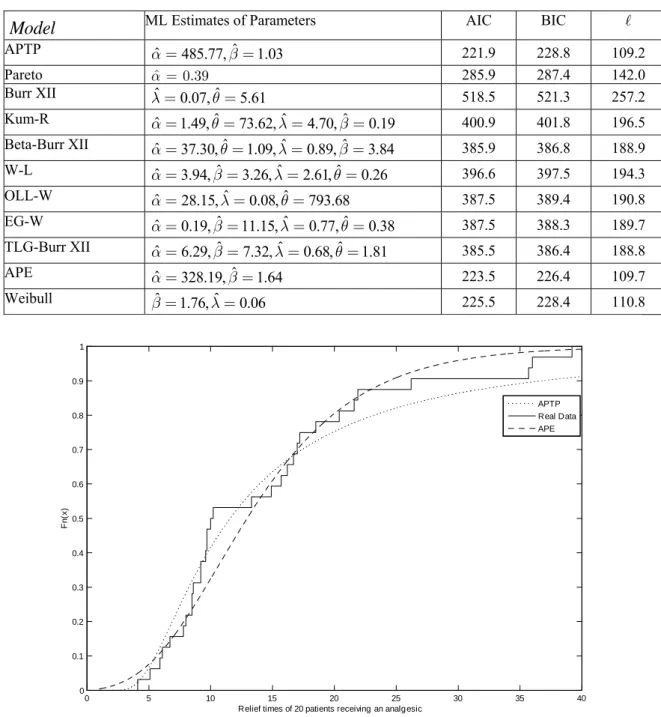
Second real data set: The real dataset is taken from Nassar and Nada [19], which gives the relief times of 32 patients receiving an analgesic. The data are: 5.9, 20.4, 14.9, 16.2, 17.2, 7.8, 6.1, 9.2, 10.2, 9.6, 13.3, 8.5, 21.6, 18.5, 5.1,6.7, 17, 8.6, 9.7, 39.2, 35.7, 15.7, 9.7, 10, 4.1, 36, 8.5, 8, 9.2, 26.2, 21.9,16.7, 21.3, 35.4, 14.3, 8.5, 10.6, 19.1, 20.5, 7.1, 7.7, 18.1, 16.5, 11.9, 7, 8.6,12.5, 10.3, 11.2, 6.1, 8.4, 11, 11.6, 11.9, 5.2, 6.8, 8.9, 7.1, 10.8. APTP, Burr XII distribution by Burr[20], Kumaraswamy Rayleigh (Kum-R) by Rashwan [21], Beta Bur XII (Beta-BXII) by Paranaíba et al.[22], Weibull Lomax (W-L) by Tahir et al. [23]. Odd log-logistcWeibull (OLL-W) by Cruz et al. [24], and Exponentiated Generated Weibull (EG-W) by Cordeiro et al. [25] distributions are fitted to data. From Table 4, it is clear that the APTP distribution provides the overall best fit and therefore could be chosen as the most adequate model among the fitted models to second data.
0 10 20 30 40 50 60 0 0.1 0.2 0.3 0.4 0.5 0.6 0.7 0.8 0.9 1
Myelogenous l eukemia data (AG negative)
F n (x ) APT -Pareto Real Data Weibul l APE EE
Table 4. Results of AIC and log-likelihood for APTP and other distributions for the data set.
Model
ML Estimates of Parameters AIC BIC APTP aˆ =485.77,bˆ=1.03 221.9 228.8 109.2 Pareto a =ˆ 0.39 285.9 287.4 142.0 Burr XII ˆl=0.07,qˆ=5.61 518.5 521.3 257.2 Kum-R aˆ=1.49,qˆ=73.62,lˆ=4.70,bˆ=0.19 400.9 401.8 196.5 Beta-Burr XII aˆ=37.30,qˆ=1.09,lˆ=0.89,bˆ=3.84 385.9 386.8 188.9 W-L aˆ=3.94,bˆ=3.26,lˆ=2.61,qˆ=0.26 396.6 397.5 194.3 OLL-W aˆ=28.15,lˆ=0.08,qˆ=793.68 387.5 389.4 190.8 EG-W aˆ=0.19,bˆ=11.15,lˆ=0.77,qˆ=0.38 387.5 388.3 189.7 TLG-Burr XII aˆ =6.29,bˆ=7.32,lˆ=0.68,qˆ=1.81 385.5 386.4 188.8 APE aˆ =328.19,bˆ=1.64 223.5 226.4 109.7 Weibull ˆb=1.76,lˆ=0.06 225.5 228.4 110.8
Figure 4. Empirical and some fitted distribution functions based on relief times data
6. CONCLUSION
In this study, APT family is considered with baseline Pareto distribution. ML and LS estimation are discussed for the parameters. An application of the APTP distribution to a real data set is given to demonstrate that this distribution can be used quite effectively to provide better fit than other available models.
REFERENCES
[1] Azzalini A., A class of distributions which includes the normal ones, Scandinavian journal of statistics, 24 (1985), 171-178. 0 5 10 15 20 25 30 35 40 0 0.1 0.2 0.3 0.4 0.5 0.6 0.7 0.8 0.9 1
Relief times of 20 patients receiving an analg esic
F n (x ) APTP Real Data APE
[2] Mudholkar G.S. and Srivastava D.K., Exponentiated weibull family for analyzing bathtub failure-rate data, IEEE Transactions on Reliability, 42-2 (1993), 299-302.
[3] Gupta R.C., Gupta P.L. and Gupta R.D., Modeling failure time data by lehman alternatives, Communications in Statistics-Theory and Methods, 27-4 (1998), 887-904.
[4] Gupta R.D. and Kundu D., Exponentiated exponential family: an alternative to gamma and Weibull distributions, Biometrical Journal: Journal of Mathematical Methods in Biosciences, 43-1 (2001), 117-130.
[5] Marshall A.W. and Olkin I., A new method for adding a parameter to a family of distributions with application to the exponential and weibull families, Biometrika, 84-3 (1997), 641-652.
[6] Eugene N., Lee C. and Famoye F., Beta-normal distribution and its applications, Communications in Statistics-Theory and Methods, 31-4 (2002), 497-512.
[7] Alzaatreh A., Lee C. and Famoye F., A new method for generating families of continuous distributions, Metron, 71-1 (2013), 63-79.
[8] Mahdavi A. and Kundu D., A new method for generating distributions with an application to exponential distribution, Communications in Statistics - Theory and Methods, 46-13 (2017), 6543-6557.
[9] Lagarias J.C., Reeds J.A., Wright M.H. and Wright P.E., Convergence Properties of the Nelder-Mead Simplex Method in Low Dimensions, SIAM Journal of Optimization, 9-1 (1998), 112-147. [10] Feigl P. and Zelen M., Estimation of Exponential Survival Probabilities with Concomitant
Information, Biometrics, 21-4 (1964), 826-838.
[11] Barreto-Souza W., Santos A.H.S. and Cordeiro G.M., The Beta generalized exponential distribution, Statist. Comput. Simul., 80 (2010), 159-172.
[12] Nadarajah S. and Kotz S., The Beta exponential distribution, Reliability Engrg. System Safety, 91 (2006), 689-697.
[13] Akinsete A., Famoye F. and Lee C. The Beta-Pareto distribution, Statistics, 42-6(2008), 547-563. [14] Gupta R.D. and Kundu D., Generalized exponential distributions, Australian and New Zealand
Journal of Statistics, 41-2 (1999), 173-188.
[15] Kus C, A new lifetime distribution, Comput. Statist. Data Anal., 51(2007), 4497-4509.
[16] Pescim R.R., Dem´etrio C.G.B., Cordeiro G.M., Ortega E.M.M. and Urbano M.R., The Beta generalized half-Normal distribution, Comput. Statist. Data Anal., 54 (2009), 945-957.
[17] Cooray K. and Ananda M.M.A., A generalization of the half-normal distribution wit applications to lifetime data, Comm. Statist. Theory Methods, 37 (2008), 1323-1337.
[18] Torabi H. and Montazeri N.H., The Gamma-Uniform distribution ans its applications, Kybernetika, 48-1 (2012), 16-30.
[19] Nassar M.M. abd Nada N.K., The beta generalized Pareto distribution, Journal of Statistics: Advances in Theory and Applications, 6 (2011), 1-17.
[20] Burr, I.W., Cumulative frequency functions, Annals of Mathematical Statistics, 13(1942), 215-232. [21] Rashwan N.I., A note on Kumaraswamy exponentiated Rayleigh distributioni, Journal of Statistical
Theory and Applications, 5 (2016), 286-295.
[22] Paranaíba P.F., Ortega E. M., Cordeiro G. M. and Pescim R.R., The beta Burr XII distribution with application to lifetime data, Computational Statistics and Data Analysis, 55-2 (2011), 1118-1136. [23] Tahir, M.H., Cordeiro G. M., Mansoor M. and Zubair M., The Weibull-Lomax distribution:
properties and applications, Hacettepe Journal of Mathematics and Statistics, 44-2 (2015), 461-480. [24] Cruz J.N.D., Ortega E.M. and Cordeiro G.M., The log-odd log-logistic Weibull regression model: modelling, estimation, influence diagnostics and residual analysis, Journal of Statistical Computation and Simulation, 86-8 (2016), 1516-1538.
[25] Cordeiro G.M., Gomes A.E., da-Silva C.Q. and Ortega E.M., The beta exponentiated Weibull distribution, Journal of Statistical Computation and Simulation, 83-1 (2013), 114-138.