Başlık: Drought analysis of the Seyhan Basin by using standardized precipitation ındex (spı) and l-momentsYazar(lar):TOPÇU, Emre; SEÇKİN, Neslihan Cilt: 22 Sayı: 2 Sayfa: 196-215 DOI: 10.1501/Tarimbil_0000001381 Yayın Tarihi: 2016 PDF

(1)

Tarım Bilimleri Dergisi

Tar. Bil. Der.

Dergi web sayfası: www.agri.ankara.edu.tr/dergi

Journal of Agricultural Sciences

Journal homepage:

www.agri.ankara.edu.tr/journal

TARIM BİLİMLERİ DERGİSİ

—

JOURNAL OF AGRICUL

TURAL SCIENCES

22 (2016) 196-215

Drought Analysis of the Seyhan Basin by Using Standardized

Precipitation Index (SPI) and L-moments

Emre TOPÇUa_{, Neslihan SEÇKİN}a

a_{Çukurova University, Faculty of Engineering and Architecture, Department of Civil Engineering, 01330, Adana, TURKEY} ARTICLE INFO

Research Article

Corresponding Author: Neslihan SEÇKİN, E-mail: nseckin@cu.edu.tr, Tel: +90 (322) 338 60 84 Received: 03 April 2014, Received in Revised Form: 21 January 2015, Accepted: 28 January 2015

ABSTRACT

The aim of this study is to monitor drought in the Seyhan Basin by using Standardized Precipitation Index (SPI) based on a long term monthly precipitation of 11 meteorological stations and secondly, to also carry out regional frequency analysis using the index flood procedure coupled with the L-moments method based on recorded precipitation data of the most drought month for each year acquired from Standardized Precipitation Index method for each station. The SPI values of each station for 3, 6, 9 and 12-month time scales were calculated. According to the results, all stations are on the boundary of drought. Research results show that the wettest station is Ulukışla and the most drought station is Karaisalı with respect to the average SPI values. According to the drought frequency values, however, the station having the highest drought occurrence frequency is the Karaisalı station, whereas the station having the lowest drought frequency is the Tufanbeyli station. Results show that the Seyhan Basin is on the boundary of drought and mildly wet. Drought occurrence frequency is 47.7%. L-moments method was used to define homogenous regions. Homogenous regions for 3 and 6-month time scales minimum precipitation series couldn’t be obtained while homogenous regions for 9-month time scale minimum precipitation series were obtained only by dividing the whole basin into two parts. The whole basin is homogenous for the 12-month time scale minimum precipitation series. The Pearson Type 3 distribution is found to be most suitable for two homogenous sub-basins regarding 9-month time scale minimum precipitation series, whereas the Generalized Normal distribution is found to be most suitable for the whole basin with respect to 12-month time scale minimum precipitation series.

Keywords: The Seyhan Basin; Standardized precipitation index (SPI); L-moments; Climate change; Rainfall

L-momentler ve Standart Yağış İndeksi (SYİ) Yardımıyla Seyhan

Havzası Kuraklık Analizi

ESER BİLGİSİ Araştırma Makalesi

Sorumlu Yazar: Neslihan SEÇKİN, E-posta: nseckin@cu.edu.tr, Tel: +90 (322) 338 60 84 Geliş Tarihi: 03 Nisan 2014, Düzeltmelerin Gelişi: 21 Ocak 2015, Kabul: 28 Ocak 2015

ÖZET

Bu çalışmanın amacı Seyhan Havzası’ndaki 11 meteorolojik istasyonun uzun dönem aylık yağış değerlerine dayalı Standart Yağış İndeksi’ni (SYİ) kullanarak kuraklık takibi yapmak ve ayrıca ikinci olarak her istasyonun her yılı için

(2)

Drought Analysis of the Seyhan Basin by Using Standardized Precipitation Index (SPI) and L-moments, Topçu & Seçkin

197

Ta r ı m B i l i m l e r i D e r g i s i – J o u r n a l o f A g r i c u l t u r a l S c i e n c e s 22 (2016) 196-215

1. Introduction

Drought is defined elementarily as the deficiency of the customary total precipitations and dry air for the water basins, in any piece of land of the world for a specific timeframe by both hydrologist and those concerned. Drought is one of the hardest, imponderable and unstoppable climatic incidents like floods, hurricanes etc. There are in general three types of droughts taken into account, they are, meteorological, agricultural and hydrological drought (Wilhite & Glantz 1987). Meteorological drought is wholly relevant to weather conditions; it is described as decrease in the normal amount of precipitations relative to at least recorded 30 years of precipitation series. Meteorological drought influences the other two types of drought and begins before them. Agricultural drought is considered as the lack of soil moisture which leads to wilting and plant death in farmlands, even if there are adequate precipitations and water resources, agricultural drought could occur because of the excessive usage of water and may be unnecessary agricultural activities. If moisture free wind blows, the intensity of the drought will be exacerbated. Hydrological drought occurs when the precipitation and amount of water in reservoirs are enough but either population to make use of the water is high or rural activities and irrigation activities are excessive. So when hydrological drought happens, urban life definitely comes across problems and hydroelectric power production and sprinkler systems will be affected

adversely. No wonder, this engenders economic crisis and decrease financial support. In a long period of dry weather, we observed a drought of more than 2 weeks diminished the soil moisture quite slowly and if it lasts longer, it raises maximum evaporation rate then all water reservoirs even subsurface water may clear away. For this reason hydrologists name the drought as creeping phenomenon.

The amount of precipitation shortage impinges upon nearly all aspects of the social, environmental and economic life of a society. In terms of social life, drought has gross impacts such as; augmentation of poverty, migration, politic clashes, decrease in life, physical and mental stress for human body. In terms of environmental life, shortage of drinking water and food, rising plant, animal and human diseases, increase in desertification and wind erosion rate, extinction of animal and rare plant species. In terms of economic life, decrease in tourism, commercial livestock raising, hydroelectric power and energy, increase in food prices. At present, scientists have discovered that drought and other climatic incidents are caused by not only prominent and notorious global warming but also sun spots and sun flares, scientists are pondering that sun spots and sun flares will be increased at highest level in 2000s, so this will raise the radiation level and global heat (Vardiman 2008). The change in the amount of radiation and heat means that atmospheric pressure will be influenced unfavorably and climatic fatal affairs which already cannot be determined properly Standart Yağış İndeksi yönteminden elde edilen en kurak ayının yağış değerlerine indeks taşkın yöntemine dayalı L-momentler metodu uygulanarak bölgesel frekans analizi yapmaktır. Her istasyonun 3, 6, 9 ve 12 ay süreli SYİ değerleri hesaplanmıştır. Sonuçlara göre bütün istasyonlar kuraklık sınırındadır. Ortalama SYİ değerlerine göre en ıslak istasyon Ulukışla iken en kurak istasyon Karaisalı’dır. Kuraklık frekans değerlerine göre ise kuraklık meydana gelme frekansı en yüksek Karaisalı istasyonu iken kuraklık meydana gelme frekansı en düşük istasyon Tufanbeyli’dir. Sonuçlar gösteriyor ki, Seyhan havzası kuraklık sınırında ve biraz ıslaktır. Kuraklık oluşma frekansı % 47.7’dir. L-momentler metodu homojen bölgeleri belirlemek için kullanılmıştır. 3 ve 6 aylık minimum yağış serilerinden homojen bölgeler elde edilemezken 9 aylık minimum yağış serisinde havza iki kısma ayrılarak homojen alt havzalar elde edilmiştir. 12 aylık minimum yağış serisinde ise tüm havza homojen çıkmıştır. 9 aylık minimum yağış serisi için homojen iki alt havzaya en iyi uyan dağılım Pearson Tip 3 dağılımı iken 12 aylık minimum yağış serisi için tüm havzaya uyan en iyi dağılım Genelleştirilmiş Normal dağılım olmuştur.

Anahtar Kelimeler: Seyhan Havzası; Standart yağış indeksi (SYİ); L-momentler; İklim değişikliği; Yağış

(3)

L-momentler ve Standart Yağış İndeksi (SYİ) Yardımıyla Seyhan Havzası Kuraklık Analizi, Topçu & Seçkin

198

Ta r ı m B i l i m l e r i D e r g i s i – J o u r n a l o f A g r i c u l t u r a l S c i e n c e s 22 (2016) 196-215 and occur unpredictably mostly come out. There are

some studies about impacts of large scale volcanic eruptions and air pollution on occurring droughts. The other exotic factors have force on droughts are aerosol gases sprayed from colossal volcanic eruptions and industrial exhaust gases. This gases such as CO2 (carbon dioxide) and SO2 (sulfur

dioxide) alter the patterns of precipitations and have greenhouse effect which constitute the global warming. Heat and radiation coming from the sun could not be reflected to the space because of the greenhouse effect (NASA 2010a).

The beginning pattern of precipitation commences with the collision of little microscopic rain drops, they collide or bond, but the air is polluted and covered by greenhouse effected gases, then the rain drops could not become together and consist of precipitation, this gives rise to drought (Fang et al 2013). A good example of this is the Pinatubo volcano, which erupted in 1991 and is one of the largest volcanic eruption in the 20th century, as there was decrease in the amount of precipitation for some seasons, sprayed gases moved with strong winds around the World (Trenberth & Dai 2007). As known, northern hemisphere’s heat increases rapidly rather than southern hemisphere, since there are larger continents in the northern hemisphere than the southern hemisphere. In the south, oceans cover larger places than the mainlands. The mainland cools down and heats up more quickly than water covered areas. During the period 1997-2006 average temperature of the northern hemisphere had increased almost 0.53 °C (0.27 °C for the southern hemisphere) in comparison with the period 1961-1990 (WMO 2007). Separately, sea ice volume affects the climate and then droughts.

Not so far or above the “Planet Earth”, there is one more unfavorable driver which is called ‘heat island’. Wide concrete roads, dark structures are deprived of green areas in metropolitan cities induced heat island. Since energy and heat coming from the sun in daytime absorbed by this type of factors mentioned. So, the difference in temperatures between metropolitan cities and very near rural areas can be 10 °C or more, this of course affects the rain pattern (NASA 2010b).

Drought has short or long periods; it depends on the characteristics of the drought. In the world, principally middle zones of the broad continents such as America, Asia and Africa have the wildest drought events by reason of being far from warm sea and sea moisture. The most unpredictable points of drought are the beginning and ending time. Intensity of forthcoming drought can never be measured but only predicted from extreme dry periods which happened before, scientist and hydrologist are interested particularly on this point. Nowadays technology may not detect characteristics of droughts and other intense climatic events flawlessly, especially when to start and end, but by utilizing various mathematic algorithms these problems could be clarified. Knowledge of the characteristics of the drought is vital for water running and urban organizations. There have been a lot of drought monitoring tools developed by hydrologists in literature such as Palmer Drought Severity Index (PDSI), Erinc and De Martonne methods. In this paper Standardized Precipitation Index (SPI) drought monitoring tool developed by (McKee et al 1993) is used. It is significant to scrutinize the data for the frequency of occurrence of drought, extreme precipitations cause floods, whereas minimum precipitations cause droughts. Frequency analysis method is used prevalently to estimate the droughts and floods, precipitation time series are a must for planning hydraulic structures, and researchers usually use the maximum precipitation data to estimate flash floods. However, in this paper, minimum precipitation depths instead of maximum precipitation depths were employed to monitor the drought. For frequency analysis, L-moments method developed by (Hosking 1986; 1990) was used by utilizing precipitation data of the most drought months which are detected from SPI results of each year for all stations.

2. Material and Methods

2.1. Material

In this study, the Seyhan Basin, one of the biggest and fertile basins in Turkey, North Mediterranean and Europe, is selected as a study area and comes after the Nile Basin in terms of size. The Seyhan Basin is one of the 26 basins in Turkey and located in the south.

(4)

199

Ta r ı m B i l i m l e r i D e r g i s i – J o u r n a l o f A g r i c u l t u r a l S c i e n c e s 22 (2016) 196-215 The Seyhan Basin’s area is 20450 km2_{and constitutes}

of the 2.82% of Turkey. The Seyhan Basin provides both economic and agricultural resources to Turkey and the world. This basin has innumerable biological species. Therefore researchers focus on Seyhan Basin for drought or other issues. For instance, Gurkan (2005) simulated for both based on decrease in precipitation amount and increase in temperature and potential evapotranspiration. Fujihara et al (2008) used the inverse approach to model hydrological risk and vulnerability to changing climate conditions in the Seyhan River basin. Sen et al (2008) aimed a research to predict future climate and its possible impact on water resources and agricultural water use in Seyhan basin for the period 2071-2100 by using climate model RegCM3, Topcu (2013) carried out a thesis to assess the drought in Seyhan Basin and analyzed monthly precipitation for SPI and used outputs for L-moments. Selek & Tuncok (2014) conducted a study to determine the basis for climate change adaptation of water resources management policies in Seyhan River basin. It was determined that even though there was no water stress in Seyhan basin in 2010, many parts of the basin were expected to suffer significant shortages over the coming years. Altın & Barak (2012) calculated the Erinc Drought Index by using precipitation series of 29 meteorological stations for the period of 1970-2009 in Seyhan Basin. Climate type is determined and mapped.

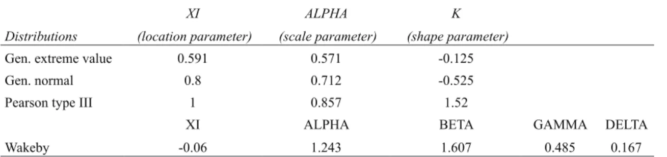
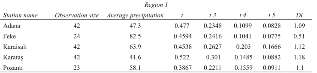
In this study at least recorded 20 years of precipitation time series are used for analysis. Totally 11 meteorological stations are employed for this dissertation, the main characteristics of the stations are shown in Table 1. Data of the stations are obtained from Turkish State Meteorological Service. Locations of stations are shown in Figure 1. Precipitation depths increase from the north to the south unlike temperature due to high geographic formations.

Figure 1- Locations of the stations in the Seyhan Basin Şekil 1- İstasyonların Seyhan Havzası’ndaki konumları Table 1- Main characteristics of stations

Çizelge 1- İstasyonların temel karakteristikleri

Station name Number Observation years Elevation (m) Latitude Longitude Size (year)

Adana 17351 1970-2012 27 37° 00’ 30” N 35° 20’ 67” E 43 Çamardı 6893 1970-1994 1500 37° 49’ 54” N 34° 59’ 03” E 25 Feke 6902 1970-1994 620 37° 49’ 04” N 35° 54’ 46” E 25 Karaisalı 17936 1970-2012 241 37° 15’ 05” N 35° 03’ 47” E 43 Karataş 17981 1970-2012 22 36° 33’ 51” N 35° 22’ 96” E 43 Pınarbaşı 17802 1970-2010 1500 38° 43’ 17” N 36° 23’ 39” E 41 Pozantı 17934 1970-1993 750 37° 25’ 00” N 34° 53’ 00” E 24 Sarız 17840 1970-2011 1500 38° 28’ 47” N 36° 29’ 49” E 42 Tomarza 17837 1970-2010 1400 38° 26’ 00” N 35° 48’ 00” E 41 Tufanbeyli 6204 1986-2012 1350 38° 15’ 54” N 36° 13’ 13” E 27 Ulukışla 17906 1970-2012 1453 37° 33’ 00” N 34° 29’ 00” E 43

(5)

200

Ta r ı m B i l i m l e r i D e r g i s i – J o u r n a l o f A g r i c u l t u r a l S c i e n c e s 22 (2016) 196-215

2.2. Method

2.2.1. Standardized precipitation index (SPI) method

Droughts and floods are widespread subject of the hydraulic engineers and researchers. This method is used commonly to monitor the drought because of the simple algorithm and rapid response. The SPI was developed by (McKee et al 1993) for providing drought information in Colorado. Seasonal (3, 6-month time scale) or long period (9, 12, 24, 48-month time scale) drought can be analyzed, which affects all types of water resources even subsurface water. Soil moisture is affected immediately from abrupt precipitation changes. Hence, 3 or 6-month time scale monitoring is preferred. On the other hand, underground water, rivers and reservoirs do not respond rapidly to swift precipitation changes. Therefore, 12-month or long period time scale (24, 48, 72-month) monitoring is chosen. There are lots of studies about Standardized Precipitation Index for monitoring drought all around the world like (McKee et al 1993; Edwards & McKee 1997; Guttman 1999; Türkes 1999; Kömüscü 2001; Lloyd-Hughes & Saunders 2002; Tonkaz 2006; Li et al 2008; Abolverdi & Khalili 2010; Keskin & Sorman 2010). Anlı (2014) carried out a study to analysis meteorological drought in provinces of South Eastern Anatolia Region by using temporal variation of reference evapotranspiration (ET₀) and RDI (Reconnaissance Drought Index). Study results show that significant increasing trends for reference evapotranspiration have been detected and according to RDI, mild drought has been experienced in general. In addition, there have been a significant amount of events where moderate and severely droughts occurred. Guenang & Kamga (2014) computed SPI using 55 years of precipitation data recorded 24 observation stations in Cameroon. Four statistical distribution functions (gamma, exponential, Weibull and lognormal) are fitted to data. Drought thresholds determined. McRoberts & Nielsen-Gammon (2012) developed high-resolution drought-monitoring tool to assess drought on multiple time scales using the SPI. Regional frequency

analysis is performed. Dutra et al (2013) assessed the predictive capabilities of an integrated drought monitoring and seasonal forecasting system (up to 5 months lead time) based on SPI. The forecasts were evaluated over four basins in Africa. Jha et al (2013) computed the SPI with monthly precipitation dataset for each of the 14 mainland agro climatic zones of India. Showed that only six out of 14 mainlands have a significant trend during summer monsoon. Blain (2012) carried out analyses by evaluating the normality assumption of the SPI distributions. Observed that Pearson III distribution was better than the Gamma 2-parameter distribution. Xie et al (2013) investigated the spatiotemporal variability of drought incidence in Pakistan during 1960-2007 by SPI for 3, 6 and 12-month scales. Analysis revealed that droughts are wide-spread and often occur over large areas. Simsek & Cakmak (2010) analyzed the drought experience in 2007-2008 Agricultural Year of Turkey. The drought was evaluated by using SPI, Percent of Normal Index (PNI) and the analyses of precipitation and temperature analysis. The SPI is the non-dimensional drought index. This index is computed for long time precipitation series for the preferred time scales. The SPI calculated by Equation 1.

5

Study results show that significant increasing trends for reference evapotranspiration have been detected and according to RDI, mild drought has been experienced in general. In addition, there have been a significant amount of events where moderate and severely droughts occurred. Guenang & Kamga (2014) computed SPI using 55 years of precipitation data recorded 24 observation stations in Cameroon. Four statistical distribution functions (gamma, exponential, Weibull and lognormal) are fitted to data. Drought thresholds determined. McRoberts & Nielsen-Gammon (2012) developed high-resolution drought-monitoring tool to assess drought on multiple time scales using the SPI. Regional frequency analysis is performed. Dutra et al (2013) assessed the predictive capabilities of an integrated drought monitoring and seasonal forecasting system (up to 5 months lead time) based on SPI. The forecasts were evaluated over four basins in Africa. Jha et al (2013) computed the SPI with monthly precipitation dataset for each of the 14 mainland agro climatic zones of India. Showed that only six out of 14 mainlands have a significant trend during summer monsoon. Blain (2012) carried out analyses by evaluating the normality assumption of the SPI distributions. Observed that Pearson III distribution was better than the Gamma 2-parameter distribution. Xie et al (2013) investigated the spatiotemporal variability of drought incidence in Pakistan during 1960-2007 by SPI for 3, 6 and 12-month scales. Analysis revealed that droughts are wide-spread and often occur over large areas. Simsek & Cakmak (2010) analyzed the drought experience in 2007-2008 Agricultural Year of Turkey. The drought was evaluated by using SPI, Percent of Normal Index (PNI) and the analyses of precipitation and temperature analysis. The SPI is the non-dimensional drought index. This index is computed for long time precipitation series for the preferred time scales. The SPI calculated by Equation 1.

SPI = (Xİ− X̅)/ σ (1)

Where; SPI, standardized precipitation index;

X

İ, data point;

X̅

, mean;

𝜎𝜎

, standard deviation of the data

The gamma distribution is convenient for precipitation series and the distribution parameters can be calculated by maximum likelihood approximation of Thom (1958). If precipitation data has zero values, mixed distribution by Thom (1951) can be used for incorporation of zero probability and non-zero probabilities (Equation 2).

H(x) = q + (1-q) G(x) (2)

Where; q, the probability of zero precipitation; G(x), the gamma cumulative probability function. Probabilities calculated by Equation 2 are transformed into the standard normal distribution for calculation of the SPI values (Guttman 1998).

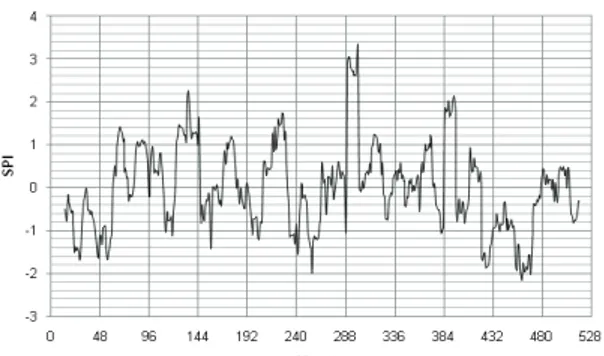
SPI method shows the drought category corresponds to output values (Table 2). If the SPI gives negative values, it means there is drought and lack of precipitation; if the SPI gives positive values, it means there is no drought and enough precipitation. Yet, the negative values are getting lower, the degree of the drought shifts from no drought to extremely drought and then catastrophe bursts. And same for the positive values, if the positive values are getting higher the degree of the drought shifts from no drought to extremely wet and flash floods are seen. The drought frequency of a station is obtained by dividing drought event size by total observation size. Frequency values show us how often drought conditions happen in a station for a prespecified time scale.

(1) Where; SPI, standardized precipitation index;

5

SPI = (Xİ− X̅)/ σ (1)

X

İ, data point;

X̅

, mean;

𝜎𝜎

H(x) = q + (1-q) G(x) (2)

, data point;

5

SPI = (Xİ− X̅)/ σ (1)

X

İ, data point;

X̅

, mean;

𝜎𝜎

H(x) = q + (1-q) G(x) (2)

, mean;

5

SPI = (Xİ− X̅)/ σ (1)

X

İ, data point;

X̅

, mean;

𝜎𝜎

H(x) = q + (1-q) G(x) (2)

5

SPI = (Xİ− X̅)/ σ (1)

_X

_İ, data point;

_X̅

, mean;

_𝜎𝜎

, standard deviation of the data The gamma distribution is convenient for precipitation series and the distribution parameters can be calculated by maximum likelihood approximation of Thom (1958). If precipitation data has zero values, mixed distribution by Thom (1951) can be used for incorporation of zero probability and non-zero probabilities (Equation 2).

H(x) = q + (1-q) G(x) (2)

(2) Where; q, the probability of zero precipitation; G(x), the gamma cumulative probability function. Probabilities calculated by Equation 2 are transformed into the standard normal distribution for calculation of the SPI values (Guttman 1998).

(6)

201

Ta r ı m B i l i m l e r i D e r g i s i – J o u r n a l o f A g r i c u l t u r a l S c i e n c e s 22 (2016) 196-215 SPI method shows the drought category

corresponds to output values (Table 2). If the SPI gives negative values, it means there is drought and lack of precipitation; if the SPI gives positive values, it means there is no drought and enough precipitation. Yet, the negative values are getting lower, the degree of the drought shifts from no drought to extremely drought and then catastrophe bursts. And same for the positive values, if the positive values are getting higher the degree of the drought shifts from no drought to extremely wet and flash floods are seen. The drought frequency of a station is obtained by dividing drought event size by total observation size. Frequency values show us how often drought conditions happen in a station for a prespecified time scale.

Table 2- Standardized precipitation index categories Çizelge 2- Standart yağış indeksi kategorileri

SPI index values Drought category

2.00 or more Extreme Wet

1.50 - 1.99 Severe Wet 1.00 - 1.49 Moderate Wet 0.0 - 0.99 Mild Wet 0.0 - (-0.99) Mild Drought (-1.00) - (-1.49) Moderate Drought (-1.50) - (-1.99) Severe Drought

(-2.00) or less Extreme Drought

2.2.2. Index-flood method

Index flood method is a reliable procedure as to pooling summary statistics from different data samples. Its early applications were based on flood data in hydrology (Dalrymple 1960). However, Hosking & Wallis (1997) pointed out that this method can be applicable to every kind of data.

According to the index-flood method, the exceedance probability distribution of annual peak discharge is accepted as identical for hydrologically homogeneous regions except for a site-specific scaling factor called the index flood (Dalrymple 1960; Hosking & Wallis 1997).

The important physiographic and meteorological characteristics of a basin are reflected by this index flood parameter. In this method, the relationship in Equation 3 is recommended to estimate the flood quantile Q_T.

6

Table 2- Standardized precipitation index categories Çizelge 2- Standart yağış indeksi kategorileri

SPI index values Drought category

2.00 or more Extreme Wet

1.50 - 1.99 Severe Wet 1.00 - 1.49 Moderate Wet 0.0 - 0.99 Mild Wet 0.0 - (-0.99) Mild Drought (-1.00) - (-1.49) Moderate Drought (-1.50) - (-1.99) Severe Drought

(-2.00) or less Extreme Drought

2.2.2. Index-flood method

Index flood method is a reliable procedure as to pooling summary statistics from different data samples. Its early applications were based on flood data in hydrology (Dalrymple 1960). However, Hosking & Wallis (1997) pointed out that this method can be applicable to every kind of data.

According to the index-flood method, the exceedance probability distribution of annual peak discharge is accepted as identical for hydrologically homogeneous regions except for a site-specific scaling factor called the index flood (Dalrymple 1960; Hosking & Wallis 1997).

The important physiographic and meteorological characteristics of a basin are reflected by this index flood parameter. In this method, the relationship in Equation 3 is recommended to estimate the flood quantile QT.

Q

T

= q

T

μ

i (3)

Where; T, return period at site i; μ, the product of index flood (average likely flood); q, the regional growth factor. μ is also the function basin area and slope. q is a dimensionless frequency distribution quantity common to all sites within a hydrologic homogeneous region.

A relationship based on available information gathered from the gauged sites is recommended to estimate index flood.

Once an appropriate frequency distribution has been found within a hydrologic region with N sites,

regional growth curves are determined to represent the relationship between qT and T.

It can be summarized that index flood method based on regional flood-frequency analysis has three steps: hydrologic homogeneous regionalization, selection of regional frequency distribution and estimation of index flood relationship. To estimate design flood of any intermediate values of return periods (e.g. T= 2, 5, 10, 20, 50, 100 …years), the index flood-based regional relationships can be used.

2.2.3. L-moments method

L-moments method was developed by (Hosking 1986; 1990). This method is widely used for regionalization, estimation parameters and determine the quantiles. L-moments method is the linear function of the probability weighted moments (PWM). There are really comprehensive studies in literature like Dalrymple (1960), Landwehr et al (1979a; 1979b; 1979c), Hosking (1986; 1990), Gebeyehu (1989), Hosking & Wallis (1993;1997), Fowler & Kilsbyc (2003), Eslamian & Feizi (2006), Seckin & Yurtal (2007; 2008), Norbiato et al (2007), Parida & Moalafhi (2008), Seckin et al (2010a; 2010b; 2011), Dodangeh et al (2011) and Tallaksen et al (2011). Anlı et al (2009) conducted a study to determine regional analysis of the annual maxima precipitation influenced on floods in Trabzon Province. Annual maxima precipitation series of 10-78 years of 10 precipitation gauging stations over Trabzon

(3) Where; T, return period at site i; μ, the product of index flood (average likely flood); q, the regional growth factor. μ is also the function basin area and slope. q is a dimensionless frequency distribution quantity common to all sites within a hydrologic homogeneous region.

A relationship based on available information gathered from the gauged sites is recommended to estimate index flood.

Once an appropriate frequency distribution has been found within a hydrologic region with N sites, regional growth curves are determined to represent the relationship between q_T and T.

It can be summarized that index flood method based on regional flood-frequency analysis has three steps: hydrologic homogeneous regionalization, selection of regional frequency distribution and estimation of index flood relationship. To estimate design flood of any intermediate values of return periods (e.g. T= 2, 5, 10, 20, 50, 100 …years), the index flood-based regional relationships can be used.

2.2.3. L-moments method

L-moments method was developed by (Hosking 1986; 1990). This method is widely used for regionalization, estimation parameters and determine the quantiles. L-moments method is the linear function of the probability weighted moments (PWM). There are really comprehensive studies in literature like Dalrymple (1960), Landwehr et al (1979a; 1979b; 1979c), Hosking (1986; 1990), Gebeyehu (1989), Hosking & Wallis (1993;1997), Fowler & Kilsbyc (2003), Eslamian & Feizi (2006), Seckin & Yurtal (2008), Norbiato et al (2007), Parida & Moalafhi (2008), Seckin et al (2010a; 2010b; 2011), Dodangeh et al (2011) and Tallaksen et al (2011). Anlı et al (2009) conducted a study to

(7)

202

Ta r ı m B i l i m l e r i D e r g i s i – J o u r n a l o f A g r i c u l t u r a l S c i e n c e s 22 (2016) 196-215 determine regional analysis of the annual maxima

precipitation influenced on floods in Trabzon Province. Annual maxima precipitation series of 10-78 years of 10 precipitation gauging stations over Trabzon Province were used as a material. Probability parameter estimation and regional analysis were used based on L-moments statistics. Some quantile functions were obtained through Monte Carlo simulation techniques. For flood management and the design of urban drainage networks, useful precipitation values were estimated for some quantile probabilities of the at-site and regional analysis for the Generalized Logistics and Generalized Extreme Value distributions obtained from simulation. Shi et al (2010) screened the data from 12 stream flow gauging sites of the Wujiang water system in Guizhou Province by using the discordancy measure, and homogeneity of the region is then tested employing the L-moments-based heterogeneity measure. Eslamian et al (2012) used two indexes of cumulative precipitation deficit (CPD) and maximum precipitation deficit (MPD) for evaluating the severity of drought in a certain month and regional frequency analysis has been carried out by L-moments. Gingras & Adamowski (1994) conduct a simulation study to compare parametric L-moments and nonparametric approaches in flood frequency analysis. Saf (2009) carried out a study to determine regional probability distributions for the annual maximum flood data observed at 45 streamflow gauging sites in the Kucuk and Buyuk Menderes River Basins in Turkey using index flood L moments. The generalized normal extreme value distribution has been identified as the best-fit distribution for the upper- and lower-Menderes subregions. Aydogan et al (2014) performed a regional flood frequency analysis of Çoruh Basin with the L-moments method. The flow values determined from the quantiles estimated with the L-moments method were compared with those estimated previously with an at-site frequency analysis (Gumbel distribution) on the basin master plan for four large dams in the Çoruh Basin. Dubey (2014) used the L-Moments for parameter estimation of Generalized Extreme Value (GEV) distribution. Regional flood frequency relationship

for the chosen basin is developed utilizing GEV distribution.

L-moments are defined in Equation 4 (Hosking & Wallis 1997).

7

Province were used as a material. Probability parameter estimation and regional analysis were used based on L-moments statistics. Some quantile functions were obtained through Monte Carlo simulation techniques. For flood management and the design of urban drainage networks, useful precipitation values were estimated for some quantile probabilities of the at-site and regional analysis for the Generalized Logistics and Generalized Extreme Value distributions obtained from simulation. Shi et al (2010) screened the data from 12 stream flow gauging sites of the Wujiang water system in Guizhou Province by using the discordancy measure, and homogeneity of the region is then tested employing the L-moments-based heterogeneity measure. Eslamian et al (2012) used two indexes of cumulative precipitation deficit (CPD) and maximum precipitation deficit (MPD) for evaluating the severity of drought in a certain month and regional frequency analysis has been carried out by L-moments. Gingras & Adamowski (1994) conduct a simulation study to compare parametric L-moments and nonparametric approaches in flood frequency analysis. Saf (2009) carried out a study to determine regional probability distributions for the annual maximum flood data observed at 45 streamflow gauging sites in the Kucuk and Buyuk Menderes River Basins in Turkey using index flood L moments. The generalized normal extreme value distribution has been identified as the best-fit distribution for the upper- and lower-Menderes subregions. Aydogan et al (2014) performed a regional flood frequency analysis of Çoruh Basin with the L-moments method. The flow values determined from the quantiles estimated with the L-moments method were compared with those estimated previously with an at-site frequency analysis (Gumbel distribution) on the basin master plan for four large dams in the Çoruh Basin. Dubey (2014) used the L-Moments for parameter estimation of Generalized Extreme Value (GEV) distribution. Regional flood frequency relationship for the chosen basin is developed utilizing GEV distribution.

L-moments are defined in Equation 4 (Hosking & Wallis 1997). 100 1 M 100 110 2 2M M (4) 100 110 120 3 6M 6M M 100 110 120 130 4 20M 30M 12M M

The significance or meaning of this would be that: M100 is the zeroth, M110 is the first, M120 is the

second, and M130 is the third probability weighted moments. Followed by these definitions listed below.

- The L-mean, 1, is a measure of central tendency which is the same as the conventional mean.

-The L-standard deviation, 2, is a measure of dispersion, as 3 and 4 are the third and the fourth

L-moments.

-M110 is the expected value of the random variable, x, weighted by its probability of non-exceedance,

Pnex.

-M120 and M130 are the expected values of x weighted by (Pnex)2 and (Pnex)3, respectively.

-The dimensionless L-moment ratios are defined by Hosking (1990) as in Equation 5.

2= 2/ 1 (L-variation coefficient, L-Cv)

3= 3/ 2 (L-skewness coefficient, L-Cs) (5)

4= 4/ 2 (L-kurtosis coefficient, L-Ck)

Stedinger et al (1993) developed the relationships for the parameters and the L-moments for various distributions.

For a Probability Distribution that takes on merely positive values, τ2 varies within the interval: 0 τ2 < 1, and the other ratios are within: –1 < τ3 < +1, and –1 < τ4 < +1. These properties would be claimed to be an advantage over the Conventional Coefficients of the skew and the kurtosis, because as the latter mentioned may assume very high magnitudes and former would constantly remain in the reasonable and confined interval of (-1, +1).

The arithmetical average of a sample series is the estimate of 1. The estimates of the L-coefficients of

τ2, τ3, and τ4, are calculated using the recorded sample series with the aid of a suitable plotting position

(4)

second, and M₁₃₀ is the third probability weighted moments. Followed by these definitions listed below.

- The L-mean, λ1, is a measure of central tendency

which is the same as the conventional mean. - The L-standard deviation, λ2, is a measure of

dispersion, as λ3 and λ4 are the third and the

fourth L-moments.

- M₁₁₀ is the expected value of the random variable, x, weighted by its probability of non-exceedance, P_nex.

- M120 and M130 are the expected values of x

weighted by (Pnex)2 and (Pnex)3, respectively.

- The dimensionless L-moment ratios are defined by Hosking (1990) as in Equation 5.

7

Province were used as a material. Probability parameter estimation and regional analysis were used based on L-moments statistics. Some quantile functions were obtained through Monte Carlo simulation techniques. For flood management and the design of urban drainage networks, useful precipitation values were estimated for some quantile probabilities of the at-site and regional analysis for the Generalized Logistics and Generalized Extreme Value distributions obtained from simulation. Shi et al (2010) screened the data from 12 stream flow gauging sites of the Wujiang water system in Guizhou Province by using the discordancy measure, and homogeneity of the region is then tested employing the L-moments-based heterogeneity measure. Eslamian et al (2012) used two indexes of cumulative precipitation deficit (CPD) and maximum precipitation deficit (MPD) for evaluating the severity of drought in a certain month and regional frequency analysis has been carried out by L-moments. Gingras & Adamowski (1994) conduct a simulation study to compare parametric L-moments and nonparametric approaches in flood frequency analysis. Saf (2009) carried out a study to determine regional probability distributions for the annual maximum flood data observed at 45 streamflow gauging sites in the Kucuk and Buyuk Menderes River Basins in Turkey using index flood L moments. The generalized normal extreme value distribution has been identified as the best-fit distribution for the upper- and lower-Menderes subregions. Aydogan et al (2014) performed a regional flood frequency analysis of Çoruh Basin with the L-moments method. The flow values determined from the quantiles estimated with the L-moments method were compared with those estimated previously with an at-site frequency analysis (Gumbel distribution) on the basin master plan for four large dams in the Çoruh Basin. Dubey (2014) used the L-Moments for parameter estimation of Generalized Extreme Value (GEV) distribution. Regional flood frequency relationship for the chosen basin is developed utilizing GEV distribution.

L-moments are defined in Equation 4 (Hosking & Wallis 1997). 100 1 M 100 110 2 2M M (4) 100 110 120 3 6M 6M M 100 110 120 130 4 20M 30M 12M M

second, and M130 is the third probability weighted moments. Followed by these definitions listed below.

- The L-mean, 1, is a measure of central tendency which is the same as the conventional mean.

-The L-standard deviation, 2, is a measure of dispersion, as 3 and 4 are the third and the fourth

L-moments.

-M110 is the expected value of the random variable, x, weighted by its probability of non-exceedance,

Pnex.

-M120 and M130 are the expected values of x weighted by (Pnex)2 and (Pnex)3, respectively.

-The dimensionless L-moment ratios are defined by Hosking (1990) as in Equation 5.

2= 2/ 1 (L-variation coefficient, L-Cv)

3= 3/ 2 (L-skewness coefficient, L-Cs) (5)

4= 4/ 2 (L-kurtosis coefficient, L-Ck)

Stedinger et al (1993) developed the relationships for the parameters and the L-moments for various distributions.

For a Probability Distribution that takes on merely positive values, τ2 varies within the interval: 0 τ2 < 1, and the other ratios are within: –1 < τ3 < +1, and –1 < τ4 < +1. These properties would be claimed to be an advantage over the Conventional Coefficients of the skew and the kurtosis, because as the latter mentioned may assume very high magnitudes and former would constantly remain in the reasonable and confined interval of (-1, +1).

The arithmetical average of a sample series is the estimate of 1. The estimates of the L-coefficients of

τ2, τ3, and τ4, are calculated using the recorded sample series with the aid of a suitable plotting position

(5) Stedinger et al (1993) developed the relationships for the parameters and the L-moments for various distributions.

For a Probability Distribution that takes on merely positive values, τ2 varies within the interval: 0 ≤ τ2 < 1, and the other ratios are within: –1 < τ3 < +1, and –1 < τ4 < +1. These properties would be claimed to be an advantage over the Conventional Coefficients of the skew and the kurtosis, because as the latter mentioned may assume very high magnitudes and former would constantly remain in the reasonable and confined interval of (-1, +1).

(8)

203

Ta r ı m B i l i m l e r i D e r g i s i – J o u r n a l o f A g r i c u l t u r a l S c i e n c e s 22 (2016) 196-215 The arithmetical average of a sample series is the

estimate of λ1. The estimates of the L-coefficients

of τ2, τ3, and τ4, are calculated using the recorded

sample series with the aid of a suitable plotting position formula. For which the biased-Landwehr formula is preferred, as done in this study also, to estimate P_nex’s of the elements of the series.

2.2.4. Homogeneity tests

Hosking (1991; 1993) recommended the following three statistical measures for homogeneity tests as discordancy measure (Di), heterogeneity measure

(H) and goodness of fit measure (Z).

2.2.5. Discordancy measure (D_i)

This test is based on the L-moments ratios and utilized to identify the sites of a given group that are discordant with the other sites of entire group. Discordancy measure depends on the number of sites. Discordant sites should be discarded from the analyzed or evaluated in another region. Hosking & Wallis (1997) presented a table which shows critical values of discordancy statistic correspond to a number of sites (Table 3). The site is accepted to be harmonious if discordancy value of site is smaller than the critical value of the discordancy statistic. Table 3- Critical values of discordancy statistic, D_i Çizelge 3- Uyumsuzluk ölçüsünün kritik değerleri, D_i

No. of sites

in region Critical value No. of sites in region Critical value

5 1.333 11 2.632 6 1.648 12 2.757 7 1.917 13 2.869 8 2.14 14 2.971 9 2.329 ≥15 3 10 2.491

Discordancy measure (Di) is defined in Equation

6, 7 and 8.

( ) ( )

u u S u u 3 1 D T 1 _i i i= − − − (6) 8

formula. For which the biased-Landwehr formula is preferred, as done in this study also, to estimate Pnex’s

of the elements of the series. 2.2.4. Homogeneity tests

Hosking (1991; 1993) recommended the following three statistical measures for homogeneity tests as

discordancy measure (Di), heterogeneity measure (H) and goodness of fit measure (Z).

2.2.5. Discordancy measure (Di)

This test is based on the L-moments ratios and utilized to identify the sites of a given group that are discordant with the other sites of entire group. Discordancy measure depends on the number of sites.

Discordant sites should be discarded from the analyzedor evaluated in anotherregion. Hosking & Wallis

(1997) presented a table which shows critical values of discordancy statistic correspond to a number of sites (Table 3). The site is accepted to be harmonious if discordancy value of site is smaller than the critical value of the discordancy statistic.

Table 3- Critical values of discordancy statistic, Di

Çizelge 3- Uyumsuzluk ölçüsünün kritik değerleri, Di No. of sites

5 1.333 11 2.632 6 1.648 12 2.757 7 1.917 13 2.869 8 2.14 14 2.971 9 2.329 ≥15 3 10 2.491

Discordancy measure (Di) is defined in Equation 6, 7 and 8.

u u S u u 3 1 D T 1 _i i i (6) u̅= N−1_∑ _u i N i=1 (7)

S = ∑ (uNi=1 i− u̅)(ui− u̅)T (8)

Where; ui, vector of LCv, LCs, LCk for a site I; S, covariance matrix of ui; u , mean of vector ui

2.2.6. Heterogeneity measure (H)

The heterogeneity measure (Hi) is proposed for identification of the degree of heterogeneity of group of

sites and Hi can be estimated by Equation 9 and 10.

v v

V

H

₍₉₎ ) 4 , 3 , 2 s ( n τ n τ N 1 i i N 1 i i s i R s (10)

Where; V, weighted standard deviation of L-coefficient of variation values; and , the mean and

standard deviation of a number of simulations of V. (7)

8

5 1.333 11 2.632 6 1.648 12 2.757 7 1.917 13 2.869 8 2.14 14 2.971 9 2.329 ≥15 3 10 2.491

u u S u u 3 1 D T 1 _i i i (6) u̅= N−1_∑ _u i N i=1 (7)

S = ∑ (uNi=1 i− u̅)(ui− u̅)T (8)

v v

V

H

standard deviation of a number of simulations of V. (8) Where; ui, vector of LCv, LCs, LCk for a site I;

S, covariance matrix of ui;u, mean of vector ui 2.2.6. Heterogeneity measure (H)

The heterogeneity measure (Hi) is proposed for

identification of the degree of heterogeneity of group of sites and H_i can be estimated by Equation 9 and 10.

8

5 1.333 11 2.632 6 1.648 12 2.757 7 1.917 13 2.869 8 2.14 14 2.971 9 2.329 ≥15 3 10 2.491

u u S u u 3 1 D T 1 _i i i (6) u̅= N−1∑Ni=1ui (7)

S = ∑ (uNi=1 i− u̅)(ui− u̅)T (8)

v v

V

H

standard deviation of a number of simulations of V. (9)

8

5 1.333 11 2.632 6 1.648 12 2.757 7 1.917 13 2.869 8 2.14 14 2.971 9 2.329 ≥15 3 10 2.491

u u S u u 3 1 D_i _i T 1 _i (6) u ̅ = N−1∑Ni=1ui (7)

S = ∑ (uNi=1 i− u̅)(ui− u̅)T (8)

v v

V

H

standard deviation of a number of simulations of V.

( ) _n ₍_s ₂_,₃_,₄₎ ô n ô N 1 i i N 1 i i s i R s =∑ ∑ = = = (10)

Where; V, weighted standard deviation of L-coefficient of variation values; µυ and συ, the mean

and standard deviation of a number of simulations of V.

Suppose that the proposed region has N sites, with site i having record length ni and sample

L-moment ratios τ₂(i)_{, τ}

3(i), τ4(i). Denote by τ2(R), τ3(R),

τ₄(R)_{the regional average L-Cv, L-Skewness and}

L-Kurtosis. V₁, weighted standard deviation of L-coefficient of variation values can be expressed as Equation 11.

(11) It is possible to construct heterogeneity measures in which V in equation (11) is replaced by other measures of between-site dispersion of sample L-moments. One of the measures is based on L-Cv and L-Skewness (V2)

can be expressed as Equation 12.

(12) and the other based on L-Skewness and L-Kurtosis (V3) can be expressed as Equation 13.

(13) If heterogeneity of a region H<1 then the region is acceptably homogeneous. 1≤H<2, then the region