a thesis
submitted to the department of electrical and
electronics engineering
and the institute of engineering and science
of bilkent university
in partial fulfillment of the requirements
for the degree of
master of science
By
Sayit Korkmaz
August 2005
I certify that I have read this thesis and that in my opinion it is fully adequate, in scope and in quality, as a thesis for the degree of Master of Science.
Prof. Dr. Haldun M. ¨Ozakta¸s (Supervisor)
I certify that I have read this thesis and that in my opinion it is fully adequate, in scope and in quality, as a thesis for the degree of Master of Science.
Assoc. Prof. Dr. Orhan Arıkan
I certify that I have read this thesis and that in my opinion it is fully adequate, in scope and in quality, as a thesis for the degree of Master of Science.
Dr. C¸ a˘gatay Candan
Approved for the Institute of Engineering and Science:
Prof. Dr. Mehmet Baray
Director of the Institute Engineering and Science ii
HARMONIC ANALYSIS IN
FINITE PHASE SPACE
Sayit Korkmaz
M.S. in Electrical and Electronics Engineering Supervisor: Prof. Dr. Haldun M. ¨Ozakta¸s
August 2005
The Wigner distribution and linear canonical transforms are important tools for optics, signal processing, quantum mechanics, and mathematics. In this thesis, we study the discrete versions of Wigner distributions and linear canonical transforms. In the definition of a discrete entity we focus on two aspects: structural analogy and continuum approximation and/or limits. Based on this framework, the tradeoffs are analyzed and a compromise for a discrete Wigner distribution that meets both objectives to a high degree is presented by consolidating sampling theory and the al-gebraic approach. Such a compromise is necessary since it is impossible to meet the conditions to the highest possible degree. The differences between discrete and con-tinuous time-frequency analysis are also discussed in a group theoretical perspective. In the second part of the thesis, the discrete versions of linear canonical transforms are reviewed and their connections to the continuous theory is established. As a special case the discrete fractional Fourier transform is defined and its properties are derived.
Keywords: discrete Wigner distributions, discrete time-frequency analysis, discrete
linear canonical transforms, discrete fractional Fourier transform. iii
¨
OZET
SONLU FAZ UZAYINDA HARMON˙IK ANAL˙IZ
Sayit Korkmaz
Elektrik Elektronik M¨uhendisli˘gi, Y¨uksek Lisans Tez Y¨oneticisi: Prof. Dr. Haldun M. ¨Ozakta¸s
A˘gustos 2005
Wigner da˘gılımı ve lineer kanonik d¨on¨u¸s¨umler optik, sinyal i¸sleme, kuantum mekani˘gi ve matematik i¸cin ¨onemli ara¸clardır. Bu tezde Wigner da˘gılımı ve li-neer kanonik d¨on¨u¸s¨umlerin ayrık versiyonları ara¸stırılmı¸stır. Herhangi bir ayrık d¨on¨u¸s¨um¨un tanımlanmasında temel iki ama¸c ¨uzerinde durulmu¸stur: yapısal analoji ve sayısal yakla¸sım ve/veya limitler. Bu iki ko¸sulun kısıtları ara¸stırılmı¸s ve bu iki amaca optimal bi¸cimde uyan bir ayrık Wigner da˘gılımı g¨osterilmi¸stir. Bu s¨urecte ¨ornekleme y¨ontemleri ile cebirsel metodlardan aynı ayrık da˘gılıma ula¸sılabildi˘gi g¨osterilmi¸stir. Ne yazık ki bu iki amaca da aynı anda en y¨uksek d¨uzeyde ula¸smak imkansızdır. Dolayısıyla bu iki amaca aynı anda ne d¨uzeyde ula¸sılabilece˘gi ¨onemli bir sorundur. Ayrık zaman-frakans analizi ve s¨urekli zaman-frekans analizi arasındaki farklar da grup teorisi perspektifinde incelenmi¸stir. Tezin ikinci kısmında ayrık lineer kanonik d¨on¨u¸s¨umler kısaca anlatılmı¸s ve bu d¨on¨us¨umlerin s¨urekli kanonik d¨on¨u¸s¨umlerle ili¸skisi kurulmu¸stur. ¨Ozel durum olarak ayrık kesirli Fourier d¨on¨u¸s¨um¨u tanımlanmı¸s ve ¨ozellikleri cıkarılmı¸stır.
Anahtar s¨ozc¨ukler : ayrık Wigner da˘gımı, ayrık zaman-frekans analizi, ayrık lineer
kanonik d¨onu¸s¨umler, ayrık kesirli Fourier d¨on¨u¸s¨um¨u . iv
I am grateful to my supervisor Prof. Haldun M. ¨Ozakta¸s and Assoc. Prof. Laurence Barker for discussions on the subject.
I would like to thank Dr. C¸ a˘gatay Candan, Assoc. Prof. Tu˘grul Hakio˘glu, Assoc. Prof. Orhan Arıkan, Prof. Kurt Bernardo Wolf, Olcay Co¸skun and Prof. Erdal Arıkan for sharing their expertise with me.
to Jenna
1 Introduction 1
1.1 Wigner distributions . . . 1
1.2 Linear canonical transforms . . . 3
2 Wigner distributions 6 2.1 Weyl correspondence approach to defining discrete Wigner distributions 6 2.2 Discussion of the properties of the two WDs . . . 10
2.2.1 Auxilary functions . . . 11
2.2.2 Operational properties . . . 13
2.3 Connections to the continuum and sampling . . . 19
2.3.1 Sampling and WDh . . . 19
2.3.2 Relationship between WDmand WDs . . . 23
2.4 Group theoretical discussion . . . 24
2.5 Review of the literature and discussions . . . 26
3 Linear Canonical Transforms 30
CONTENTS viii
3.1 Continuous linear canonical transforms . . . 30
3.2 Discrete linear canonical transforms . . . 31
3.3 Continuum connections . . . 33
3.4 The discrete fractional Fourier transform . . . 35
3.4.1 Discrete fractional Fourier transforms and discrete rotations . 37 3.4.2 Exponential forms . . . 37
3.5 Discussions and review of the literature . . . 38
4 Discussions and Future Work 42
1.1.1 Approaches to defining the discrete WD and resulting definitions. . . 3 2.2.1 Graphical representation of the relationships between the two WDs,
their corresponding ambiguity functions and auxiliary functions. The relationships are valid for both WDmand WDh. Arrows denote DFTs. 16
2.3.1 The permutation of the values of WDmand WDsalong the k axis for
N = 15. (md refers to WDmand hb refers to WDs) . . . 24
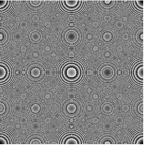
3.4.1 Gray level picture of the function f (m, n) = m2+ n2 mod 419 . . . . 40
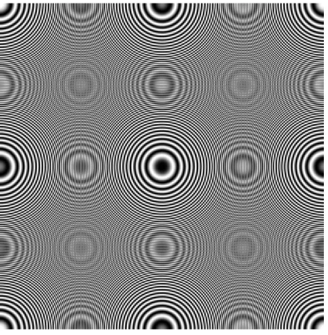
3.4.2 Gray level picture of the function f (m, n) = cos(2π(m2+ n2)/419) . . 41
List of Tables
2.2.1 The expressions for the discrete properties . . . 14 2.2.2 A comparison of the properties of the discrete Wigner distributions
WDm, WDh, WDs. . . 15
3.4.1 Properties of the discrete fractional Fourier transform. . . 36
Introduction
1.1
Wigner distributions
The Wigner Distribution (WD) [1–4] is an important time-frequency representation [5–9]. It is widely used in signal analysis and processing [10], optics [11–13], and quantum mechanics [14]. A discrete-time discrete-frequency version of the WD is of great importance not only for digital signal processing but also for the other fields where the WD is utilized. In defining the discrete version of any transform or representation there are usually two distinct objectives:
• Structural analogy: The discrete entity should satisfy as many operational
properties and relationships analogous to the continuous entity as possible.
• Approximation and limits: The discrete entity should approximate the
samples of the continuous entity and/or the continuous entity should in some sense be the limit of the discrete entity.
The discrete Fourier transform (DFT) satisfies both of these objectives to a very high degree. Most approaches to designing the discrete WD in the literature have primarily emphasized either of the above objectives. Ideally we would desire our definition of the discrete WD also to satisfy both of these objectives. Unfortunately,
CHAPTER 1. INTRODUCTION 2
a definition satisfying both objectives to the same degree as the DFT does not exist. In fact, these two objectives often seem to contradict each other and a trade-off is often necessary. Therefore it is desirable to understand to what extent these objectives can be simultaneously met and the nature of the trade-off between them. For instance, to define the discrete WD so that it exhibits the largest possible structural analogy to the continuous case, it is possible to base its definition in group representation theory in a manner completely analogous to the definition of the continuous WD [15, 16]. Such a definition, referred to as WDmin this thesis,
indeed exhibits a high degree of structural analogy, but fails to approximate the continuous Wigner distribution. In fact, rather convincing arguments have been put forth that WDmis the definition exhibiting the greatest possible degree of structural
similarity, in the sense that this is the only definition which satisfies the discrete versions of a set of properties of the continuous WD that uniquely define it among other members of Cohen’s class [17]. On the other hand, definitions obtained by sampling the continuous WD [3], such as the definition that will be referred to as WDsin this thesis, while approximating the continuous WD, exhibit only a very
limited degree of structural analogy and lack several of the fundamental properties that distinguish the WD from other members of Cohen’s Class. In this thesis we will also study a third definition [18], referred to as WDh, which not only provides a
good continuous approximation, but also exhibits a high degree of structural analogy, and therefore seems to be one of the most desirable definitions of the discrete WD for most purposes. In most respects, the relationship between this definition and the continuous WD, comes closest to the relationship between the DFT and the continuous FT.
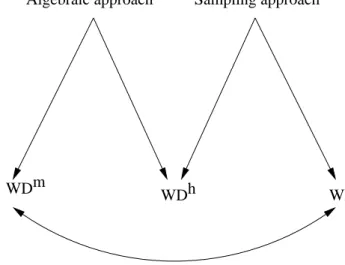
In section 2.1, the derivation of the continuous WD based on the Weyl corre-spondence will be reviewed and this approach will be adapted to the discrete case. Based on how we choose to handle divisions by 2, this leads to the definitions of the discrete WD we refer to as WDmor WDh. Such algebraic approaches lead to
defini-tions exhibiting a high degree of structural analogy to the continuous case (left hand of figure 1.1.1). In section 2.2 the properties of the three discrete WDs discussed in this thesis will be compared. Section 2.3 discusses definitions of the discrete WD
Algebraic approach Sampling approach
WD m WDh WDs
Figure 1.1.1: Approaches to defining the discrete WD and resulting definitions. based on sampling (which achieve continuous approximation), and leads to the defi-nitions we refer to as WDhand WDs(right hand of figure 1.1.1). As we can see from
figure 1.1.1, WDhemerges at the intersection of the algebraic approach which leads
to high structural analogy, and the sampling approach which leads to continuous approximation, and therefore stands out as a definition which satisfies both of our goals to a very high degree. The relationship between WDmand WDsrepresented
by the arc at the bottom of the figure is also discussed in the same section. In section 2.4 a brief discussion of some of the issues from the perspective of group theory will be presented.
The review of the literature has been postponed to section 2.5.
1.2
Linear canonical transforms
The linear canonical transforms (LCT) play an important role in optics, quantum mechanics and also found applications in signal processing [11]. The fractional Fourier transform (FrFT), as a special linear canonical transform, is widely studied in optics [13]. The FrFT and its close relationship with the WD have led to many applications in time-frequency analysis [8]. Defining the discrete versions of these
CHAPTER 1. INTRODUCTION 4
transforms is also important for the fields where the continuous version is used. As with the case of WDs, in the definition of the discrete LCTs we will focus on:
• Structural analogy: The discrete entity should satisfy as many analogous
operational properties and relationships to the continuous entity as possible.
• Approximation and limits: The discrete entity should approximate the
samples of the continuous entity and/or the continuous entity should in some sense be the limit of the discrete entity.
Before proceeding to the discrete analogy we must note the most desirable ob-jective. It would be good to have operators both form a matrix group1 SL(2, R)
and act on a finite dimensional Hilbert space. However, it is stated in [13] pp. 277 that “the group Mp(2, R) has no finite-dimensional matrix representation”. In the literature there has been various proposals for the computation of the LCTs and as a special case the fractional Fourier transform (FrFT) [11]. However these approaches lack structural analogy and desirable properties that designate the LCTs.
It is possible to construct LCTs in a modulo sense where the matrix group becomes SL(2, Zp) and the real field R is replaced with Zp. The field Zp denotes the
integers in [0, p − 1] with the group operations being additions and multiplications in mod p. The representation theory of this group was studied first by Tanaka [19] in an abstract manner. An explicit construction of the metaplectic representation in the Weyl-Fourier form is given in [20–22]. The limits of the discrete metaplectic representation are studied and it is known2 that the discrete LCTs do not have
the continuous LCTs as limits [23]. We will show in section 3.3 that under certain assumptions it is possible to relate the LCTs coming from SL(2, Zp) the continuous
LCTs obtained from SL(2, R).
The fractional Fourier transform is of special interest among the subgroups of
SL(2, R). In section 3.4, we will also study fractional Fourier transforms obtained
from SL(2, Zp) and derive their properties and connections with WDm. Although
1Up to ±1 sign uncertainty
the first studies on the group SL(2, Zp) date back to sixties, to the best our
knowl-edge the discrete FrFT obtained from SO(2, Zp) is not studied in this detail. Authors
of [16, 24] came close to defining the discrete versions of this dicrete FrFT however they do prove many of the properties given in table 3.4.1 and do not write the transform kernel in the complete form that will be presented in 3.4.
A detailed review of the literature and further discussions is postponed to section 3.3.
Chapter 2
Wigner distributions
2.1
Weyl correspondence approach to defining
discrete Wigner distributions
Before defining discrete WDs, we will briefly review the development of the con-tinuous WD based on the Weyl correspondence, an approach also known as the characteristic function operator method [6]. Our inner product convention is
hf, gi =R−∞∞ f (u)g∗(u) du. The Fourier transform is defined as
F{f (u)} = F (µ) =
Z ∞
−∞
f (u)e−j2πµudu, (2.1.1)
F−1{F (µ)} = f (u) =
Z ∞
−∞
F (µ)ej2πµudµ, (2.1.2)
and the coordinate multiplication and differentiation operators are defined as
Uf (u) = uf (u), in the time domain, (2.1.3)
DF (µ) = µF (µ), in the frequency domain, (2.1.4)
where U and D are related through D = F−1UF. Exponentiation of these operators
yields the time-shift and frequency-shift operators. Expressed in the time domain:
ej2π ¯µUf (u) = ej2π ¯µuf (u), (2.1.5)
ej2π ¯uDf (u) = f (u + ¯u). (2.1.6)
We now apply the correspondence principle u → U, µ → D to the function
ej2π(¯µu+¯uµ). This is known as the Weyl correspondence1:
ej2π(¯µu+¯uµ) → ej2π(¯µU+¯uD). (2.1.7)
The entity on the right-hand side will be denoted by ρ(¯u, ¯µ), and can be put in the
following form by employing the Baker-Campbell-Hausdorff formula [11] eA+B =
eAeBe−[A,B]/2 which holds when [A, [A, B]] = [B, [A, B]] = 0 (which is true in our
case since [U, D] = UD − DU = 2πj I):
ρ(¯u, ¯µ) = ej2π(¯µU+¯uD) = ejπ ¯u¯µej2π ¯µUej2π ¯uD
= e−jπ ¯u¯µej2π ¯uDej2π ¯µU. (2.1.8)
With reference to equations (2.1.5) and (2.1.6), ρ(¯u, ¯µ) is an operator with the
effect of combined time and frequency shifting with time-frequency shift parameters ¯
u, ¯µ. Applying this combined shift operator to a function f (u) and taking the inner
product of the result with f (u) yields the correlative time-frequency representation known as the ambiguity function:
Af(¯u, −¯µ) = hρ(¯u, ¯µ)f, f i. (2.1.9)
The Wigner distribution can be defined as the two-dimensional Fourier transform of the ambiguity function:
Wf(u, µ) = Z ∞ −∞ Z ∞ −∞ hρ(¯u, ¯µ)f, f ie−j2π(u¯µ+µ¯u)d¯u d¯µ. (2.1.10)
The above definitions can be easily put in the following forms:
Wf(u, µ) =
Z ∞
−∞
f (u + ¯u/2)f∗(u − ¯u/2)e−j2π ¯uµd¯u, (2.1.11)
= Z ∞ −∞ F (µ + ¯µ/2)F∗(µ − ¯µ/2)ej2π ¯µud¯µ, (2.1.12) Af(¯u, ¯µ) = Z ∞ −∞
f (u + ¯u/2)f∗(u − ¯u/2)e−j2π ¯µudu, (2.1.13)
= Z ∞
−∞
F (µ + ¯µ/2)F∗(µ − ¯µ/2)ej2π ¯uµdµ. (2.1.14)
1We note that the Weyl correspondence, the Schr¨odinger representation of Heisenberg group,
CHAPTER 2. WIGNER DISTRIBUTIONS 8
After this review, two definitions of the discrete WD will be developed in a unified manner. In order to arrive at definitions of the WD which are analogous to the continuous definition in a fundamental sense, we will try to follow the same procedure for defining the continuous WD outlined in the previous section. This is in contrast to approaches based on sampling the continuous WD to arrive at a discrete definition [25–27]
We will be dealing with the discrete index sets S1, S2 respectively:
S1 = {0, 1, 2, 3, . . . , N − 1}, (2.1.15) S2 = n − N − 1 2 , − N − 3 2 , . . . , N − 3 2 , N − 1 2 o , (2.1.16)
where N is odd. Our inner product convention is hf, gi =Pn∈Sf [n]g∗[n]. The DFT
is defined as F{f [n]} = F [k] =X n∈S f [n]e−j2πkn/N, (2.1.17) F−1{F [k]} = f [n] = 1 N X k∈S F [k]ej2πkn/N, (2.1.18)
where S denotes S1 or S2. Which index set is being used will be evident from the
context.
The discrete versions of the coordinate multiplication and coordinate differenti-ation operators can be defined easily [28–30]:
Uf [n] = nf [n], in the time domain, (2.1.19) DF [k] = kF [k], in the frequency domain, (2.1.20) and are related through the DFT: D = F−1UF. Analogous to the continuous case,
we also have [28, 29],
ej2π¯NkUf [n] = e j2π¯kn
N f [n], (2.1.21)
ej2π ¯NnDf [n] = f [n + ¯n]. (2.1.22) Now, we may again analogously introduce the Weyl correspondence as [29]
with the intent of defining a discrete WD in a manner completely analogous to the definition of the continuous WD. However, it is not possible to proceed from this point onward in a completely analogous manner because unlike the continuous case, [U, [U, D]] 6= 0, [D, [U, D]] 6= 0, [U, D]] 6= I, so that we cannot apply an analogous Baker-Campbell-Hausdorff formula. For this reason it has not been possible to define a discrete WD though the Weyl correspondence [29], although the authors did not refer to this obstacle. Furthermore, this outcome is not dependent on the particular definition of U and D chosen, since the commutation relation [U, D] = 2πj I does not
have an analog in the discrete case for any U and D due to the following result [31]: Proposition 1 Two matrices A, B cannot have identity as the commutator: [A, B] = AB − BA 6= I.
proof : Assume that there exists matrices A, B such that AB − BA = I and
take the trace of both sides T r[AB]−T r[BA] = T r[I]. This leads to a contradiction since T r[AB] − T r[BA] = 0 6= T r[I]. ¥
This break of analogy with the continuous case, is a strong indication of the different nature of the discrete scenario. Despite this setback, we will proceed by maintaining the analogy as much as possible by employing the following discrete versions of equation (2.1.8) as two alternative definitions of ρ[¯n, ¯k]:
ρ(¯u, ¯µ) = ejπ ¯u¯µej2π ¯µUej2π ¯uD = e−jπ ¯u¯µej2π ¯uDej2π ¯µU, (2.1.24)
ρm[¯n, ¯k] = ej2π ¯n¯Nk2−1e j2π¯kU N e j2π ¯nD N = e −j2π ¯n¯k2−1 N e j2π ¯nD N e j2π¯kU N , (2.1.25) ρh[¯n, ¯k] = ejπ ¯Nn¯kej2π¯NkUej2π ¯NnD = e−jπ ¯Nn¯kej2π ¯NnDej2π¯NkU. (2.1.26)
Two alternative definitions emerge from the two possible ways of handling the di-vision by 2, both of which have their own advantages. In the first case (2.1.25), 2−1 denotes the mod N inverse of 2 which is given by (N + 1)/2. In the second
case (2.1.26), the division is handled in the usual sense so that 2−1 cancels the 2
in the numerator. Notice that the exponentials are both square roots of the same expression: ej2π ¯Nn¯k = ³ ejπ ¯Nn¯k ´2 = ³ ej2πN [¯n¯k2−1] ´2 . (2.1.27)
CHAPTER 2. WIGNER DISTRIBUTIONS 10
The corresponding WDs may now be written in analogy with the continuous case as: Wf(u, µ) = Z ∞ −∞ Z ∞ −∞ hρ(¯u, ¯µ)f, f i e−j2π(u¯µ+µ¯u)d¯u d¯µ, (2.1.28) Wfm[n, k] = 1 N X ¯ n∈S1 X ¯ k∈S1 hρm[¯n, ¯k]f, f i e−j2π(n¯k+k¯n)/N, (2.1.29) Wfh[n, k] = 1 N X ¯ n∈S2 X ¯ k∈S2 hρh[¯n, ¯k]f, f i e−j2π(n¯k+k¯n)/N. (2.1.30)
Both of these discrete definitions have been studied extensively and originate from [15] and [18] respectively.
Although it is impossible to obtain a discrete WD exactly the same way in the continuous case, we must note that the presented derivation is equivalent to starting with the discrete Rihaczek distribution [29] and then proceeding to the discrete WD. This is still legitimate in the framework of the characteristic function operator method since we can obtain any member of the Cohen’s class from the other members [5].
A third definition of the discrete WD, which we will refer to as WDs, will be
discussed in section 2.3.
2.2
Discussion of the properties of the two WDs
In this section we will compare the two discrete WDs defined in the previous sec-tion. As already noted, WDmis the definition exhibiting the greatest possible degree
of structural analogy but lacks a direct connection to the continuous WD. While WDhdoes not satisfy all the analogous properties of WDm, it approximates the
samples of the continuous WD.
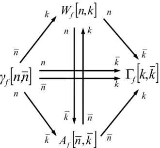
When we speak of structural analogy, we will focus our attention on both op-erational time-frequency properties (look ahead to table 2.2.1) and a set of cross relationships between the WD, the ambiguity function and a set of so-called auxil-iary functions (look ahead to figure 2.2.1) satisfied by the continuous WD.
2.2.1
Auxilary functions
The following auxiliary functions play an important role in the study of the contin-uous WD:
γf(u, ¯u) = f (u + ¯u/2)f∗(u − ¯u/2), (2.2.1)
Γf(µ, ¯µ) = F (µ + ¯µ/2)F
∗(µ − ¯µ/2). (2.2.2)
To define the discrete counterparts of these entities, we must decide how to handle the division by two. For WDmwe define:
γfm[n, ¯n] = f [n + ¯n2−1]f∗[n − ¯n2−1], (2.2.3)
Γmf [k, ¯k] = F [k + ¯k2−1]F∗[k − ¯k2−1], (2.2.4)
where 2−1 is defined in the modulo sense and n + 2−1 is the halfway between n and
n + 1 in a circular context.
Figure 2.2.1 shows the relationships between the discrete WD, ambiguity function and auxiliary functions, which is fully analogous to a similar set of relationships satisfied by their continuous counterparts. The derivation of these relationships are elementary and fully analogous to the derivations in the continuous case and only the derivations of a subset is shown below. First note that the inner product in the definition of the WDmin equation (2.1.29) can be further simplified by a change of
variables n → n − ¯n2−1 as follows: hρm[¯n, ¯k]f, f i = N −1X n=0 ej2π(2−1n¯¯k)/Nej2π¯k(n−¯n2−1)/Nf [n − ¯n2−1+ ¯n]f∗[n − ¯n2−1], = N −1X n=0 f [n + ¯n2−1]f∗[n − ¯n2−1]ej2π¯kn/N. (2.2.5)
CHAPTER 2. WIGNER DISTRIBUTIONS 12 obtained as: Wfm[n, k] = 1 N N −1 X ¯ n,¯k,n0=0 γfm[n0, ¯n]ej2π¯kn0/N e−j2π(n¯k+k¯n)/N = N −1X ¯ n,n0=0 γfm[n0, ¯n]e−j2πk¯n/Nδ[n − n0] = N −1X ¯ n=0 f [n + ¯n2−1]f∗[n − ¯n2−1]e−j2πk¯n/N, (2.2.6)
Equations (2.2.5), (2.2.6) and a corresponding pair of equations for Γf which can
be similarly derived, can be summarized in graphical form (figure 2.2.1) which is familiar from the continuous case [10, 11]. This constitutes further support for the strong structural analogy of this definition to the continuous case. To the best of our knowledge the auxiliary functions have not been defined for WDmand the
relationships depicted in this figure have not been shown.
We now turn our attention to obtaining similar results for WDh. Since division
by two is actually treated as a half-integer in this case, we must more carefully exam-ine the concept of shifting discrete functions by half an integer, since such functions are undefined for non-integer values. Since the operator ej2π ¯NnD corresponds to a shift by the integer amount ¯n, we define a half-integer shift as ejπ ¯NnD = F−1e
jπ ¯nU N F. Applying this operator to a periodic signal f [n] defined over the set S2 we obtain
ejπ ¯NnDf [n] = X n0∈S2 f [n0]φ(n + n¯ 2 − n 0) (2.2.7) where φ(u) = 1 N X n0∈S2 ej2πn0u/N = sin(πu) N sin(πu/N) (2.2.8)
which is essentially an interpolation relation. Note that φ(u), the periodically repli-cated version of the sinc function, is the interpolation function for periodic band-limited signals [32, 33]. When the argument of φ(u) is an integer n, it reduces to φ(n) = δ[n]. Thus φ(u) is a generalization of the delta function and basis to non-integer values.
and (2.2.2) for WDhas follows: ˆ γf[n, ¯n] , ³ ejπ ¯NnDf [n] ´³ e−jπ ¯NnDf∗[n] ´ , (2.2.9) ˆ Γf[k, ¯k] , ³ ejπ¯NkDF [k] ´³ e−jπ¯NkDF∗[k] ´ . (2.2.10)
Unfortunately, these two definitions are neither consistent with each other nor do they lead to a set of relationships of the form given by figure 2.2.1 [34]. The un-derlying reason for this is that fractional shifts as defined above are not distributive over multiplication: ejπ ¯NnD ³ f [n]g[n] ´ 6= ³ ejπ ¯NnDf [n] ´³ ejπ ¯NnDg[n] ´ . (2.2.11)
This can be solved by defining the auxilary functions in asymmetric form [34]:
γfh[n, ¯n] = e−jπ ¯NnD ³ f [n + ¯n]f∗[n] ´ (2.2.12) = ejπ ¯NnD ³ f [n]f∗[n − ¯n]´, (2.2.13) Γhf[k, ¯k] = e−jπ¯NkD ³ F [k + ¯k]F∗[k]´ (2.2.14) = ejπ¯NkD ³ F [k]F∗[k − ¯k]´. (2.2.15)
We reemphasize that due to a lack of the multiplicity property above, these cannot be reduced to the form of equations (2.2.9) and (2.2.10). Nevertheless, in a certain sense these definitions are not so asymmetric since the asymmetric functions f [n + ¯n]f∗[n]
and F [k + ¯k]F∗[k] are symmetrized by applying the operators e−jπ ¯NnD and e−jπ¯NkD
respectively. These definitions fully satisfy the relationships embodied in figure 2.2.1 [34].
2.2.2
Operational properties
In table 2.2.1 we list various properties which a discrete Wigner distribution may be expected to satisfy for both WDmand WDhwhich we have discussed above, and
also for WDswhich we will discuss in a following section.
Properties involving the instantaneous frequency are not included since these do not generalize easily to the discrete-time discrete-frequency case. Also excluded
CHAPTER 2. WIGNER DISTRIBUTIONS 14
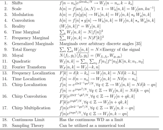
Table 2.2.1: The expressions for the discrete properties
1. Shifts f [n − no]ej2πnko/N → Wf[n − no, k − ko]
2. Scale h[n] = f [an], (a, N ) = 1 → Wh[n, k] = Wf[an, ka−1]
3. Modulation h[n] = f [n]g[n] → Wh[n, k] = Wf[n, k] ?kWg[n, k]
4. Convolution h[n] = f [n] ? g[n] → Wh[n, k] = Wf[n, k] ?nWg[n, k]
5. Reality (Wf[n, k])∗ = Wf[n, k]
6. Time Marginal PkWf[n, k] = N|f [n]|2
7. Frequency Marginal PnWf[n, k] = N|F [k]|2
8. Generalized Marginals Marginals over arbitrary discrete angles [35] 9. Total Energy PnPkWf[n, k] = N×Energy of the signal
10. Moyal Nhf1, g1ihf2, g2i = hWf1,f2, Wg1,g2i 11. Quadratic Wf[n, k] = P n1 P n2f [n1]f ∗[n 2]K[n, k; n1, n2] 12. Fourier Transform WF[n, k] = Wf[−k, n] 13. Frequency Localization F [k] = δ[k − ko] → Wf[n, k] = Nδ[k − ko] 14. Time Localization f [n] = δ[n − no] → Wf[n, k] = Nδ[n − no] 15. Chirp Localization f [n] = ej2π2−1qn2/N , ∀q ∈ Z → Wf[n, k] = Nδ[k − qn] f [n] = ejπqn2/N , ∀q ∈ Z → Wf[n, k] = Nδ[k − qn]
16. Chirp Convolution F [k]ej2π2−1qk2/N
, ∀q ∈ Z → Wf[n + qk, k]
F [k]ejπqk2/N
, ∀q ∈ Z → Wf[n + qk, k]
17. Chirp Multiplication f [n]ej2π2−1qn2/N
, ∀q ∈ Z → Wf[n, k − qn]
f [n]ejπqn2/N
, ∀q ∈ Z → Wf[n, k − qn]
18. Continuous Limit Has the continuous WD as a limit 19. Sampling Theory Can be utilized as a numerical tool
∗All summations are carried out over one period N (N is odd). ‡All inversions are performed in mod N.
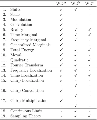
Table 2.2.2: A comparison of the properties of the discrete Wigner distributions WDm, WDh, WDs. WDm WDh WDs 1. Shifts X X -2. Scale X - -3. Modulation X - -4. Convolution X - -5. Reality X X X 6. Time Marginal X X X 7. Frequency Marginal X X -8. Generalized Marginals X - -9. Total Energy X X X 10. Moyal X X -11. Quadratic X X X 12. Fourier Transform X X -13. Frequency Localization X X -14. Time Localization X X X 15. Chirp Localization X - -- X -16. Chirp Convolution X - -- X -17. Chirp Multiplication X - -- X -18. Continuous Limit - X -19. Sampling Theory - X X
CHAPTER 2. WIGNER DISTRIBUTIONS 16
Figure 2.2.1: Graphical representation of the relationships between the two WDs, their corresponding ambiguity functions and auxiliary functions. The relationships are valid for both WDmand WDh. Arrows denote DFTs.
are finite time support and finite frequency support properties due to difficulties in defining them in the cyclic case.
As noted in the introduction, WDmsatisfies all of the structural properties
satis-fied by the continuous WD, with the exception of those which have a meaning only in the continuous case. This is a consequence of the fact that WDmand the continuous
WD are two different realizations of the same underlying group-theoretical structure. Compared with WDm, we observe that the most important properties WDhlacks
are the convolution and modulation properties. On the other hand, WDmlacks a
direct relationship to the continuous WD in the sense of sampling or approxima-tion. As noted in [16], WDmsatisfies chirp multiplication and convolution properties
(properties 15, 16) for modulo chirps ej2π(2−1qn2)/N
. However, these chirps are equal to common chirp functions only when q is even but not when q is odd:
ej2π(2−1qn2)/N
6= ejπqn2/N
, q is odd. (2.2.16)
Most of the properties in table 2.2.2 are either known or can be verified easily and are omitted. Properties 14, 15, 16 are derived for WDmin [24]; here we sketch
the derivation for WDh. Although we cannot use the chirp ejπqn2/N
directly in the definition of WDhsince it is not periodic with N, we can still prove property 15.
Lets assume that the following equality holds for the WDs of two signals g and h.
Wgh[n, k] = Wfh[n, k − qn], (2.2.17)
from this we can infer that
γgh[n, ¯n] = γfh[n, ¯n]ej2πqn¯n/N. (2.2.18)
Applying the ejπ ¯NnD operator to both sides gives2
g[n + ¯n]g∗[n] = f [n + ¯n]f∗[n]ej2πq(n+¯n/2)¯n/N. (2.2.19)
Now letting n = 0,
g[¯n]g∗[0] = f [¯n]f∗[0]ejπq¯n2/N
, (2.2.20)
from which we conclude that the effect of chirp multiplication is shearing in the frequency direction. The other chirp properties 14, 16 can be derived in a similar manner.
Several sets of desirable properties that uniquely define the continuous WD have been proposed. First we consider the set of properties consisting of properties 1, 3-4, 5, 10, 11 in table 2.2.1. In [17] it is shown that the only discrete distribution satisfying all of these properties is WDmand that only for odd values of N.
Within this framework we now summarize our comparison of WDmand WDh.
The use of WDhentails a loss of a number of structural properties compared to
WDm, most prominent of which are the convolution and multiplication
proper-ties. However, since WDmcannot be directly related to the continuous WD, which
severely limits its usefulness in many applications, and since WDmis the only
defini-tion satisfying all of properties 1, 3-4, 5, 10, 11, in seeking an alternative definidefini-tion it necessarily follows that we must lose at least one of these properties. Given the importance of these properties, the convolution and multiplication properties seem the most dispensable, despite their attractiveness. It is also interesting to note that the modulation and convolution properties are virtually absent from the physics literature on finite phase-space theory despite the fact that they are common in the
2Despite the fact that the fractional shift operator is not multiplicative in general, it is so if one
CHAPTER 2. WIGNER DISTRIBUTIONS 18
signal processing literature. Turning our attention to the property of generalized marginals, once again in seeking an alternative definition we must abandon this property.
While we are not able to similarly argue for the inevitable loss of the scaling property 2 for WDh, we note that this property is satisfied by WDmonly for prime
values of N and it does not seem to be considered among the most important properties of the WD, as also evidenced by the lack of its appearance in the above mentioned sets of essential properties. On the other hand, WDhcan be related to the
continuous WD in the sense of sampling or approximation, and the chirps involved in the chirp multiplication and convolution properties are analogous to continuous chirps, neither of which is true for WDm.
It is also of interest to consider another set of properties uniquely defining the continuous WD. It is known that the only member of Cohen’s class of time-frequency distribution satisfying property 14 in the continuous case is the continuous WD [36]. Although we do not give any proof in the discrete case, it is quite possible that the discrete versions of chirp localization properties uniquely define the discrete WDs in the discrete case. In this perspective the definition WDhseems better than
WDmsince it has the localization property with the common chirp signal ejπqn2/N while WDmhas the localization property with the modulo chirp signal ej2π2−1qn2/N
. Therefore, all things considered, WDhemerges as a definition of the discrete
WD which can be used to approximate the continuous WD or related to it through sampling, and at the same time, has a group-theoretical foundation, and satisfies a large number of structural properties. The few properties it does not satisfy seem to be more or less the most dispensable ones among those which cannot be all simultaneously satisfied. As a result, this definition seems to be a very strong, if not the strongest candidate for a Wigner distribution combining the two major objectives set out in the introduction of this chapter.
2.3
Connections to the continuum and sampling
The discrete Fourier transform (DFT) satisfies both of the major objectives set out in the introduction, namely structural analogy and numerical approximation of the the continuous Fourier transform. As already stated, ideally we would like to achieve the same with our definition of the discrete Wigner distribution. The definition WDmalready discussed in detail, satisfies a maximal set of properties analogous to
the continuous WD, but cannot be used to approximate the continuous WD, and thus completely fails to satisfy one of our objectives despite it elegance.
In this section we first consider a widely used definition for the discrete WD, which is widely used for computational purposes [8, 37]:
Ws f(n, k) = M −1X ¯ n=0 f (n + ¯n)f∗(n − ¯n)e−j2π¯nk/M. (2.3.1)
In the above definition, f (n) denotes the samples of the signal which has duration
M. The shifts inside the summation are linear and not cyclic. This definition avoids
aliasing if the sampling rates are double the Nyquist rate. As shown in table 2.2.2, this definition fails to satisfy many of the desirable properties expected of a defi-nition of the discrete WD. Therefore, despite its useful relation to the continuous WD, this definition fails to satisfy our objective regarding structural analogy to the continuous WD. Since our aim is to satisfy both of the objectives of continuous approximation and structural analogy, even if to a limited extent, the definitions WDmand WDscannot be rated very highly since they do very poorly in the first
and second of our objectives respectively.
Furthermore, we also note that WDsis not fully analogous to the continuous WD
in a formal sense either due to the absence of the 1/2 terms in the arguments of the functions.
2.3.1
Sampling and WD
hIn this section we will give a derivation of the definition WDhbased on sampling
CHAPTER 2. WIGNER DISTRIBUTIONS 20
[−∆u/2, ∆u/2] in the time domain and [−∆µ/2, ∆µ/2] in the frequency domain. Under this assumption, the WD of the signal is confined to a region [−∆u/2, ∆u/2]× [−∆µ/2, ∆µ/2], and the AF is confined to a region [−∆u, ∆u] × [−∆µ, ∆µ] due to the correlative nature [11]. Thus, the energy of the signal can be approximated as:
Energy of the signal ≈ Z ∆u 2 −∆u 2 Z ∆µ 2 −∆µ 2 Wf(u, µ) du dµ. (2.3.2)
By proper choice of ∆u and ∆µ, this approximation can be made as accurate as necessary. In order to obtain a discrete WD by sampling the continuous WD, we will use the relationship between the WD and the AF and then the definition of the ambiguity function in terms of auxiliary functions. Since there are four parameters
u, ¯u, µ, ¯µ there will be four corresponding sampling rates, respectively Tu, Tu¯, Tµ, Tµ¯.
These sampling rates must be chosen in such a way that there is no aliasing and the structural relationships inherent in figure 2.2.1 are maintained. Since the WD is the double Fourier transform of the AF, and both are confined to a finite region, we can apply the sampling theorem and use a double DFT to compute the samples of the WD from the samples of the AF. The continuous WD and AF are related as follows: Wf(u, µ) = Z ∞ −∞ Z ∞ −∞
Af(¯u, −¯µ)e−j2π(u¯µ+¯uµ)d¯u d¯µ. (2.3.3)
We will use the asymmetric form of the AF obtained by the variable substitution
u → u + ¯u/2 for sampling:
Af(¯u, −¯µ) = ejπ ¯u¯µ
Z ∞
−∞
ψ(u, ¯u)ej2πu¯µdu. (2.3.4)
= e−jπ ¯u¯µ
Z ∞
−∞
Ψ(µ, ¯µ)ej2π ¯uµdµ. (2.3.5)
where ψ(u, ¯u) = f (u + ¯u)f∗(u) and Ψ(µ, ¯µ) = F (µ − ¯µ)F∗(µ). The samples of the
AF are Af(¯nTu¯, −¯kTµ¯) = ejπ¯n¯kTµ¯Tu¯ Z ∞ −∞ ψ(u, ¯nT¯u)ej2πu¯kTµ¯du (2.3.6) = e−jπ¯n¯kTµ¯T¯u Z ∞ −∞ Ψ(µ, ¯kTµ¯)ej2π¯nTu¯µdµ. (2.3.7)
In order to avoid aliasing in the WD domain, the following conditions must be satisfied 1 Tu¯ ≥ ∆µ, 1 Tµ¯
≥ ∆u, Sampling the AF, (2.3.8)
1
Tu
≥ 2∆µ, 1
Tµ
≥ 2∆u, Sampling the WD. (2.3.9)
Returning to equation (2.3.6) and (2.3.7) which give the samples of the AF, they are still expressed in terms of continuous functions. To replace the Fourier transform of ψ(u, ¯nTu¯) and Ψ(µ, ¯kTµ¯) with an inverse DFT, we must observe the following
relationships to avoid aliasing: 1
Tu
≥ 2∆µ, 1
Tµ¯
≥ ∆u, Constraints for eq. (2.3.6) (2.3.10)
1
Tµ
≥ 2∆u, 1
Tu¯
≥ ∆µ Constraints for eq. (2.3.7) (2.3.11) due to the quadratic structure of ψ(u, ¯nTu¯) and Ψ(µ, ¯kTµ¯). Note that (2.3.10),
(2.3.11) are consistent with the (2.3.8), (2.3.9) set of constraints. The samples of the AF (2.3.6), (2.3.7) will be approximated as:
Af(¯nTu¯, −¯kTµ¯) ≈ ejπ¯n¯kTµ¯Tu¯ X n ψ(nTu, ¯nTu¯)ej2πn¯kTuTµ¯ (2.3.12) Af(¯nT¯u, −¯kTµ¯) ≈ ejπ¯n¯kTµ¯Tu¯ X k Ψ(kTµ, ¯kTµ¯)ej2πn¯kTu¯Tµ (2.3.13)
We must choose the sampling rates Tu, Tu¯, Tµ, Tµ¯ such that there is no aliasing and
the definition WDhis obtained. We shall choose,
Tu¯Tµ¯ = TuTµ¯ =⇒ T¯u = Tu, (2.3.14)
T¯uTµ¯ = Tu¯Tµ=⇒ Tµ¯ = Tµ. (2.3.15)
This choice is necessary since the term ejπ¯n¯kTµ¯Tu¯ and ej2πn¯kTuTµ¯ in equation (2.3.12) must have equal periods. With these assumptions on the sampling rates, the asym-metric auxiliary functions can be written as:
ψ(nTu, ¯nTu¯) = f (nTu + ¯nTu¯)f∗(nTu) → f (n + ¯n)f∗(n), (2.3.16)
CHAPTER 2. WIGNER DISTRIBUTIONS 22
If we combine the constraints in equations (2.3.8), (2.3.9), (2.3.10), (2.3.11) and (2.3.14), (2.3.15) the following rates are the minimum ones:
Tu = Tu¯ =
1
24µ, Tµ= Tµ¯ = 1
24u. (2.3.18)
However, if we further assume that ∆u∆µ is chosen such that ∆u∆µ = N integer, then the optimal choice leads to 4N length DFTs. Unfortunately, the definition WDhis defined only for odd length signals and as a result we can not obtain WDhin
this optimal sampling strategy. In order to have an odd length WD, we will choose the following sampling rates:
Tu = Tu¯ = 1 24µ, Tµ= Tµ¯ = 2∆µ 4∆u∆µ + 1 < 1 2∆u. (2.3.19)
Since f (n) has duration 2N, f (n + ¯n)f∗(n) also has duration 2N. The summation
in 2.3.12 can be put in to the following form:
A(¯nTu¯, −¯kTµ¯) ≈ e jπ ¯n¯k 4N +1 N X n= −N f (n + ¯n)f∗(n)ej2πn¯4N +1k = e4N +1jπ ¯n¯k 2N X n= −2N f (n + ¯n)f∗(n)ej2πn¯4N +1k (2.3.20) By zero padding the 2N nonzero terms in f (n) to 4N + 1, periodically replicating and writing as f [n], the summation can now be written as:
Ahf[¯n, −¯k] = e4N +1jπ ¯n¯k
2N
X
n=−2N
f [n + ¯n]f∗[n]ej2πn¯4N +1k. (2.3.21)
We replaced the linear shifts with circular shifts since the signal f [n] has duration 2N and the correlative shifts in f [n + ¯n]f∗[n] are in the range of ¯n ∈ [−2N, 2N].
Note that we obtained the ambiguity function corresponding to the WDh. Then
the WDhwill be the double DFT of the AFh.
It is also possible to make other choices like:
Tu = Tu¯ = 2∆u 4∆u∆µ + 1 < 1 2∆µ, Tµ= Tµ¯ = 1 2∆u. (2.3.22)
Since F (k) has duration 2N, F (k − ¯k)F∗(k) also has duration 2N. The summation
in 2.3.13 can be put in to the following form:
A(¯nTu¯, −¯kTµ¯) ≈ e jπ ¯n¯k 4N +1 N X k= −N F (k − ¯k)F∗(k)ej2πk¯4N +1n = e jπ ¯n¯k 4N +1 2N X k= −2N F (k − ¯k)F∗(k)ej2πk¯4N +1n (2.3.23)
by zero padding the 2N nonzero terms in F (k) to 4N + 1, periodically replicating and writing as F [k], the summation can now be written as:
Ahf[¯n, −¯k] = e4N +1jπ ¯n¯k
2N
X
k=−2N
F [k − ¯k]F∗[k]ej2πk¯4N +1n. (2.3.24)
We replaced the linear shifts with circular shifts since the signal F [k] has duration 2N and the correlative shifts in F [k − ¯k]F∗[k] are in the range of ¯k ∈ [−2N, 2N].
Note that we obtained the ambiguity function corresponding to the WDh. Then
the WDhwill be the double DFT of the AFh.
In summary, we must sample the signal at twice the Nyquist rate and then apply zero padding such that the final length is 4N + 1 where N denotes the number of degrees of freedom. We made two operations which included redundancy. The first one is sampling at the double Nyquist rate. This is necessary and natural since the AF is quadratic and this results in frequency doubling. We further applied a zero padding which is still necessary since the AF is of correlative nature and in order to replace linear correlation with circular correlation zero padding is necessary.
2.3.2
Relationship between WD
mand WD
sIn this subsection we will show a simple relationship between the definitions WDmand WDsdefined as:
Wfs(n, k) =
M −1X
¯
n=0
f (n + ¯n)f∗(n − ¯n)e−j2π¯nk/M. (2.3.25)
The shifts in above expression are linear. However the definition WDmis defined by
using cyclic shifts. If the signal f (n) is zero padded to N ≥ 4M + 1 and denoted as
f [n], the linear shifts in the definition can be represented with cyclic shifts. WDscan
be written as: Wfs[n, k] = N −1 X ¯ n=0 f [n + ¯n]f∗[n − ¯n]e−j2π¯nk/N. (2.3.26)
CHAPTER 2. WIGNER DISTRIBUTIONS 24
0 1 2 3 4 5 6 7 8 9 10 11 12 13 14
0 1 2 3 4 5 6 7 8 9 10 11 12 13 14
md
hb
Figure 2.3.1: The permutation of the values of WDmand WDsalong the k axis for
N = 15. (md refers to WDmand hb refers to WDs)
Wfm[n, k] = N −1X ¯ n=0 f [n + ¯n2−1]f∗[n − ¯n2−1]e−j2πk¯n/N = N −1X ¯ n=0 f [n + ¯n]f∗[n − ¯n]e−j2π(2¯nk)/N = Wfs[n, 2k], (2.3.27) or equivalently Wfs[n, k] = Wfm[n, 2−1k], (2.3.28)
where 2−1k is again computed modulo N. We used the substitution ¯n → 2¯n in
passing to the second line of (2.3.27). This remarkably simple relationship means that the values of either of these WDs is obtained simply by rearranging (permuting) the values of the other along the frequency axis (figure 2.3.1). It is interesting to note that the resulting permutation is in the form of a perfect shuffle and is also related to decimation in time. This relationship also means that if we know the WD according to one of these definitions, we can quickly compute WD according to the other definition by simply rearranging the values. where f [n] is periodic and the shifts in the definition are cyclic.
2.4
Group theoretical discussion
In this section we will give a group theoretical discussion for the definitions of discrete WDs. We will avoid a detailed and rigorous treatment and will provide a general
sketch of the theory. Before proceeding to a group theoretical foundations of the WD, we will briefly review the definitions of a group, Lie group, differentiable manifold, and Lie algebra. Rigorous definitions and detailed treatment of the subject can be found in [13, 38].
A group is a set associated with a binary operation such that the binary opera-tion defined on this set satisfies closure, existence of identity, existence of an inverse for all members, and associativity properties. The real line with addition operation is a common example of a group. A Lie group has an extra structure in addition to the group property: a differentiable manifold. A differentiable manifold is a general-izations of a differentiable curve to higher dimensions. The real line, the sphere, and the torus are examples of differentiable manifolds. A Lie algebra is a linear space associated with a binary operation called the Lie bracket. A common example of a Lie algebra is the 3 dimensional vector space with the vector product being the Lie bracket. There exists a very important connection between Lie groups and Lie algebras. The Lie algebra is the tangent space of the Lie group near the identity element of the group. Furthermore the exponential map connects one parameter subgroups of a Lie group to the corresponding Lie algebra.
The Heisenberg group is also a Lie group and the members of the group are given as:
ρ(¯u, ¯µ, t) = ej2π(¯µU+¯uD+tI) (2.4.1)
= ej2πtIejπ ¯u¯µej2π ¯µUej2π ¯uD (2.4.2)
where ¯u, ¯µ, t are the 3 parameters of the group. The operator ρ(¯u, ¯µ, t) is usually
called the Schr¨odinger representation of the Heisenberg group. The operator ¯µU +
¯
uD + tI is called the Schr¨odinger representation of the Heisenberg Lie algebra where
the Lie bracket is the commutator of two operators ([U, D] = UD − DU = 2πj I).
The derivation of the continuous WD based on the operator ρ(¯u, ¯µ, t) is presented in
section 2.1. A careful observation of this derivation reveals that the definition of the continuous WD is solely based on the Heisenberg group and the operator given in equation (2.4.2). The transition from equation (2.4.1) to (2.4.2) is not a necessary part of the definition of the continuous WD.
CHAPTER 2. WIGNER DISTRIBUTIONS 26
In order to define a discrete WD distribution in complete analogy to the continu-ous case, all of the ingredients in the continucontinu-ous group theoretical derivation must be replaced with corresponding discrete versions. However it is not possible to extend a differentiable manifold to the discrete case. But the infinite group can be replaced with a finite group in many cases. In the case of the Heisenebrg group it is shown in proposition 1 that the Heisenberg Lie algebra can not be extended to the discrete case since it is impossible to find matrices whose commutator identity. Note that the Weyl correspondence approach written in equation (2.1.7) depends not only on the group structure but also to the Lie algebra which is connected with the differentiable manifold property of the Lie group, since the [U, D] = UD − DU = 2πj I property is
used. The finite analogs of Lie groups that lack the differentiable manifold structure are usually called Lie type groups.
In the discrete case, two realizations of the finite Heisenberg group have been studied.
ρm[¯n, ¯k, τ ] = ej2πτ I/Nej2π2−1n¯¯k/Nej2π¯kU/Nej2π¯nD/N (2.4.3)
ρh[¯n, ¯k, τ ] = ej2πτ I/Nejπ¯n¯k/Nej2π¯kU/Nej2π¯nD/N (2.4.4)
where the parameters ¯n, ¯k, τ ∈ S1 and ¯n, ¯k, τ ∈ S2. The operator ρ
m
is advantageous in the sense that it leads to WDm, which is structurally more analogous to the
continuous WD. The cost for this is the loss of the connection with continuum. On the other hand, ρh leads to WDhand has a connection to continuum. The group
theoretical discussions for ρm can be found in [15,21,24,39,40]. On the other hand ρh was studied in [18, 41] and has the continuous Heisenberg group as a limit [41]. We must note that the theory works best only for prime lengths and to some exceptions for odds for both of the realizations of the finite Heisenebrg group ρm and ρh.
2.5
Review of the literature and discussions
The concept of discrete phase space was first studied by J. von Neumann [42] and later further developed by A. Weil [15]. To the best of our knowledge, J. Schwinger was the first researcher to explicitly study a discrete Weyl correspondence [18].
Detailed and rigorous treatment of the phase space can be found in [14, 38, 43, 44]. As we have mentioned in the introduction, approaches to defining a discrete WD can be categorized as mainly falling under two headings: algebraic approaches and approaches based on sampling. Algebraic approaches based on the Weyl correspon-dence, the Schr¨odinger representation of the Heisenberg group, and the Schwinger basis all essentially lead to the same operators ρm and ρh defined in section 2.1. To the best of our knowledge, the operator ρm is first studied by A. Weil [15] and the operator ρh is first studied by J. Schwinger in [18]. The operator ρm is studied by many authors including [20,21,24,39,45] and the operator ρhis studied by many au-thors including [29,30,41,46] within the context of finite phase space. Wootters [35] independently rediscovered the definition WDmfor prime length signals [47].
Most approaches to defining discrete WDs in the signal processing literature are based on sampling theory [25–27, 48, 49]. The earliest work we are aware of to give such a definition of a discrete WD is [3]. The work of Richman and others [24] is an exception in that it is based on group representation theory. Other works based on algebraic approaches in signal processing are [17, 29]. Sampling theory is adopted by many authors [25, 50] for the implementation and the computation of the WD. Special emphasize is given to computation of the WD without aliasing. Although these approaches lead to successful computational methods for the continuous WD, they lack structural analogy to the continuous WD. A review of sampling theory based approaches can be found in [27]. Other works in signal processing are [49,51]. The definition WDmis studied by [17, 24] in signal processing. To the best of our
knowledge the definition WDhis not studied in the signal processing literature. A
generalization of the Shannon sampling theorem in WD domain is discussed in [52]. One very interesting and unifying approach which leads to a definition which satisfies both of our requirements of structural analogy and numerical approximation is based on the Kravchuk functions. The main motivation comes from the well-established theory in [53], and the associated Wigner distributions are developed in [54]. This approach is supported by its relation to developments involving discrete Gauss-hypergeometric functions [53]. The fundamental drawback of this approach is that it is not consistent with the conventional definition of the DFT, which must be
CHAPTER 2. WIGNER DISTRIBUTIONS 28
replaced with the discrete Kravchuk-Fourier transform [55]. The Kravchuk-Fourier transform also approximate the continuous Fourier transform and is related to the DFT but is not equivalent to it. There has been many attempts to study discrete WDs along these lines [46, 54], but we are unable to judge whether it is desirable or acceptable to give up the conventional DFT.
One of our primary objectives set for the definition of a discrete entity was the continuum limits property. The limits of the finite Heisenberg group and discrete WDs are usually evaluated by comparing with a Reimann sum in the literature. A mathematically rigorous treatment of the limits for discrete operators and finite spaces is discussed in [56, 57] by using inductive resolutions. Inductive resolutions are generalizations of the limits of functions and sequences to groups, spaces and other algebraic entities.
Despite the fact that the WD is extensively used in both signal processing and quantum mechanics, and the many analogies between them, it is used in quite different contexts and forms in these two fields. Nevertheless the similarity between them point to further analogies between the phase spaces of discrete signal analysis and finite quantum mechanics. Finite phase space and discrete WDs are important concepts in the area of quantum computation [58]. However, because the discrete WDs employed in this field are chosen to be of even length, the WDs discussed here may not be of much use. It is worth noting a closely related recent work in processing quantum signals [59]. Other works in finite quantum mechanics and quantum computation literature dealing with the finite phase space are [60–66].
In this thesis we discussed discrete WDs only for the case of odd length signals. This is a consequence of the use of approaches based on structural analogies; even some approaches based on sampling theory have the same structure. The authors of [17] show that a discrete WD exists only for odd lengths, by imposing the analogs of the properties which uniquely define the WD in the continuous case. Indeed WDmsatisfies the generalized marginal properties only for prime length signals [35].
These all show that the parity plays an important role, especially in approaches based on structural analogies. Indeed, the definitions in [24, 45] for even length signals are very different from the ones for odd length signals. There has been
proposals for overcoming these parity issues in defining the discrete WD in a unified manner for odd and even length signals [67]. A distinct definition for even length signals can be found in [68].
Chapter 3
Linear Canonical Transforms
3.1
Continuous linear canonical transforms
In this section, we will briefly review the continuous theory of LCTs and their connection with the WD from [11, 69]. We will avoid a detailed group theoretical discussion since there exists excellent sources on the subject [13, 38, 69] and such an approach may lead us too far away from our purpose. Nevertheless, we will emphasize the differences and similarities of discrete and continuous LCTs in a group theoretical perspective.
The continuous LCTs are defined as: (CMf )(u) = Z ∞ −∞ CM(u, u0)f (u0) du0, (3.1.1) CM(u, u0) = AMejπ(αu 2−2βuu0+γu02) , (3.1.2) AM = p βe−jπ/4. (3.1.3)
There exists an ambiguity in the computation of the square roots in the above definitions. We will use the same convention in [11] which takes the root that falls in (−π/2, π/2]. The parameters α, β, γ are real1, independent and are denoted with
1The complex case is also studied in [69]
M in the above definitions. LCTs can also be written in the following form: CM(u, u0) = AMejπ( D Bu2−B2uu0+ABu02), (3.1.4) AM = √1 Be −jπ/4, (3.1.5) M = " A B C D # , AD − BC = 1. (3.1.6)
The FrFT is a special linear canonical transform corresponding to the rotation subgroup SO(2, R). Fa= ejaπ/4CM (3.1.7) for −2 ≤ a ≤ 2 and M = " cos(πa/2) sin(πa/2) − sin(πa/2) cos(πa/2) # . (3.1.8)
The transform has been studied independently by many authors in different contexts and a detailed review of the literature can be found in [11].
LCTs have the following so called ABCD distortion property on the WD:
WfM(Au + Bµ, Cu + Dµ) = Wf(u, µ), (3.1.9)
where fM = (CMf )(u). As a special case, fractional Fourier transform rotates the
WD.
3.2
Discrete linear canonical transforms
In this section, we will define the discrete versions of LCTs and make connections to continuum. Before making the definitions we will introduce the Gauss sums since they play a major role in the construction. Indeed Gauss sums are the discrete versions of chirp integrals and Fourier transforms of chirps signals that play an important role in the continuous theory [11].
CHAPTER 3. LINEAR CANONICAL TRANSFORMS 32
The Gauss sum Gp for an odd prime p is [70]:
Gp[n] = 1 √ p X m∈Zp ej2πp [nm2]=³n p ´ Gp(1), n 6= 0 (3.2.1) Gp(1) is computed as: Gp(1) = ( 1, p = 1 mod 4; j, p = 3 mod 4. (3.2.2) and (n
p) denotes the Legendre symbol:
³n p ´ = ( 1, n = r2 mod p; −1, n 6= r2 mod p. (3.2.3)
Gauss sums and the Legendre symbol play an important role in number theory [70]. The representation theory of the group SL(2, Zp) was first studied by Tanaka [19]
in an abstract form. An explicit construction of this representation in Weyl-Fourier form is given in [22]. A different but related treatment of the problem is [71]. The discrete LCTs are given in the following form in [23].
(CMf )[n] = X n0∈Zp f [n0]C M[n, n0], (3.2.4) CM[n, n0] = GMe j2π p [2−1B−1(Dn2−2nn0+An02)], (3.2.5) GM = 1 √ pG ∗ p[2B], (3.2.6)
where the parameters A, B, C, D ∈ Zp.
It is stimulating to compare the definitions of continuous and discrete LCTs since they exactly share the same structure. The kernel of the discrete LCTs has the following properties which imply the unitarity of the discrete transform:
C−1
M[n, n0] = CM∗ [n0, n] = CM−1[n, n0]. (3.2.7) The effect on the discrete Wigner distribution WDmcan be easily proved by
making the following matrix decompositions in mod p. " A B C D # = " 1 0 DB−1 1 # " B 0 0 B−1 # " 0 1 −1 0 # " 1 0 AB−1 1 # (3.2.8)
The effect of discrete LCTs on WDmtakes a similar form to the continuous case. Wfm[n, k] = √1 N N −1X ¯ n=0 f [n + ¯n2−1]f∗[n − ¯n2−1]e−j2π¯nk/N (3.2.9) WfmM[An + Bk, Cn + Dk] = Wfm[n, k] (3.2.10)
where fM = (CMf )[n]. The discrete versions of the ABCD distortion for WDmhave
also been shown in [16, 24]. However authors do not give any definition for the discrete LCTs and do not derive the matrix group properties.
3.3
Continuum connections
The discrete LCTs discussed in the previous section are obtained from the theory of the group SL(2, Zp). These discrete LCTs are exactly analogous to the continuous
LCTs in the sense of operational properties. It has also been shown that the discrete LCTs do not have the continuous LCTs as continuous limits [23]. Nevertheless, we will show that it is possible to relate these discrete LCTs to the samples of the continuous LCTs. Thus, with regard to the two main desirable qualities set in the introduction, the discrete LCTs discussed in the previous section exhibit high structural analogy, are not related to continuous LCTs through continuous limits but nevertheless can approximate them under certain conditions.
The discrete versions of chirp signals and their connections to the continuous chirps has been discussed in [72]. It is shown that under certain assumptions it is possible to relate the continuous chirp modulated Fourier transform to the discrete versions. Various optimality and approximation considerations has been derived in [72]. In this section, we will apply the methodology in [72] to relate the continuous LCTs to the discrete LCTs.
CHAPTER 3. LINEAR CANONICAL TRANSFORMS 34
For reference, we rewrite the continuous LCTs: (CMf )(u) = Z CM(u, u0)f (u0) du0, (3.3.1) CM(u, u0) = AMejπ(αu 2−2βuu0+γu02) , (3.3.2) AM= p βe−jπ/4. (3.3.3)
To show the connection between the continuous LCTs and the discrete LCTs, we will approximate the integral in the definition of continuous LCTs as follows:
Z CM(u, u0)f (u0)du0 ≈ X n0 CM(nTu, n0Tu0)f (n0) (3.3.4) where CM(nTu, n0Tu0) = AMejπ(αn 2T2 u−2βnn0TuTu0u0+γn02Tu02), (3.3.5) AM = p βe−jπ/4. (3.3.6)
Note that this approximation is true up to multiplicative constants. We will choose the sampling rates as Tu = Tu0 =
p
2/p, then the sampled kernel takes the following form:
CM(nTu, n0Tu0) = AMej2π(αn
2−2βnn0u0+γn02)/p
. (3.3.7)
If we compare the samples of the kernel with the kernel of discrete LCTs given below:
CM[n, n0] = GMe
j2π
N [2−1B−1(Dn2−2nn0+An02)], (3.3.8) for the following values of the continuous LCTs parameters
α = 2−1B−1D, (3.3.9)
β = 2−1B−1, (3.3.10)
γ = 2−1B−1A, (3.3.11)
the two kernels given in equations (3.3.7) and (3.3.8) become equivalent up to mul-tiplicative constants.
In summary, the approximation property shown above is valid only in a limited context. For a given discrete LCT with parameters A, B, C, D ∈ Zp, there exists a