FINANCIAL DEVELOPMENT AND PRODUCTIVITY A PANEL DATA APPROACH
A Master’s Thesis by BURCU AFYONOĞLU The Department of Economics Bilkent University Ankara June 2006
FINANCIAL DEVELOPMENT AND PRODUCTIVITY A PANEL DATA APPROACH
The Institute of Economics and Social Sciences of
Bilkent University
by
BURCU AFYONOĞLU
In Partial Fulfillment of the Requirements for the Degree of MASTER OF ARTS
in
THE DEPARTMENT OF ECONOMICS BİLKENT UNIVERSITY
ANKARA
I certify that I have read this thesis and have found that it is fully adequate, in scope and in quality, as a thesis for the degree of Master of Arts in Economics.
--- Assoc. Prof. Fatma Taşkın Supervisor
I certify that I have read this thesis and have found that it is fully adequate, in scope and in quality, as a thesis for the degree of Master of Arts in Economics.
--- Asst. Prof. Selin Sayek Böke Examining Committee Member
I certify that I have read this thesis and have found that it is fully adequate, in scope and in quality, as a thesis for the degree of Master of Arts in Economics.
--- Assoc. Prof. Süheyla Özyıldırım Examining Committee Member
Approval of the Institute of Economics and Social Sciences
--- Prof. Erdal Erel
ABSTRACT
FINANCIAL DEVELOPMENT AND PRODUCTIVITY A PANEL DATA APPROACH
Afyonoğlu, Burcu
M.A., Department of Economics Supervisor: Assoc. Prof. Fatma Taşkın
June 2006
Much ink has been spilled over the relation of financial market development and economic growth. Productivity growth is one of the main sources of economic growth. In this study we empirically examine the role of financial sector development in enhancing productivity growth, in a group of industrial and developing countries using panel data from 1965 to 1990. The productivity is measured by Malmquist index, introduced by Fare et al. (1994). This measure of productivity change index computes the productivity change from one year to another and furthermore it is possible to decompose the productivity change into efficiency change (diffusion) and technical change (innovation) components. Generalized Method of Moments techniques are applied where the results indicate that there is a significant effect of some financial development not only on Malmquist index but also on its components.
ÖZET
FİNANSAL GELİŞME VE VERİMLİLİK PANEL VERİ ANALİZİ
Afyonoğlu, Burcu
Yüksek Lisans, Ekonomi Bölümü Tez Yöneticisi: Doç. Dr. Fatma Taşkın
Haziran 2006
Finansal gelişme ve büyüme ilişkisi literatürde sıkça incelenen bir konudur. Büyümenin temel kaynaklarından birinin verimlilik artışları olması sebebiyle bu çalışmada finansal gelişmenin verimliliğe olan katkısı araştırılmaktadır. Gelişmiş ve gelişmekte olan ülkelerin verileri 1965 ve 1990 yılları arası panel analiz yapılarak incelenmiştir. Verimlilik artışları, Fare ve öbürleri (1994) tarafından tanımlanan Malmquist verimlilik değişimi indeksi ile ölçülmüştür. Birbirini izleyen iki yıl arasındaki verimliliği ölçen bu indeks etkinlik değişimi indeksi ve teknolojik değişim indeksi olarak iki bileşene ayrılabilir. Genelleştirilmiş Momentler Yöntemi teknikleri kullanılarak statik ve dinamik analizler çerçevesinde bulunan sonuçlar finansal gelişmenin hem Malmquist verimlilik değişimi indeksi üzerinde hem de bileşenlerinde olumlu bir etkisi olduğunu göstermektedir.
ACKNOWLEDGEMENTS
I thank my precious teacher Dr. Fatma Taşkın for her guidance from beginning to the end of this thesis. I also want to thank her for her kindness and support that she gave me throught my study in Bilkent.
I also want to thank my examining committee members, Dr. Selin Sayek Böke and Dr. Süheyla Özyıldırım for their valuable comments.
I also thank to Ussal Şahbaz, Sırma Kollu, Ozan Acar, Barış Esmerok, Bahar Tözün, ,Esen Çağlar, Onur İnce and Tural Hüseyinov for their friendship of support during my graduate study at Bilkent.
I am also grateful to Tolga Ağca who encouraged me a lot for not to give up.
Finally, I thank to my family and especially to my sister Funda Afyonoğlu for supporting me in all stages of my education and never leaving me alone.
TABLE OF CONTENTS
ABSTRACT ... iii
ÖZET ... iv
ACKNOWLEDGMENTS ... v
TABLE OF CONTENTS ... vi
LIST OF TABLES ... viii
LIST OF FIGURES ... x
CHAPTER 1: INTRODUCTION ... 1
CHAPTER 2: LITERATURE REVIEW ... 7
2.1 Theoretical Review ... 7
2.2 Empirical Review ... 18
CHAPTER 3: METHODOLOGY OF MALMQUIST INDEX AND DATA ... 27
3.1 Measuring Productivity: Malmquist Productivity Index Approach ... 27
3.2 Data ... 38
3.2.1. Growth Indicators ... 38
3.2.2. Financial Development Indicators ... 40
3.2.3. Conditioning Variable Set ... 40
CHAPTER 4: METHODOLOGY AND EMPIRICAL RESULTS ... 43
4.1. Malmquist Productivity Change Index and Its Component Measures .... 43
4.2. Static and Dynamic Panel Data Models ... 46
4.2.1. Methodology and Estimation ... 47
4.2.2. Empirical Results ... 52
4.2.3. Robustness ... 56
4.3. Legal Origin and Productivity ... 56
4.3.1. Methodology and Estimation ... 57
4.3.2. Empirical Results ... 59
CHAPTER 5: CONCLUSION ... 63 SELECT BIBLIOGRAPHY ... 66 APPENDICES ... 70 APPENDIX A ... 70 Appendix A1 ... 73 Appendix A2 ... 74 APPENDIX B ... 77 APPENDIX C ... 78
LIST OF TABLES
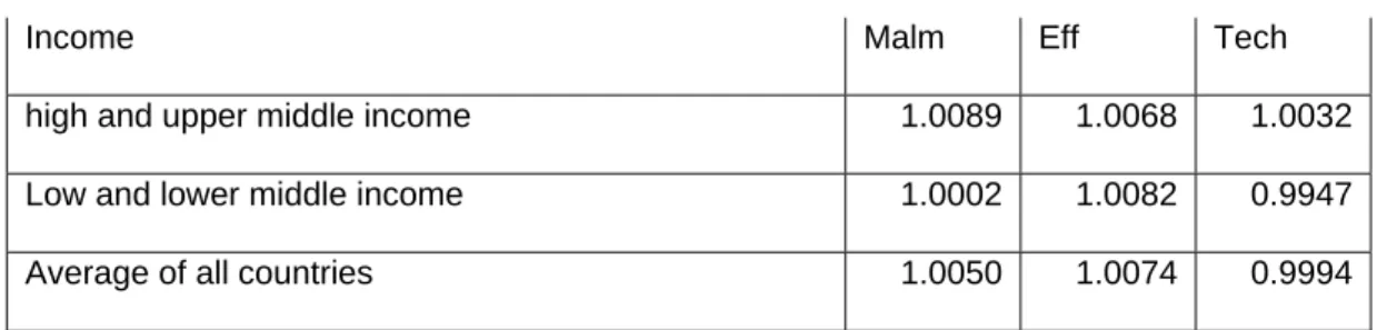
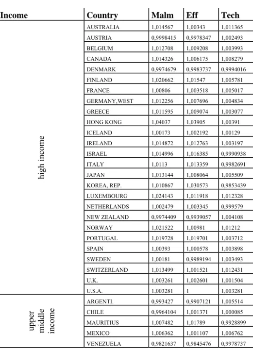
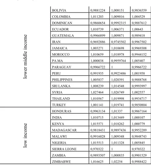
Table 1: Average Malmquist Productivity Change Index and its Components across Countries (1965-1990) ... 78 Table 2: Average Malmquist Productivity Change Index and its Components
(1965-1990) ... 79 Table 3: Fixed Effects OLS Regressions on Malmquist Productivity Change
Index ... 80 Table 4: Fixed Effects OLS Regressions on Efficiency Change Index ... 81 Table 5: Fixed Effects OLS Regressions on Technical Change Index ... 82 Table 6: Fixed Effects GMM Estimations on Malmquist Productivity Change
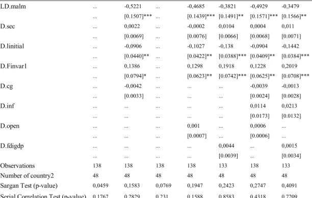
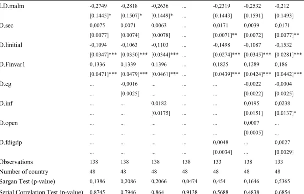
Index ... 83 Table 7: Fixed Effects GMM Estimations on Efficiency Change Index ... 84 Table 8: Fixed Effects GMM Estimations on Technical Change Index ... 85 Table 9a:Difference Estimator Results of Malmquist Productivity Change Index
(With Initial Income) ... 86 Table 9b: Difference Estimator Results of Malmquist Productivity Change Index
(Without Initial Income) ... 87 Table 10a: Difference Estimator Results of Efficiency Change Index
(With Initial Income) ... 88 Table 10b: Difference Estimator Results of Efficiency Change Index
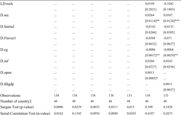
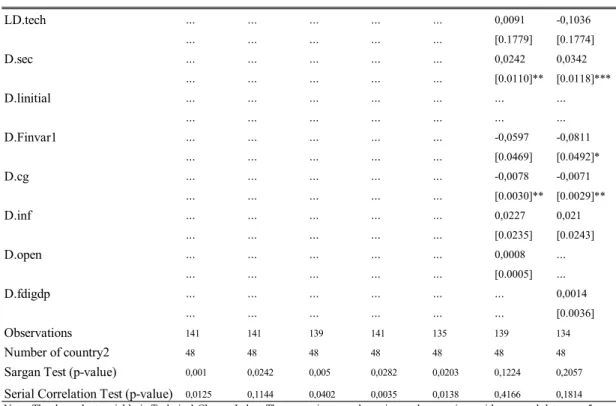
(Without Initial Income) ... 89 Table 11a: Difference Estimator Results of Technical Change Index
(With Initial Income) ... 90 Table 11b: Difference Estimator Results of Technical Change Index
(Without Initial Income) ... 91 Table 12: Summary of Static and Dynamic Productivity Change Index
Table 13: Cross Sectional Instrumental Variables Regressions on Malmquist
Productivity Change Index... 93 Table 14: Cross Sectional Instrumental Variables Regressions on Efficiency
Change Index ... 94 Table 15: Cross Sectional Instrumental Variables Regressions on Technical
Change Index ... 95 Table 16: Common Intercept Panel Data GMM Regressions on Malmquist
Productivity Change Index ... 96 Table 17: Common Intercept Panel Data GMM Regressions on Efficiency
Change Index ... 97 Table 18: Common Intercept Panel Data GMM Regressions on Technical
Change Index ... 98 Table 19a: Difference Estimator Results of Malmquist Productivity Change
Index (With Initial Income, Legal Origin) ... 99 Table 19b: Difference Estimator Results of Malmquist Productivity Change
Index (Without Initial Income, With Legal Origin) ...100 Table 20a: Difference Estimator Results of Efficiency Change Index
(With Initial Income, Legal Origin) ... 101 Table 20b: Difference Estimator Results of Efficiency Change Index
(Without Initial Income, With Legal Origin) ... 102 Table 21a: Difference Estimator Results of Technical Change Index
(With Initial Income, Legal Origin) ... 103 Table 21b: Difference Estimator Results of Technical Change Index
(Without Initial Income, With Legal Origin) ... 104 Table 22: Summary of Productivity Change Index Equations with Legal
Origin Instrument ... 105 Table 23: Robustness Check of Static and Dynamic Productivity Change
Index Equations with Lagged Values as Instruments ... 106 Table 24: Robustness Check of Productivity Change Index Equations with
LIST OF FIGURES
CHAPTER 1
INTRODUCTION
Dating as back as to 18th century there begins a huge debate on the link between financial development and economic growth. The purpose of this paper is look at the financial development growth relationship with an alternative productivity measure. We analyze the effect of financial development on Malmquist productivity index which shows the improvement of a country’s productivity relative to the world frontier.
Past literature have opposing views regarding the role of finance on growth. According to some authors, finance is one of the boosting factors for long-run growth, whereas some disagree with the stimulating effect of financial development. Many economists, such as Hamilton (1781), Bagehot (1873), Gurley and Shaw (1955), Hicks (1969), McKinnon (1974) and Schumpeter (1912), claim that financial markets spur economic growth. Hamilton (1781: 36), discusses that ‘banks were the happiest engines that ever were invented’ for stimulating growth. To illustrate, both Bagehot (1873) and Hicks (1969) emphasize that financial system enhanced England’s industrialization process by making capital mobile for ‘‘immense works’’. Besides, Gurley and Shaw (1955) stress that, in an economy where only self finance and direct finance are accessible, i.e. financial intermediaries are not involved,
economic development will be impeded as intermediaries promote the credit supply process. In addition, McKinnon (1974) claims that in less developed countries the dependence on self finance is higher. Also, he argues that liberalization will bring about easier and cheaper access to capital to entrepreneurs evolving in high quality projects that will result in economic growth and development. In addition, Schumpeter (1912) highlights the role of banks in promoting innovation. He believes that banks identify and support the enterprises that will be more successful at implementing the innovations.
On the other hand, there are some economists such as, Robinson (1952), Adams (1819) and Lucas (1988), who disagree with the supporting role of financial activity. To begin with, Robinson (1952: 86) questions the spurring effect of finance by asserting that ‘‘where enterprise leads finance follows’’. He mentions that economic growth demands its particular financial arrangements and financial system supplies. Hence, according to him growth gives rise to financial development, not the opposite. Adams (1819: 36) declares that banks harm the "morality, tranquility, and even wealth" of nations. Moreover, Lucas (1988: 6) contends that finance economic development relationship is "badly over-stressed".
In view of the papers stated above, this study investigates the link between financial development and economic growth. However, this paper differs from the existing literature in the sense that Malmquist Productivity index measures are used to measure economic performance instead of traditional measures such as per capita GDP growth or per capita capital stock growth. One of the main advantages of this index is that it can be further decomposed into two component measures, efficiency
change (diffusion) and technical change (innovation). Therefore, this technique will help us to identify the diffusion effect which McKinnon (1974) emphasized and innovation effect that Schumpeter (1912) pointed out. We calculated productivity series using data envelopment analysis and solving 4088 linear programming problems in GAMS. This is a worthwhile analysis as this methodology helps us to analyze the effects of financial development on efficiency and technical change separately and thus examine the source of productivity change. The empirical analysis is conducted on a group of countries, which includes both industrial and developing countries.
In the analysis of empirical relationship between productivity and financial development we conducted two groups of estimations:
Firstly, in addition to the fixed effects Ordinary Least Squares (OLS) estimators, the efficient Generalized Method of Moments (GMM) fixed effects estimators and GMM dynamic panel estimators is utilized to expose the relationship between the productivity and efficiency measures and the indicators of financial development. The presence of unit effects leads us to use the fixed effects model whereas the dynamic nature of the problems brings about the GMM dynamic panel estimation proposed by Arellano and Bond (1981).
Considering the unit heterogeneity effects we start with a fixed effects panel data model. We collect a panel data set of 48 countries where the data is averaged over 5-year intervals from 1965-1990. The dependent variables are Malmquist productivity index, efficiency change index and technical change index. The
explanatory variables are comprised of indicators of financial development and conditioning variables. In order to deal with endogeneity problem firstly we regress productivity measures on the lagged values of the explanatory variables as we believe that the lagged values of the explanatory variables are correlated with the regressors but not correlated with our dependent variables.
On the other hand, in the literature instrumental variables techniques are widely used to address this issue. As the explanatory variables are endogenous in most of the growth regressions, instrumental variables (IV) are used since they allow parameters to be estimated consistently. However, in the presence of heteroskedasticity the IV estimators are not only inconsistent but also inefficient (Baum and Schaffer, 2003). Although the use of heteroskedasticity consistent standard errors i.e. robust standard errors may solve the consistency problem, the efficiency problem needs to be addressed. As Baum and Schaffer (2003) points out GMM estimation brings efficiency in the presence of unknown heteroskedasticity. Therefore, we analyze the same model with fixed effects in a GMM framework where utilize the efficient Generalized Method of Moments (GMM) fixed effects estimators.
As many economic relationships are dynamic in nature, we question financial development productivity relationship in a dynamic panel data model. As Baltagi (2001) notes, there are two sources of persistence in this setup: the autocorrelation effect owing to the lagged dependent variable and the unit heterogeneity effects. In this context, we will utilize a GMM procedure proposed by Arellano and Bond (1991) in order to address the issue of omitted variables, unobserved country specific
effects and simultaneity bias. Again, the variables are averaged for five year intervals in order to get rid of business cycle effects. The empirical analysis is conducted on a panel data set of 48 countries for the period 1965-1990. We firstly, difference the regression equation to eliminate country specific effects and then we instrument the explanatory variables in the differenced equation with their lagged level values.
On the other hand, due to the simultaneity bias we instrument financial development by legal origin where we employ cross sectional GMM estimator, panel data pooled GMM estimator and GMM dynamic panel estimator. Following La Porta, Lopez-de-Silanes, Schleifer and Vishny (1998), legal origin is considered to be an appropriate instrument as it is not correlated with economic growth due to the fact that countries obtained their legal origin through colonization or occupation. On the other hand, legal origin is an appropriate instrument as it is correlated with financial development owing to the evidence that country’s legal origin affects the development of creditor rights and the enforcement of contracts in that country which is linked with financial environment or investment climate.
Besides, we utilize three econometric techniques where we instrument financial development by legal origin. Firstly, we use a cross sectional GMM estimator with a cross sectional data for 46 countries are averaged over 1965-1990. However, we believe that in this case we could not address the issue of possible endogeneity arising from the remaining right hand side variables. In addition, although the data proves the presence of unit effects as legal origin variable has no
time dimension, we estimate the model by common intercept GMM estimator. Finally, we expand our dynamic panel data model by additional legal origin instruments.
We find that there is a robust positive relationship between financial development and productivity. The dynamic models suggest that this effect comes through efficiency change channel whereas the static models suggest that this effect comes through technical change.
The plan of the paper is as follows: Chapter 2 gives a review of existing theoretical and empirical literature on finance and growth. Chapter 3 describes the calculation of Malmquist productivity index measures, and gives details of the data. Chapter 4 discusses the methodology and reports the empirical results and Chapter 5 concludes.
CHAPTER 2
LITERATURE REVIEW
It is undeniable that there is both theoretical and empirical literature that suggests a positive relationship between financial development and economic growth. Many authors even claim that financial development is a necessary condition and a good predictor for long-run economic growth.
In the Section 2.2 we will start with the theoretical literature and in Section 2.3 we will continue with summarizing the empirical literature.
2.1 Theoretical Review
In this section, we will try to explain the theoretical literature regarding the role of financial markets and institutions on economic growth. Having looked at the initial opposing views in this literature, we will firstly explain why financial markets evolved and then mention what kind of functions they serve in promoting economic growth.
Likewise many things in the history of humankind, financial intermediaries did not happen to exist instantly or without any reason. On the contrary, as Levine (1997) points out, the costs of market frictions lead to the emergence of financial markets and intermediaries. In fact, a huge literature on economic theory states that, financial instruments, markets and institutions reduce the frictions caused by information and transaction costs such as costs of acquiring information, enforcing contracts and exchanging goods and financial claims.
When considering how well the mitigating effect of financial system is working, special attention could be given to the functions that financial system provides. In Levine (1997), these functions are defined to be facilitating risk amelioration, acquiring information about investment and allocating resources, monitoring managers and exerting corporate control, mobilizing savings and easing the trading of goods, services and financial contracts.
The functions mentioned above, i.e. the ones that financial system serves; affect economic growth through two main channels which are capital accumulation and technological change (Levine, 1997). Financial system affects capital accumulation through the modification of savings rate or re-allocation of savings (Levine, 1997). On the other hand, financial system influences technological innovation through inventions and their implementations.
It is also mentioned in Gurley and Shaw (1955), Goldsmith (1969), McKinnon (1974) and Levine (1997) that across time and countries there exists no
difference between the existences of the above functions instead the difference lies in the quality of them. This quality differences will convey the relationship between finance and economic development.
In order to have a better understanding of the impact of finance on growth, one should better focus on the functions that financial intermediaries provide. One of the functions that financial markets and institutions serve is to ameliorate risks and simplify any kind of risk management, such as liquidity risk or risks associated with projects, industries, regions, etc.
Especially, financial markets provide liquidity and hence diminish the liquidity risk1. Focusing on the effect of more liquidity on economic growth there are
two aspects to be discussed. By supplying liquidity, firstly financial system can increase returns on investment and secondly can decrease the uncertainty in the economic environment (Levine, 1997).
Starting with the first aspect, one could observe that higher return projects necessitate longer term commitments of capital. However, savers are not willing to invest on long term and hence illiquid projects. At this point, financial system comes into the picture. Financial system augments liquidity of long term investments and by this way it provides funds for long term projects. As a result, it increases the demand for long term-higher return projects. Higher returns not only results in the usage of
1 Before moving to the consequences of the elimination of liquidity risk on growth, we will shortly
examine what is meant by liquidity risk and how it takes place. The instabilities inherent in the process of converting assets into a monetary tool give rise to liquidity risk. On account of the information asymmetries and transaction costs, liquidity risk arises since it is expensive to trade and there is uncertainty about the trading time and settlements. Hence, the need for liquidity brings about financial markets and institutions that provide liquidity (Levine1997).
capital its best allocation i.e. effective investment in the economy, but also attracts more investment in the economy, which will both bring in economic growth (Levine, 1997). To illustrate, Hicks (1969) claims the main engine of industrialization process was not the technological innovation as many of the products had been invented before the industrialization. He argues the important engine was the mobilization of capital markets which eased making investments. He continues that this was the case since for inventions to be made, large and long term investments were necessitated. On the other hand, as capital markets became more liquid, savers started investing on liquid assets which can easily be converted to a medium of exchange. Capital markets played a crucial role where by using short term investments of the savers they supplemented large funds for longer term projects which are illiquid. If the capital market was not that liquid this investment demand could not be fulfilled and industrial revolution will not take place. That’s why Bencivenga et al. (1966: 243) conclude that ‘‘the industrial revolution had to wait for the financial revolution…’’.
One of the financial intermediaries which lessens liquidity risk and yields higher returns on investment is stock markets where people can issue and trade securities. Stock markets help diminishing liquidity risk by assisting trade. The mechanism pursues as follows: under the umbrella of stock markets transaction costs decreases, the investments in illiquid, higher return, long term projects will rise as the individuals feel more comfortable at selling the assets whenever they want. As a result the economy will enjoy growth owing to the increase in higher return investments (Levine, 1997).
Not only stock markets but also banks may provide liquidity and bring about higher returns in investments. Bencivenga and Smith (1991), explains how banks create liquidity and mitigate its need. They enlighten the activities that banks serve which are keeping and lending deposits of many people, holding huge liquid reserves in case of any withdrawal, issuing liabilities that are more liquid then their primary assets and providing a service for self-financing of investments. Also they emphasize that “an intermediation industry permits an economy to reduce the fraction of its savings in the form of unproductive liquid assets and to prevent misallocations of invested capital due to liquidity needs” (Bencivenga and Smith, 1991: 196). In addition, Levine (1997) explains the role of banks as follows. Under normal circumstances it is impossible or too costly to observe shocks to individuals and write state-contingent insurance contracts. Instead of dealing with this complicated issue individuals may use the demand deposits or any liquid deposits offered by the banks to savers. Banks arrange these deposits to be composed of low return liquid assets and high return illiquid ones. By providing these deposits banks not only grant savers liquidity risk insurance but also increase the investments in long-run projects and hence through capital accumulation channel it boosts growth2.
Finally, before completing the effect of the elimination of liquidity risk on growth through higher returns in investment, it should be noted that higher returns may have an ambiguous effect on savings due to income and substitution effects. Other than yielding higher investment returns, financial intermediaries through reducing liquidity risk, lowers uncertainty which will in turn promote long run
2 Besides, Jacklin (1987) points out that banks will not be able to reduce liquidity risk if equity
markets are available as savers will substitute equity markets to banks. However, Gorton and Pennachi (1990) notes that this liquidity creation process will work if there are enough obstacles in the equity market.
economic growth. However, its effect on saving rates is uncertain (Levhari and Srinivasan, 1969)3. There may be a decrease in savings rates which will cause a deceleration in growth (Levine, 1997).
In addition to the liquidity risk control, financial markets and institutions such as banks, mutual funds, and security markets facilitate risk management in idiosyncratic risks. Growth may be influenced by risk diversification through capital accumulation and technological innovation (Levine, 1997).
Looking at the former, as Levine (1997) explains, the amelioration of risk may bring about an increase in high return investments. Seeing that higher return projects are more risky than lower return ones savers have an incentive for not to invest on high return projects. Obstfeld (1994), mention the role of higher risk diversification in shifting investors from low-risk lower return projects to high risk higher return ones (Saint-Paul, 1992; Devereux and Smith, 1994 and Levine, 1997). This portfolio shift may bring about capital accumulation which would end up with economic growth. However, as discussed above, the impact of higher returns on saving rates is uncertain. Higher returns may result in a decrease in saving rates leading to a fall in long-run growth.
On the other hand, amelioration of risk has growth implications through technological innovation. Since there is no guarantee for making successful innovations, or no exact timing of them or exact amount of money needed for them,
3 The confidence bred by a stable environment may lead to a decrease in savings rate due to the
relaxation of savers. Also, the savings rate may increase owing to the environment which is very suitable to make an investment.
innovations are risky. Nonetheless, a successful innovation not only brings in profits to corresponding agent that implemented it but also generates technological change. At that point, financial systems, offer diversified portfolio’s including investments in risky innovative projects. By this way, financial system helps investors to diversify risk and at the same time promote innovations which would speed up technological change, and result in economic growth (King and Levine, 1993c; Levine, 1997).
The second function that financial markets serve is acquiring information and improving the allocation of capital. As Carosso (1970) states gathering information about firms, their managers and market conditions are not an easy and costless job due to the fact that this process needs not only time but also capacity. Therefore, if there is high information costs, investors either will not be able to monitor projects or will have scarce information. As a result, investors simply won’t invest on the projects that they would with enough information. Hence, resources will not be allocated efficiently in the presence of high information costs (Levine, 1997). In fact, Greenwood and Jovanovich (1990) illustrates that financial agents can economize on the cost of gathering information. By the help of financial intermediaries, information acquisition costs fall which leads to a situation where investments are made to the projects having the highest value use, in other words savings will be allocated more efficiently (Levine, 1997).
Stock markets are one of the financial intermediaries that serve to provide information. By just looking at the published prices, the investors can acquire free information reflecting the company’s run of business. Investors won’t waste their
resources for information which will lead to a reduction in information costs. As there are limited resources, this will bring about better resource allocation and spur growth4 (Levine, 1997).
The effect of this function on growth, works through both capital accumulation and technological innovation channels. If a country’s financial system is good at selecting most promising firms and managers, there will be a more efficient resource allocation. As a result, the economy will enjoy growth through capital accumulation channel (Greenwood and Jovanovic, 1990). For instance, in mid-1800s, England’s financial system was so organized that capital was flowing to its highest value use definitely and quickly (Bagehot, 1873). England’s financial system's organization, which is good at spotting the best production technologies and sponsoring them, is the reason behind England’s greater economic development compared to the other countries at that time (Levine, 1997).
Next, financial system also leads to innovation by decreasing information acquisition costs. Together with, identifying best production technologies as mentioned, financial intermediaries identify firms that would be best at starting the production of new goods and production processes (King and Levine, 1993c; Levine, 1997). The mechanism pursue as follows. After spotting the firms which have the
4 The capacity and degree of liquidness of stock markets alters the ability of stock markets in
acquiring information about investments. Firstly, in the presence of larger stock markets, the participants will be more motivated to gather information due to the possibility of higher returns (Grossman and Stiglitz, 1980). Similarly, in the presence of the more liquid the stock markets the participants will be more motivated to gather information due to the possibility of higher returns owing to the fact that in the presence of liquid stock markets transactions can be made without facing any frictions. (Kyle, 1984; Holmstrom and Tirole, 1993). As a result, with larger and liquid stock markets resources will be allocated more efficiently, which will bring about an enhancement in growth.
best chances of successful innovations, financial intermediaries provide these firms capital or loans for investing on innovations which leads to long run growth through technological innovations.
Up to now, the information costs before the investment decisions were made, was considered. However, as Levine (1997) declares there also exist costs after financing the activity such as information acquisition and enforcement of monitoring firm managers and exerting corporate control.
As a third function, financial systems gather information, monitor managers and exert corporate control after the projects are funded (Levine, 1997). In the absence of corporate control, there would be impediments to mobilization of savings, which avoid capital flowing to its highest value use. On the other hand, with well functioning financial systems monitoring and enforcement costs will lessen. This reduction in costs will bring about reductions in obstacles in efficient investment (Thadden, 1995; Levine, 1997). Therefore, through efficient investment there will be better resource allocation.
An example for this is given in Levine (1997), which is ‘delegated monitor arrangement’ property of financial intermediaries. Suppose there is a borrower who needs funds from outside creditors. Yet, instead of all savers trying to monitor the borrower financial intermediaries monitors and lends which will decrease monitoring costs of savers (Diamond, 1984). In other words, growth comes through better resource allocation.
Now, capital accumulation channel works through the following mechanism. Financial arrangements exert corporate control that improves the allocation of capital and hence results in higher capital accumulation (Bencivenga and Smith, 1993; Khan, 1994 and Levine, 1997).
There exists no consensus on whether stock markets exert corporate control or not. Jensen and Meckling (1976) argue in the favor of stock markets and claim that stock market performance of a firm’s shares will reveal information about the success of managers. By associating stock performance to managerial administration savers will fulfill their concern about their investment’s goings-on (Verrecchia, 1982; Jensen and Murphy, 1990).
In contrast, others question whether stocks markets exert corporate control. Myers and Majluf (1984) declare that insider outsider information asymmetries may reduce the effect of stock market takeovers on promoting corporate control. As Levine (1997) also mentions, during the takeover process outsiders will be less informed comparatively. Thus, outsiders may demand a premium for the purchase of the company.
Besides Stiglitz et al. (1988) and Morck et al. (1990) disagree with the promoting role of stock markets on corporate governance (Levine, 1997). They assert that liquid stock markets worsen resource allocation due to the takeover effects. They reason their argument as follows: After the takeover, the new shareholders will relocate the capital from the stakeholders to themselves so as to gain profit. However, this new profit mechanism will hurt efficiency of resource
allocation. In addition, Shleifer and Vishny (1986) and also Bhide (1993) stresses liquid stock markets lessen the exit costs which will in turn reduce the motivation for keeping an eye on managers and firm’s on goings.
Mobilization of savings is another function of financial systems which will yield in economic growth through both capital accumulation and technological innovation channel (Levine, 1997).
By pooling distinct savers’ capital, financial systems lead to economic growth through capital accumulation channel. Firstly, by mobilization of savings financial systems solve the scale inefficiency problem (Sirri and Tufano, 1995). By pooling savings financial intermediaries can provide necessary capital to production processes which may not be able to start by individual financing due to scale inefficiency. Next, mobilization of savings brings new financial instruments. By using these instruments agents can hold diversified portfolios or more liquid assets and they can invest in efficient scale firms. To summarize, mobilization leads to better resource allocation by increasing the scale of the firms, enhancing risk diversification and providing liquid assets (Sirri and Tufano, 1995; Levine, 1997).
As a final function financial system facilitates exchange. The link between this function and growth depends on specialization. Financial intermediaries, by facilitating exchange function, reduce the cost of transactions and hence promote specialization which has a positive effect on economic development (Levine, 1997).
2.2 Empirical Literature
As mentioned in the previous section, financial development might be a very important factor in spurring growth. After having emphasized the theoretical ties in the previous section, now, we will focus on the empirical literature.
Among the body of literature in this area, we will follow an econometric approach which goes from general to specific. Therefore, we will include a wide spectrum of empirical papers with different techniques, ranging from cross section to panel data.
Cross country growth regressions aggregate economic growth over time and analyze the link between growth and financial indicators. To begin with, King and Levine (1993b) develop the cross sectional study of Goldsmith (1969) in such a way that they increase not only the cross sectional dimension but also time dimension and the number of control variables. Apart from Goldsmith’s analysis they investigate the effect of financial development on productivity and capital accumulation. Using a large cross section of 80 countries, King and Levine (1993b) analyze the relationship between financial development and growth performance from year 1960 to 1989. They examine whether the level of financial development affects current and future rates of the sources of the growth and growth. The level of financial development is measured by four indicators which are: the ratio of financial intermediary system to nominal output i.e. the ratio of liquid liabilities to GDP; the ratio of bank credit to bank credit plus central bank’s domestic assets; the ratio of credit issued to the private firms to total domestic credit and the ratio of credit issued to the private firms
to GDP. On the other hand, they use three growth indicators which are: real per capita GDP growth, real per capita capital growth and productivity growth which is measured as Solow residual5. Employing linear regression and controlling for possible determinants of growth such as initial income, educational attainment, inflation, black market exchange rate premia, government expenditure, openness to trade and political instability, King and Levine (1993b) find a strong and robust correlation between growth and channels of growth. In addition, they show that financial development predicts long run growth. However, the results do not formally imply causality.
Since we are mentioning the studies linking financial development and growth, the natural question follows as whether stock markets and/or banks lead to economic growth.
While some authors believe that especially stock market development triggered economic growth, and others stress the role of banks. On the other hand, Levine and Zervos (1998) simultaneously investigate the effects of stock markets and banking sector development on growth. In addition, they analyze whether stock markets and banks provide different services. In their study, they use a sample of 47 countries from 1976 through 1993. They examine whether measures of stock market size, stock market liquidity, volatility, integration with world capital markets and banking development influences current and future rates of growth and sources of growth. The size of stock market is evaluated by the value of listed domestic shares on domestic exchanges divided by GDP. In order to measure stock market liquidity
5 Solow residual is defined as real per capita GDP growth minus the product of production function
they used two different indicators which are stocks turnover ratio, i.e. value of trades of domestic shares on domestic exchanges divided by the value of listed domestic shares, and value traded ratio, i.e. the value of trades of domestic shares on domestic exchanges divided by the GDP. Furthermore, they use bank credit to the private sector as a share of GDP to measure banking sector progress. Besides, real per capita capital growth, productivity growth, private savings and real per capita GDP growth are used to measure sources of growth and growth. In their cross county study, in addition to the linear regression, they employ instrumental variables techniques while they control for possible determinants of growth. Levine and Zervos (1998) find a strong positive and robust correlation between current and future rates of ‘growth of output, capital accumulation and productivity’ and stock market liquidity and banking sector progress. However, they empirically find that there is no correlation between financial indicators and savings rate. Additionally, they show that banks and stock markets provide different functions in spurring growth as they jointly enter to the regressions with significant positive coefficients.
On the other hand, simultaneity bias is one of the concerns of financial development versus growth literature. As there was both evidence on finance following growth and growth being triggered by finance, there was a need for techniques taking simultaneity bias into account. One of the appropriate techniques is using an instrumental variable which is not correlated with the dependent variable, i.e. growth indicator, but highly correlated with the independent variable which leads to endogeneity, i.e. financial development indicator.
Following La Porta et al. (1998), many authors used legal origin as an instrument for financial development6. Legal origin is an appropriate instrument as it is not correlated with economic growth due to the fact that countries obtained their legal origin through colonization or occupation. On the other hand, legal origin is an appropriate instrument as it is correlated with financial development owing to the evidence that country’s legal origin affects the development of creditor rights and the enforcement of contracts in that country which is linked with financial environment or investment climate.
To start with, Levine (1999) studies not only whether legal and regulatory environment determine level of financial intermediary development but also the causality issue between financial development and growth. Firstly, he measures financial development by the indicators used in King and Levine (1993b). In addition, he uses the national legal origin measure from La Porta et al. (1998). Using dataset consisting of a cross section of 49 countries between the years 1980-1989 and applying OLS techniques between indicators of creditor rights and financial development he finds that there exists a strong relation between creditor rights and financial development. He controls for simultaneity bias by instrumenting financial development with legal origin; however, even stronger evidence is found leading the same conclusion that there is a strong relation between creditor rights and financial development. When he looks at the efficiency of legal system in enforcing contracts with the same procedure, he finds the efficiency of legal system in enforcing contracts spurs financial development. On the other hand, as the quality of
6 LaPorta et al. (1998) collect the data on legal system for 49 countries and show that legal origin—
British, French, German, or Scandinavian law—characters the laws regarding creditor rights laws and the efficiency of the enforcement of these laws in that country.
accounting standards plays a critical role in constructing financial contracts, he checks the effect of them on financial growth by using an index of comprehensiveness of company reports. Again with the same procedure, the results indicate that accounting standards positively affect financial intermediary development while this results are not that strong compared to the other legal and regulatory environment measures. In order to handle whether exogenous component of financial intermediary development triggers growth, he extends the study of King and Levine (1993b). Using the data of 45 countries from year 1960 to 1989, he instruments financial development indicators with both creditor rights, accounting and legal origin indicators while he uses Generalized Method of Moments (GMM) framework7. In addition, he controls for other factors such as initial per capita GDP, initial secondary school enrollment, the degree of ethnic diversity, government consumption to GDP, inflation rate, ratio of exports plus imports to GDP. He finds that the exogenous component of financial development leads to economic growth where the result is not driven by simultaneity bias.
Next, Levine (1998) investigates the sources of the cross country differences in banking sector development. In fact, he examines whether legal rights of creditors, the efficiency of contract enforcement and the legal origin determine the level of banking sector development in that country. Moreover, in his paper he assesses whether the exogenous component of banking sector development is linked with growth, capital stock accumulation and productivity growth. He uses data on 49 countries over the period 1976-1993, where he measures banking sector development by credit allocated by the commercial and other deposit taking banks to the private
sector divided by GDP. In order to assess creditor rights he defines a creditor index indicating the rights written in law books. In addition, he constructs an enforcement index which is the average of two indexes constructed by International Country Risk Guide (ICRG). On the other hand, he takes the legal systems’ origin measure from La Porta et al. (1998). Firstly, by using OLS with averaging the data over 1976-1993 periods, he concludes that rights of creditors and the efficiency of contract enforcement positively affects banking sector development. Also, by adding dummy variables for legal origin he finds that legal origin also explains the cross country differences in banking sector development. Next, by using GMM instrumental variable estimators and controlling for several factors, he shows that the exogenous component of banking development enhances growth, capital stock accumulation and productivity no matter it is instrumented by creditor rights, efficiency of contract enforcement or legal origin.
Next we discuss the panel data techniques. Note that one of the advantages of using panel data is the addition of time dimension. Levine et al. (2000) improve past work on finance growth literature by introducing recent panel data techniques developed by Arellano and Bond (1991) and Arellano and Bover (1995), confronting the potential biases caused by simultaneity, unobserved country specific effects and omitted variables. On the one hand, they control for unobserved specific effects, unlike cross sectional studies they are not considered as a part of the error term. On the other hand, they control for simultaneity bias in a GMM panel data framework developed by Arellano and Bond (1991) and Arellano and Bover (1995). The cross sectional studies can not always consider instruments for all of the regressors whereas the panel studies can, as they use instruments based on the past realizations
of explanatory variables (Levine, 2000). However, panel studies consider a weal type of exogeneity. Levine et al. evaluate the effect of exogenous component of financial development on economic growth and whether the differences in legal and accounting systems affects the level of financial development. They use real per capita GDP growth in order to assess economic growth and use three measures of financial intermediation which are: liquid liabilities of the financial system divided by the GDP, the ratio of commercial bank assets divided by commercial bank plus central bank assets and the value of credits by financial intermediaries to the private sector divided by GDP. They collect data on 74 countries from 1960 to 1995. They employ both panel data GMM estimators and cross sectional instrumental variable estimators. They average the panel data set over five year intervals for the GMM techniques for 74 countries whereas they average all the data such that there is one observation per country, for the cross section for 71 countries. The results show that the exogenous component of financial intermediary development triggers economic growth. Also, this paper finds that legal and accounting environment helps to explain cross country differences in financial development where the countries that put much emphasis on creditor rights, contract enforcement and accounting standards positively influence the functioning of financial system. The methodology that we used in this thesis gets the motivation from this paper.
Beck et al. (2000), investigate the link between financial intermediary development and sources of growth. They use almost the same dataset and econometric techniques with Levine et al. (2000) but they differ in the sense that in addition to economic growth they evaluate the link between finance and sources of growth which are total factor productivity (TFP), physical capital accumulation and
private savings rates. Their results suggest that better financial intermediation will bring about higher economic growth and TFP. However, taking physical capital accumulation and private savings rates into account, the paper finds no robust relationship between financial development and physical capital accumulation or private savings.
Rousseau and Wachtel (2000), empirically assess the relationship between growth and both banks and stock markets. They contribute to the literature in the sense that they analyze the effect of banking and stock market development on growth with recent panel data techniques. They use difference panel estimator to control for the potential biases caused by simultaneity, unobserved country specific effects and omitted variables. Using liquid liabilities to GDP as an indicator of banks performance and using measures of stock market size and liquidity (Measures of Levine and Zervos, 1998) with annual panel data, they find that not only banking sector but also stock market development enhances economic growth.
Beck and Levine (2002) develops Rousseau and Wachtel (2000)’s analysis while issuing the same hypothesis. They differ in two areas. While Rousseau and Wachtel (2000) uses annual data Beck and Levine (2002) takes the averages of the data for five year intervals. They improve former analysis by getting rid of business cycle effects. In addition they improve Rousseau and Wachtel (2000) in the sense that they run their regressions with more advanced GMM estimator called GMM system estimator. They use the same measures with Levine and Zervos (1998) with slight differences in deflating procedures. They use a data set of 40 countries for the
period 1976-1998 where they use real per capita GDP growth to evaluate economic growth. Both OLS and GMM techniques support the conclusion that stock markets and banks jointly and positively affect long run economic growth. In the light of studies above we will examine the relationship of financial development and economic growth where we use Fare et al. (1994)’s productivity measures.
CHAPTER 3
MALMQUIST PRODUCTIVITY CHANGE INDEX AND DATA
In this chapter we will first describe the Malmquist Productivity Index measures then we will describe our data. The objective of the paper is to address the question of economic growth and financial development from a different perspective. Traditionally, growth has been analyzed with the following variables: real per capita GDP growth, real per capita capital stock growth rate or total factor productivity. This paper examines the productivity component of growth and replaces economic growth with a specific productivity measure, Malmquist index introduced by Fare et al. (1994). The Malmquist productivity index is further decomposed into two component measures, efficiency change (diffusion) and technical change (innovation).
3.1 Measuring Productivity: Malmquist Productivity Index Approach
In this study, we use a Malmquist index approach whose idea was first originated from Malmquist (1953), then introduced by Caves et al. (1982) and further developed by Fare et al. (1994), who calculated the index by the relationship
between distance functions and Farrell efficiency measures. We calculated the index so as to analyze the productivity growth among a panel data of developed and developing countries.
The calculation of the index is done by data envelopment analysis, a non-parametric mathematical programming approach to frontier estimation, which enables us to calculate efficiencies relative to a non-parametric piecewise surface in other words frontier (Coelli, 1996). The advantages of Malmquist productivity index could be stated as follows: It neither requires price information in the calculations nor imposes a functional form. In addition, it does not assume that all decision making units are fully efficient. Finally, the main advantage of this index is that it allows for technical change and technical efficiency change decomposition.
Although there are too many definitions of productivity used in the literature, what productivity basically refers to is the relationship between the quantity of outputs of goods and services produced and the quantity of resources employed in production process (Fabricant, 1969; Kendrick, 1977). Having this simple definition in mind, we will start with a case where total factor productivity is calculated before directly moving to the explanation of Malmquist index.
Suppose there is an economy producing a single output, represented by vector y, using a single input, represented by vector x, in its production process which holds in two periods, t and t+1. So, in the first period, we have input-output mix
and in the following period we have . As total factor productivity is
) , ( t y t x ) 1 , 1 ( + + yt t x
measured by the quantity of output divided by the amount of all inputs used in production, the total factor productivity growth from year t to t+1 becomes:
t x t y t x t y TFP / 1 / 1 + + =
However, things get more complicated if we introduce many inputs and/or outputs. At this point, we need to introduce input and output distance functions which are the reciprocals of the technical efficiency measures8.
As defined in Fare et al. (1994), the production technology St is the technology set which is comprised of feasible input output vector combinations. It is
defined formally at time t as: .
⎭ ⎬ ⎫ ⎩ ⎨ ⎧ = xtcan produce yt t y t x t S ( , ):
Following Shepard (1970) or Fare (1988), Fare et al. (1994), defined the Output distance function at time t as:
{
xt yt St}
t y t x o t D ( , )=infθ:( , /θ)∈ =(sup{
θ:(xt,yt /θ)∈St}
)−1.This distance function measures the maximal proportional expansion of output vector given inputs vector in relation to the technology at time t. Note
that, if and only if . Moreover, output distance function t y xt 1 ) , ( 0 xt yt ≤ t D t S y xt, t)∈ ( 8
In Appendix A, more detailed discussion of input and output oriented productivity measures is presented.
is equal to one if and only if is on the on the best practice frontier. In terms of Farrell’s technical efficiency terminology, input output vectors , with the
property corresponds to be the technically efficient allocations. ) , (xt yt ) , (xt yt 1 ) , ( 0 xt yt = t D
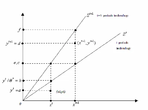
To have a better understanding, look at the Figure1. There are two different reference technologies: period t and t+1. In addition, there is only one DMU, producing a single output using a single input, is operating at at period t
and at period t+1. It can be observed that technical advance has
occurred between the year t and t+1, i.e. . In the figure, since the observed
production at t is interior to the boundary of technology at t, is not technically efficient. Given , maximum feasible production is at ( ). In other words, there is still room fro expanding output. The technical efficiency measure with respect to t t S t y t x , )∈ ( 1 ) 1 , 1 ( + ∈ + + t S t y t x 1 + ⊂ t S t S ) , (xt yt (xt,yt) t x yt/θ*
th period’s technology, which is value of the distance
function 0( , ), is Oa/Ob, which is less than 1. t t t y x D
Figure 1. The Malmquist Output-Based Index of Total Factor Productivity
On the other hand, in order to improve and introduce the Malmquist index, Fare et al (1994) defined output functions relative to different time periods. To illustrate, the output distance function at time t can be defined as:
{
xt yt St}
t y t x tD0( +1, +1)=inf θ:( +1, +1/θ)∈ . This distance function measures the maximal proportional change in outputs required to make feasible in relation to the technology at t, whereas distance function
) , (xt+1 yt+1
{
1}
1 0+ ( , )=inf :( , / )∈ + t t t t t t x y x y SD θ θ measures the maximal proportional change in
outputs required to make feasible in relation to the technology at t+1. If we again look at the figure, is no more feasible according to the reference technology at time t. Moreover, the value of distance function, at with
) , (xt yt ) , (xt+1 yt+1 ) , (xt+1 yt+1
respect to reference technology at time t is ‘Od/Oe’, which is greater than 1. Besides, the value of distance function, at with respect to reference technology at time t+1 is ‘Oa/Oc’, which is less than 1.
) , (xt yt
In order to get the intuition behind the construction of Malmquist index, following Fare and Grosskopf (2000) we will start simple where we will not use time subscripts. Also, suppose that the Decision Making Units (DMU’s) are operating under constant returns to scale (CRS) and strong disposability of inputs assumptions. Observe that, ( , ) (1,1) o D x y y x o
D = using the general ‘homogeneity of degree 1 in
y’ property of output functions and ‘homogeneity of degree -1 in x’ property which holds only in CRS assumption (Fare and Grosskopf, 2000)9.
Now, combining above observation with the total factor productivity definition, by simply substituting the input and output combinations with their time indexes, one would get:
) , ( ) 1 , 1 ( ) 1 , 1 ( / ) , ( ) 1 , 1 ( / ) 1 , 1 ( / 1 / 1 t y t x o D t y t x o D o D t y t x o D o D t y t x o D TFP t x t y t x t y + + = + + = = + + , where is
the output distance function relative to the reference technology from period t (Fare and Grosskopf, 2000). (.) o t D 9 ( ,θ )=θ (x,y),∀θ >0and o D y x o D (θ , )=(1/θ) (x,y),∀θ >0 o D y x o D
Depending on the benchmark technology period chosen, the Malmquist Productivity Index is a total factor productivity index, and it is defined to be
) , ( ) , ( ) , ( ) , ( 1 0 1 1 1 0 1 0 1 1 0 t t t t t t t t t t t t t t y x D y x D M or y x D y x D M + + + + + + + =
= if period t or period t+1 are taken to
be the reference technology respectively (Caves et al., 1982; Fare et al., 1994). In any case, a value greater than one indicates that there has been an improvement in productivity between period t and t+1 relative to the benchmark technology.
So as to avoid choosing arbitrary benchmarks, following Fischer (1922)10, Fare et al. (1994) introduced the Malmquist index to be the geometric mean of the t and t+1 Malmquist Indexes:
2 / 1 1 0 1 1 1 0 0 1 1 0 1 1 0 ) , ( ) , ( ) , ( ) , ( ) , , , ( ⎥ ⎦ ⎤ ⎢ ⎣ ⎡ = + + ++ + + + + t t t t t t t t t t t t t t t t t y x D y x D y x D y x D y x y x M .
This expression could be rewritten as (Fare et al. ,1989, Fare et al. 1992, Fare et al. 1994): 2 / 1 1 0 0 1 1 1 0 1 1 0 0 1 1 1 0 1 1 0 ) , ( ) , ( ) , ( ) , ( ) , ( ) , ( ) , , , ( ⎥ ⎦ ⎤ ⎢ ⎣ ⎡ × = + + + + ++ ++ + + + t t t t t t t t t t t t t t t t t t t t t t y x D y x D y x D y x D y x D y x D y x y x M
On the one hand, the ratio outside the brackets measures the change in relative efficiency between years t and t+1. What is meant by relative efficiency is that how the DMU performs relative to the benchmark technology with given set of
10 Fare and Grosskopf notes that they used the idea of the construction of Fischer Ideal Index. In the
sense that Fisher constructed this index by using the geometric mean of upper and lower bound of the index. In fact, Fischer ideal index is the geometric mean of Paasche index and Laspeyres index.
inputs. In other words, relative efficiency assesses how far the actual production to the benchmark production in that year is.
Efficiency change component of productivity change: ( , ) ) , ( 0 1 1 1 0 t t t t t t y x D y x D+ + +
On the other hand, the geometric mean of the two ratios inside the brackets captures the shift in technology, in other words shift in best practice frontier between the two periods evaluated at xt and xt+1. As (Fare and Grosskopf, 2000) explains
it is the geometric mean of shifts measured at xtand xt+1.
Technical change: 2 / 1 1 0 0 1 1 1 0 1 1 0 ) , ( ) , ( ) , ( ) , ( ⎥ ⎦ ⎤ ⎢ ⎣ ⎡ + + + + + + t t t t t t t t t t t t y x D y x D y x D y x D
Suppose xt =xt+1 and yt = yt+1then Malmquist productivity index is
equal to one which implies no change11. For values greater than one, efficiency change component will indicate that the country has improved its relative technical efficiency during the period considered and experienced diffusion of technology.
The above Malmquist Index and its decomposition to the efficiency change and technical change component measures can be graphically represented in Figure1 with the following distances.
11 This does not imply that Technical Change component and Efficiency change component is equal to
2 / 1 1 1 0 0 / 0 0 / 0 0 / 0 0 / 0 0 0 0 0 ) , , , ( ⎥ ⎦ ⎤ ⎢ ⎣ ⎡ ⎟ ⎠ ⎞ ⎜ ⎝ ⎛ ⎟⎟ ⎠ ⎞ ⎜⎜ ⎝ ⎛ ⎟ ⎠ ⎞ ⎜ ⎝ ⎛ ⎟⎟ ⎠ ⎞ ⎜⎜ ⎝ ⎛ = + + c a b a f d e d a b f d y x y x M t t t t 2 / 1 0 0 0 0 0 0 0 0 ⎥ ⎦ ⎤ ⎢ ⎣ ⎡ ⎟ ⎠ ⎞ ⎜ ⎝ ⎛ ⎟ ⎠ ⎞ ⎜ ⎝ ⎛ ⎟ ⎠ ⎞ ⎜ ⎝ ⎛ ⎟⎟ ⎠ ⎞ ⎜⎜ ⎝ ⎛ = b c e f a b f d
It can be seen inside the brackets of the last expression that technical change component measures the shift in frontier between two periods. It is the geometric mean of shifts from period t to t+1. The expression outside the brackets, gives the relative efficiency at t and t+1 which evaluates the actual production relative to the benchmark production. The Malmquist index, which displays the changes in the productivity, is the product of these measures. Values greater than one show improvement in the productivity index over time and values smaller than one indicate deterioration in performance. Note that, the components do not have to move in same directions, on the contrary, they could move in opposite directions. In conclusion, Fare et al. (1994) defined a productivity growth index which can be further decomposed into the product of two indexes: efficiency change and technical change. While efficiency change accounts for catching up the frontier, the technical change accounts for innovation.
In our study, we are interested in estimating productivity changes along a wide set of countries. Therefore, Malmquist productivity index is calculated by non-linear programming techniques. As we mentioned before, the index will be used to investigate the productivity growth among countries.
In our model, we assume that there are k=1,2…K countries using n=1,2…N inputs at each time period t=1,2…T in order to produce m=1,2,…M outputs
. In the model, capital and labor are assumed to be the input variables and the GDP of each country is assumed to be the output value.
t k n x , t k m y ,
The reference technology in period t is constructed as:
⎪ ⎪ ⎪ ⎭ ⎪⎪ ⎪ ⎬ ⎫ ⎪ ⎪ ⎪ ⎩ ⎪⎪ ⎪ ⎨ ⎧ = ≥ = = ≤ =
∑
∑
= = K k z N n x z M m y z y y x S t k t k n K k t k t k K k t k t m t t t ,... 1 0 ,... 1 ,... 1 : ) , ( , , 1 , , 1 ,where constant returns to scale is assumed.
The following four distance functions are calculated for each pair of years t to compute the Malmquist Productivity Index and its components.
1) , 2) , 3) , 4) . So for each
k′=1…K these four linear programming problem can be defined as:
) , ( 0 t t t x y D 1( 1, 1) 0 + + + t t t x y D ( 1, 1) 0 + + t t t x y D 1( , ) 0 t t t x y D + 1)
(
)
(
)
K k z N n x x z M m y z y to subject y x D t k t k n t k n K k t k t k m K k t k t k m k k t k t k t ,..., 1 0 ,..., 1 ,..., 1 max , , , 1 , , 1 , , 1 , , 0 = ≥ = ≤ = ≤ = ′ = = ′ ′ ′ − ′ ′∑
∑
θ θ2)
(
)
(
)
K k z N n x x z M m y z y to subject y x D t k t k n t k n K k t k t k m K k t k t k m k k t k t k t ,..., 1 0 ,..., 1 ,..., 1 max 1 , 1 , 1 , 1 1 , 1 , 1 1 , 1 , 1 1 , 1 , 1 0 = ≥ = ≤ = ≤ = + + ′ + = + + = + + ′ ′ ′ − + ′ + ′ +∑
∑
θ θ 3)(
)
(
)
K k z N n x x z M m y z y to subject y x D t k t k n t k n K k t k t k m K k t k t k m k k t k t k t ,..., 1 0 ,..., 1 ,..., 1 max , 1 , , 1 , , 1 , 1 , 1 1 , 1 , 0 = ≥ = ≤ = ≤ = + ′ = = + ′ ′ ′ − + ′ + ′∑
∑
θ θ 4)(
)
(
)
K k z N n x x z M m y z y to subject y x D t k t k n t k n K k t k t k m K k t k t k m k k t k t k t ,..., 1 0 ,..., 1 ,..., 1 max 1 , , 1 , 1 1 , 1 , 1 1 , , 1 , , 1 0 = ≥ = ≤ = ≤ = + ′ + = + + = + ′ ′ ′ − ′ ′ +∑
∑
θ θIn order to find out the Malmquist productivity index, we need to solve the above equations.